Abstract
A significant majority of overhead transmission lines’ (OHLs) outages is due to backflashovers caused by direct lightning strikes: the realistic assessment of the lightning performance is thus an important task. The paper presents the analysis of the lightning performance of an existing 150 kV Italian OHL, namely, its backflashover rate (BFOR), carried out by means of an ATP-EMTP-based Monte Carlo procedure. Among other features, the procedure makes use of a simplified pi-circuit for line towers’ grounding system, allowing a very accurate reproduction of transient behaviours at a very low computational cost. Tower grounding design modifications, aimed at improving the OHL lightning performance, are also proposed and discussed.
1. Introduction
The lightning performance assessment of high voltage (HV) and extra high voltage (EHV) overhead lines (OHLs) is paramount, as the total outage rate of such lines is mostly influenced by the backflashover rate (BFOR) and the shielding failure flashover rate (SFFOR). Assuming an effective shielding of the line, as generally guaranteed by the OHL design, SFFOR contribution to the total outage rate becomes negligible and, thus, BFOR becomes largely prevalent. Because of the random nature of many parameters involved in the backflashover phenomenon, such as the ones related to lightning current waveform (polarity, current peak, front time, and time-to-half value) and line insulation (critical electric field), the BFOR should be assessed, in principle, by means of statistical and nondeterministic procedures employing the Monte Carlo method.
As the tower grounding system plays a key role for the occurrence of backflashover, an efficient Monte Carlo procedure for BFOR evaluation should employ an accurate model of tower grounding system, able to simulate the response of the system during fast transients related to lightning. Moreover, nonlinear phenomena due to soil ionisation, as well as to frequency dependence of soil parameters (soil resistivity and permittivity), should be taken into account for a realistic BFOR evaluation. Many grounding systems models are available in literature, among them, circuit-based, field-based and hybrid (using both circuit and field approaches) models are the most numerous; an exhaustive and accurate review is not possible in this paper, only a brief description is provided focusing on advantages and drawbacks of each approach. Circuit models, such as the ones described in [1,2,3,4], are simple to implement and less time-consuming; moreover, they allow the simulation of soil ionisation and can be easily coupled with electromagnetic transient programs. On the other hand, they are less accurate and do not allow including the frequency dependence of soil parameters. Field models, like the ones reported in [5,6], are the most accurate, as Maxwell’s equations are directly solved without simplifying assumptions, and allow the simulation of frequency dependence of soil parameters; on the other hand, they are computationally expensive and do not include soil ionisation representation. Hybrid models [7,8,9] combine both advantages and drawbacks of both circuit and field approaches. Last, only in recent papers, such as in [10], a time domain formulation of frequency dependence of soil parameters is given: this will also allow incorporating soil ionisation for most accurate grounding system models.
Regardless of the specific grounding system model implemented, the main drawback is that the BFOR evaluation by a Monte Carlo approach requires a massive number of simulations; for this reason, the use of a complete grounding system model is not suited, even in the case of circuit models, due to the computational effort required. Therefore, simplified procedures eschewing Monte Carlo approach were developed, most notably those suggested by CIGRE [11] and IEEE [12,13] or the ones proposed in [14,15]. On the other hand, very simplified Monte Carlo procedures were proposed in the literature [16,17,18,19,20]. The introduction of a simplified yet accurate pi-circuit model for the tower grounding system [9,21,22,23,24] drastically reduced computation times, thus allowing the use of a detailed ATP-EMTP [25] model as the simulation engine in a Monte Carlo procedure for line BFOR evaluation [26,27,28]. In the case of concentrated grounding systems, the results were also validated by comparison with the well-known CIGRE method [27].
If the line’s prospective BFOR value has to be lowered in order to bring the total line outage rate below a tolerable threshold, an essential issue is the selection of the appropriate design measures to improve the lightning performance of the OHL. The choice must obviously be performed from a technical/economic point of view, taking into account both the expected decrease in the BFOR and the cost of implementation. Some of the commonly adopted design measures to reduce BFOR are as follows.
- Reducing the tower surge impedance (in order to mitigate the stress on the insulator strings) by using guyed towers.
- Adding one (or more) shield wire(s).
- Increasing the critical flashover voltage of the line by installing longer insulator strings.
- Improving the grounding system efficiency by reducing the grounding impedance in the frequency range of interest (up to 1 MHz).
- Installing line surge arresters (on all phases or only on one phase, in all towers or only in selected towers).
The paper deals with the lightning performance evaluation of a typical Italian OHL configuration, namely a 150 kV—50 Hz subtransmission OHL operated by Terna, the Italian transmission system operator (TSO). The line is studied by means of the ATP-EMTP Monte Carlo procedure described in [26,27]; grounding system arrangements actually used by Terna are simulated by means of the pi-circuit model presented in [24], for different soil resistivities, ρg, ranging from 10 up to 2000 Ω·m. Possible countermeasures aimed at improving lightning performance are proposed and their effectiveness is evaluated by calculating the related BFOR reduction.
Section 2 of this paper describes the main features of the Italian 150 kV—50 Hz OHLs (towers, conductors, line insulation and grounding systems); Section 3 summarises the ATP-EMTP Monte Carlo procedure used to calculate BFOR, with a particular focus on the pi-circuit model of the grounding system embedded in the procedure. Section 4 reports data on the lightning performance of Terna subtransmission lines currently in operation, as well as presents and evaluates the possible design variants that can be adopted to reduce the line BFOR.
2. Main Characteristics of Terna 150 kV OHLs
2.1. Subtransmission Lines
Standard Italian 150 kV—50 Hz subtransmission lines are three-phase, single-circuit lines. Each phase is equipped with single 31.5 mm ACSR conductors, with an 11.4 m sag. There is only one shield wire, consisting in an 11.5 mm steel conductor (9.7 m sag) solidly connected to each tower peak. The average span length is 400 m [29].
2.2. Towers
The most commonly used towers in Italian subtransmission lines are steel lattice suspension towers, whose outline is shown in Figure 1a. The overall height is 31.1 m, whereas the tower base is a square with each side 4.8 m long. The coordinates of phase conductors and shield wire are instead reported in Table 1. The tower surge impedance, Zs, is ~168 Ω and has been estimated by using the following equation [30],
where h is the tower height and r is the radius at the base of the tower. Equation (1) is found by performing a conical approximation of the tower: this allows to obtain a constant tower surge impedance value, i.e., not dependent on the current waveform injected, which is very convenient to employ in statistical procedures using a very large number of lightning current waveforms, each with different parameters. In principle, the tower surge impedance value not only depends on the injected current waveform, but also on the soil resistivity value and the v(t)/i(t) response of the tower grounding system, as reported in [31]. The authors of [31] show that tower surge impedance slightly decreases with the increase in soil resistivity, as well as slightly varies with the grounding arrangement, so that Equation (1) slightly overestimates the tower surge impedance. As higher tower surge impedance values cause higher stress on line insulation, this implies that using Equation (1) causes a slight (but conservative) overestimation of the OHL BFOR value.
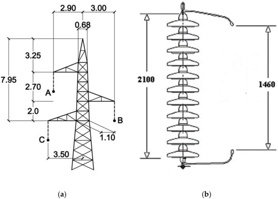
Figure 1.
(a) 150 kV overhead transmission line (OHL) tower outline (dimensions are expressed in meters). (b) Line insulation (dimensions are expressed in millimetres).

Table 1.
Phase and shield wire conductor coordinates.
Line insulation is dictated by the arching horn gap length, which in standard configurations is 1.46 m, corresponding to an 820 kV standard critical flashover voltage (see Figure 1b) [29]. The possibility to add up to four insulators in the standard insulator string, without modifying the mechanical design of the OHL, is foreseen in case the line is installed in areas with high environmental pollution.
2.3. Grounding System Arrangements
The type of tower grounding systems installed in Italian subtransmission lines is dictated by Terna unified design document LF 91 [32]: six different grounding system arrangements are available, as shown in Figure 2. Each arrangement is made of strap iron (FE 360 B, 15.887 mm radius, ρ = 0.1 × 10⁻⁶ Ω·m) buried at ~0.8 m depth; branch terminals (not shown in Figure 2) are 1.4 m long with a 45° slope (only MT1 arrangement has no branch terminal). Terna unified design prescribes the installation of each arrangement in a specific range of soil resistivity values, as shown in Table 2. Soil is considered uniform and not layered.
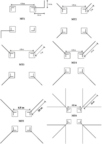
Figure 2.
Grounding systems installed in Italian 150 kV OHLs according to Terna unified design.
Table 2.
Soil resistivity range for each grounding arrangement according to Terna unified design.
3. ATP-EMTP Monte Carlo Procedure for BFOR Calculation
The BFOR is assessed by a procedure combining a Monte Carlo approach and electromagnetic transient simulations by means of ATP-EMTP. At first, Ntot lightnings (consisting of negative first strokes, positive first strokes and negative subsequent strokes) are statistically generated; NL direct strokes to the line out of the Ntot lightnings are selected by applying the Ericksson electrogeometric model [33]. Each direct stroke (assumed to be a direct stroke to the tower peak) is simulated with an ATP-EMTP complete model of the system (including OHL model, line insulation model, lightning stroke model and grounding system model) in order to check the occurrence of backflashover. The procedure stops either when a convergence tolerance criterion is fulfilled (the relative mismatch between two consecutive values of the ratio NBFO/N is lower than a fixed threshold) or when all generated lightning strokes are simulated. Finally, the BFOR of the line (faults/100 km/year) may be calculated as
where NBFO is the total number of simulated backflashovers, Nconv is the number of the generated lightning that corresponds to the convergence of the procedure and Ng is the ground flash density (flashes/km2/year). The numerical coefficient 0.6 is used, as suggested in [34], to take into account also lightning strokes within the span, which are assumed not causing backflashover. A flowchart describing the Monte Carlo procedure is reported in Figure 3. In the following subsections, a short description of the statistical input of the procedure, as well as of the ATP-EMTP sub-models of the complete system, is given.
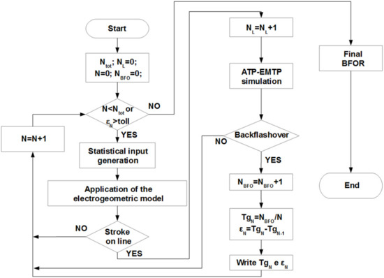
Figure 3.
Flowchart of the Monte Carlo procedure.
3.1. Statistical Inputs of the Procedure
Statistical variables are generated by the procedure:
- First and subsequent stroke lightning parameters (i.e., polarity; peak current, IP; time-to-front, tF; time-to-half value, tH)
- Line insulation (critical electric field, E0)
- Location of lightning
- Phase angle of the power frequency voltages
A detailed description of statistical distributions is given in [26,27,28,35] but is not reported in this paper for the sake of brevity. However, differently than in [26,27,28,35], the IP distribution of negative first strokes used in the presented simulations is the log-normal distribution proposed in [11] and summarised in Table 3.
Table 3.
Statistical distribution of the first negative return stroke peak current.
3.2. OHL Model
A 10 km long, 150 kV OHL is considered. Line spans are 400 m long, each simulated in ATP-EMTP by means of the J-Marty model centred at 100 kHz. At both ends, the line is connected to the surge impedance matrix and terminated on a three-phase 150 kV—50 Hz voltage system, whereas the shield wire is solidly grounded. Segments and cross-arms of the towers are modelled as lossless single-phase transmission lines with the Bergeron model, considering a Zs as evaluated with (1) and propagation speed equal to 2.99 × 10⁸ × m × s−1.
3.3. Line Insulation Model
Phase insulation is simulated by the CIGRE leader progression model [11], implemented in ATP-EMTP by means of “MODELS” language:
In Equation (3), l(t) is the leader length in meters, u(t) is the voltage across insulator in kilovolts, dG the arching horn gap length (equal to 1.46 m in Italian 150 kV OHLs) and k is the speed parameter, equal to 1.2 × 10⁻⁶ × m2 × kV−2 × s−1 and 1.3 × 10⁻⁶ × m2 × kV−2 × s−1 for positive and negative flashes, respectively. E0 is the critical electric field (kV/m), which is a statistical input of the procedure, as reported in Section 3.1.
3.4. Lightning Stroke Model
Lightning strokes are simulated by means of the well-known “Heidler” function [36], implemented in ATP-EMTP by means of “MODELS” language. The lightning waveform is given by the following expression,
In Equation (4), η is a factor adjusting the peak current value; ks is the ratio t/τ1, being τ1 and τ2 two time constants depending on tF and tH; and n is another numerical factor influencing the rate of rise of the lightning current (in all simulations reported in this paper, n has been taken equal to 5).
3.5. Grounding System Model
The grounding system of each tower is simulated in ATP-EMTP by means of the simplified pi-circuit model presented in [24] and depicted in Figure 4. The model is obtained synthesizing the full circuit model described in [4] by means of a micro-genetic algorithm optimisation procedure. The pi-circuit is able to simulate a grounding arrangement in a given soil resistivity range and also takes into account soil ionisation.
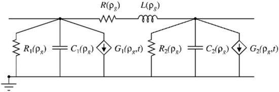
Figure 4.
Pi-circuit model.
Linear parameters R1(ρg), R2(ρg), R(ρg), L(ρg), C1(ρg) and C2(ρg) reproduce the non-ionised behaviour of the grounding system in the frequency range of interest, which has been set as 1 Hz–1 MHz.
Soil ionisation is instead reproduced by means of the two voltage controlled current generators G1(ρg,t) and G2(ρg,t), whose formulation is
In Equation (5), VRi(t) is the voltage across the resistor Ri(ρg) and the “transient resistance” Fi(ρg,t) is expressed as
where αi(ρg) and βi(ρg), respectively, expressed in Ω and in A−1, are numerical coefficients representing soil ionisation; Fi(ρg,t) is limited in the range 10−4—Ri. As in the case of pi-circuit linear parameters, αi(ρg) and βi(ρg) are also expressed as a function of ρg. Equation (6) approximates the ground resistance of a cylindrical electrode whose external radius increases when the current injected to ground increases due to soil ionisation.
3.5.1. Pi-Circuit Synthesis Procedure
The synthesis procedure yielding pi-circuit parameters is an optimisation procedure based on micro-genetic algorithm (µGA) [37], well suited to solve multi-objective and nonlinear optimisation problems. The synthesis procedure may be summarised as in the following.
- Geometrical and physical parameters of the grounding system are provided; the discretisation step of the range of soil resistivity values of each grounding system (see Table 2) is chosen.
- Pi-circuit linear parameters are calculated in frequency domain.
- Pi-circuit nonlinear parameters are calculated in time domain.
- Points 2 and 3 are repeated for each soil resistivity discretisation step.
- For each pi-circuit parameter, both linear and nonlinear, a polynomial approximation as a function of ρg (applicable in the soil resistivity utilisation range of the grounding system) is performed.
At point 1, input data of the grounding system are read, in order to create the ATP-EMTP file simulating the grounding system by means of the full circuit model described in [4]. Moreover, for each specific grounding system, the soil resistivity discretisation step is chosen: such step is 100 Ω·m for MT2, MT3, MT4, MT5, and MT6, whereas for MT1, two ρg values, 10 Ω·m and 50 Ω·m, are selected.
At point 2, for a given ρg value, pi-circuit linear parameters are calculated in the frequency domain. In the 1 Hz to 1 MHz frequency range, the input impedance of the grounding system simulated with the full circuit model, Zfull,lin(f), is calculated by performing in ATP-EMTP a frequency scan for Nf frequency values in the frequency range. In point 2, the nonlinear part of the full circuit model, which simulates soil ionisation, is not represented. The µGA optimisation procedure calculates the linear parameter set of the pi-circuit minimising the objective function
being Zpi,lin(f) the input impedance of the grounding system simulated by the simplified pi-circuit model. The optimisation procedure stops when the linear parameter set of the pi-circuit minimising Equation (7) is not updated after 1000 iterations.
At point 3, for a given ρg value, pi-circuit nonlinear parameters, i.e., α1, α2, β1 and β 2 of generators G1(t) and G2(t), are calculated in the time domain. In ATP-EMTP, a certain number Nlc of time domain simulations are executed by injecting Nlc lightning currents (with different IP, tF and tH values) in the full circuit model (in this case including soil ionisation representation), thus obtaining Nlc time plots of the ground potential rise (GPR) of the grounding system, GPRfull. Such plots are compared with GPRpi plots obtained by injecting the same lightning currents in the pi-circuit model, using in this step for the pi-circuit the linear parameters calculated at point 2. Chosen n time values t, the µGA optimisation procedure finds the optimal solutions for α1, α2, β1 and β2 minimising the objective function
for each one of the Nlc lightning currents. An Nlc-dimensional Pareto front of non-dominated optimal solutions is obtained, among which the set of α1, α2, β1 and β2 values with the minimum standard deviation is chosen.
Points 2 and 3 are then repeated for each one of the ρg values in the range of interest for the grounding system, thus obtaining an array of pi-circuit parameter values at the end of point 4.
At point 5, for each one of the arrays obtained at point 4 and each one of the pi-circuit parameters, a polynomial approximation as a function of ρg is performed. Polynomial regression is applied, starting from simple linear regression, with the aim of minimising the standard deviation between the outputs provided by the pi-circuits in Equation (8) and the ones obtained by the pi-circuits with parameters calculated by the polynomial approximations.
3.5.2. Pi-Circuit Parameters of Terna Grounding System Arrangement
All pi-circuit linear and nonlinear parameters are expressed as a function of soil resistivity ρg: for a given grounding arrangement ρg may vary in the range reported in Table 2 in Section 2.3 (with the exception of MT1 grounding arrangement: in this case, soil resistivity range is 10 to 50 Ω m). Table 4, Table 5, Table 6, Table 7, Table 8 and Table 9 report the expressions of linear parameters for the Terna grounding arrangements: in all these cases, all linear parameters are linear functions of ρg. Table 10, Table 11, Table 12, Table 13, Table 14 and Table 15 report nonlinear parameters expressions for the Terna grounding arrangements: for the MT6 arrangement, parameter α1 is approximated by a parabola, whereas in all other cases nonlinear parameters are either linear functions of ρg or constants.
Table 4.
Linear parameters for MT1 pi-circuit as a function of soil resistivity.
Table 5.
Linear parameters for MT2 pi-circuit as a function of soil resistivity.
Table 6.
Linear parameters for MT3 pi-circuit as a function of soil resistivity.
Table 7.
Linear parameters for MT4 pi-circuit as a function of soil resistivity.
Table 8.
Linear parameters for MT5 pi-circuit as a function of soil resistivity.
Table 9.
Linear parameters for MT6 pi-circuit as a function of soil resistivity.
Table 10.
Nonlinear parameters for MT1 pi-circuit as a function of soil resistivity.
Table 11.
Nonlinear parameters for MT2 pi-circuit as a function of soil resistivity.
Table 12.
Nonlinear parameters for MT3 pi-circuit as a function of soil resistivity.
Table 13.
Nonlinear parameters for MT4 pi-circuit as a function of soil resistivity.
Table 14.
Nonlinear parameters for MT5 pi-circuit as a function of soil resistivity.
Table 15.
Nonlinear parameters for MT6 pi-circuit as a function of soil resistivity.
In order to show the performances of the pi-circuit, comparisons between the pi-circuit and full circuit model are shown for two out of six grounding arrangements, namely, MT4 and MT6. Figure 5 and Figure 6 compare frequency scans of the MT4 and MT6 impedance in the 100 to 106 Hz range obtained the two, non-ionised, models. A very good agreement is found in case of MT4 arrangement in the whole range of frequencies, whereas in case of MT6, discrepancies occur starting from some thousands of kilohertz. Such discrepancies are due to the difficulty for a single pi-circuit to reproduce exactly the resonant behaviour which may occur for large grounding system arrangements at so high frequency values. These discrepancies, however, are not expected to compromise the time domain response of the pi-circuit when lightning current waveforms are injected for two main reasons: their frequency content at so high frequencies is not predominant with respect to other frequencies over the considered 1 Hz to 1 MHz range, and the effect of soil ionisation tends to accentuate the resistive behaviour of the grounding system.
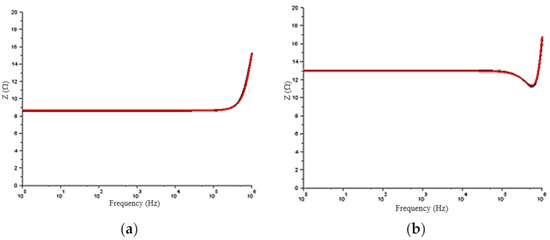
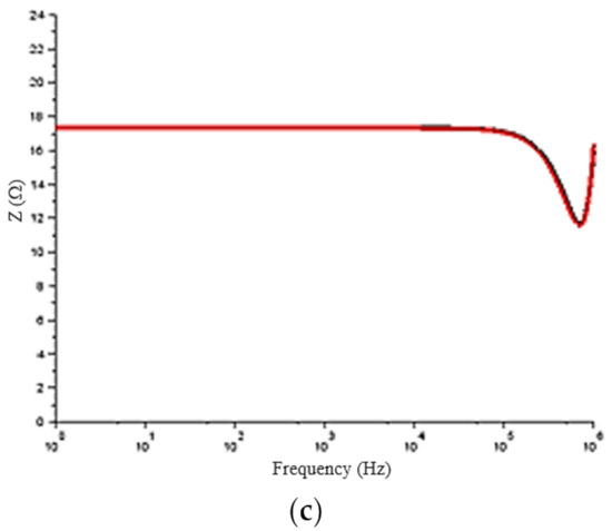
Figure 5.
Input impedance of MT4 grounding arrangement in 1 Hz to 1 MHz frequency range. Red line: full circuit model; black line: pi-circuit model. (a) ρg = 300 Ω m; (b) ρg = 450 Ω m; (c) ρg = 600 Ω m.
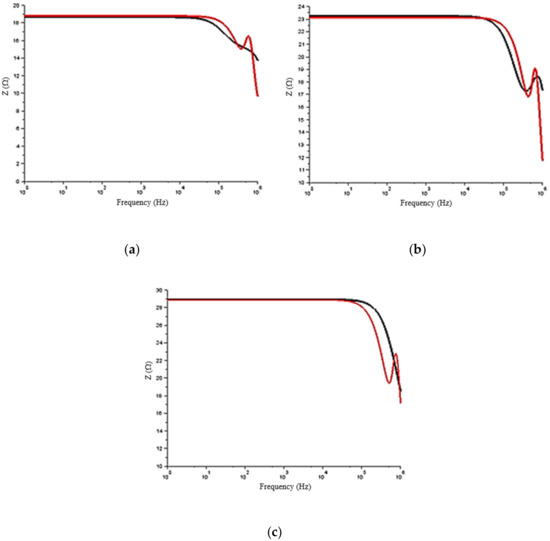
Figure 6.
Input impedance of MT6 grounding arrangement in 1 Hz to 1 MHz frequency range. Red line: full circuit model; black line: pi-circuit model. (a) ρg = 1300 Ω·m; (b) ρg = 1600 Ω m; (c) ρg = 2000 Ω m.
Figure 7 and Figure 8 compare MT4 and MT6 GPR obtained by the two ionised models: in these two simulations, the lightning current is directly injected into the grounding arrangement. Moreover, in this case, a very good agreement is found for MT4, with the largest mismatch of ~2%; most notably, even in the case of MT6, a good agreement is found, despite the discrepancies at high frequencies found in the frequency scan, with the largest mismatch of ~3% in correspondence of the front of the lightning wave in Figure 8b.
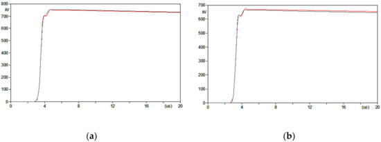
Figure 7.
GPR plots against time for MT4 grounding arrangement directly injected by a lightning current. Red line: full circuit model; black line: pi-circuit model. (a) ρg = 600 Ω m, IP = 58 kA, tF = 1.63 μs, tH = 300 μs; (b) ρg = 600 Ω m, IP = 51 kA, tF = 1.49 μs, tH = 300 μs.
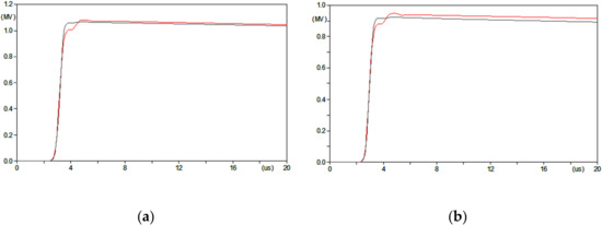
Figure 8.
GPR plots against time for MT6 grounding arrangement directly injected by a lightning current. Red line: full circuit model; black line: pi-circuit model. (a) ρg = 2000 Ω m, IP = 44 kA, tF = 1.36 μs, tH = 300 μs; (b) ρg = 2000 Ω m, IP = 38 kA, tF = 1.25 μs, tH = 300 μs.
Last, Figure 9 and Figure 10 compare the voltage across insulator (for each simulation only the voltage of the most stressed phase is plotted) due to direct strokes to tower peak obtained by the two models when the complete system is simulated with ATP-EMTP. For both MT4 and MT6, in case both of insulation withstands (Figure 9a and Figure 10a) and of backflashover (Figure 9b and Figure 10b), a very good agreement is evidenced between the two models, also with respect to the time the backflashover occurs.
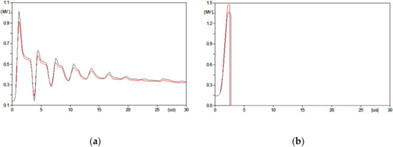
Figure 9.
Voltage across insulator (most stressed phase) against time when a 150 kV OHL equipped with MT4 grounding arrangement is struck by lightning. Red line: full circuit model; black line: pi-circuit model. (a) ρg = 600 Ω·m, IP = 39 kA, tF = 1.26 μs, tH = 300 μs; (b) ρg = 600 Ω m, IP = 99 kA, tF = 2.44 μs, tH = 300 μs.
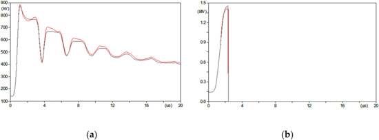
Figure 10.
Voltage across insulator (most stressed phase) against time when a 150 kV OHL equipped with MT6 grounding arrangement is struck by lightning. Red line: full circuit model; black line: pi-circuit model. (a) ρg = 2000 Ω·m, IP = 35 kA, tF = 1.19 μs, tH = 300 μs; (b) ρg = 2000 Ω·m, IP = 75 kA, tF = 1.96 μs, tH = 300 μs.
4. Results
Grounding resistance at power frequency, R50Hz, is reported in Figure 11 as a function of soil resistivity. Discontinuities are clearly due to the use of different grounding arrangements in different soil resistivity ranges, as detailed in Table 2. R50Hz values span from approximately 1.6 Ω to 29 Ω: in general, the trend of R50Hz values exhibits a less than linear increase with soil resistivity.
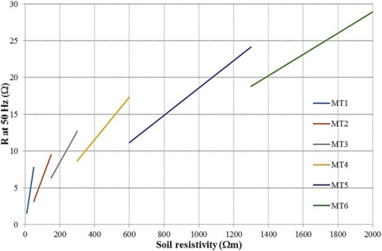
Figure 11.
Calculated values of the grounding resistance at power frequency.
Regarding the lightning performance in terms of BFOR, Ntot = 720,325 flashes, corresponding to 2,153,833 strokes (including both first and subsequent strokes), are generated. NL = 200,000 are the flashes impinging the OHL. Peak current probability distributions of Ntot and NL flashes are shown in Figure 12a,b, respectively. The plot in Figure 12a is not a perfect log-normal distribution, as it is the superimposition of three different log-normal distribution (one for negative first strokes, one for positive first strokes and one for negative subsequent strokes); peak current distribution in Figure 12b is instead obtained by applying the Ericksson electrogeometric model to the distribution in Figure 12a.
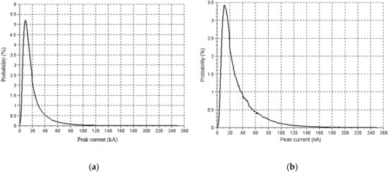
Figure 12.
(a) Probability distribution of the peak currents of the generated Ntot flashes; (b) Probability distribution of lightning peak currents impinging the OHL, in percent of the generated flashes.
Figure 13 reports the peak current probability distribution of the flashes causing BFOR of the 150 kV OHL when equipped with each of the grounding system arrangements and considering for each arrangement the highest ρg value in the range. The appearance of the band of critical peak current values in the left of the distributions in Figure 13a,e is due to subsequent strokes, which also cause the reduction of the minimum peak current value causing backflashover (this effect is instead recognisable for all distributions).
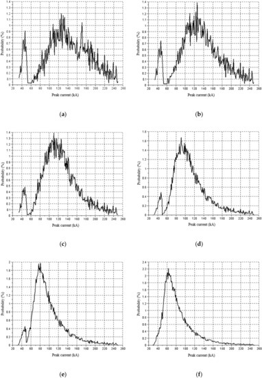
Figure 13.
Probability distribution of the peak currents of NBFO flashes causing backflashover. (a) MT1 grounding arrangement, ρg= 50 Ω m; (b) MT2 grounding arrangement, ρg= 150 Ω m; (c) MT3 grounding arrangement, ρg= 300 Ω m; (d) MT4 grounding arrangement, ρg= 600 Ω m; (e) MT5 grounding arrangement, ρg= 1300 Ω m; (f) MT6 grounding arrangement, ρg= 2000 Ω m.
Moreover, the BFOR trends of the 150 kV OHL, when equipped with each one of the grounding system arrangements and considering for each arrangement the highest ρg value in the range, are shown in Figure 14. In all cases reported in Figure 14, the Monte Carlo procedure has been stopped when all generated lightning strokes are simulated and not according to the convergence criterion described in Section 3, with the aim to show the stability (in terms of convergence) of the procedure.
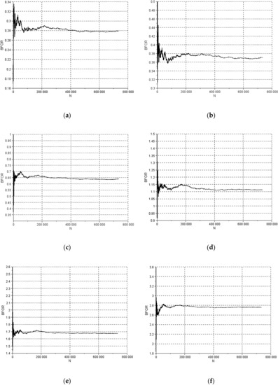
Figure 14.
Backflashover rate (BFOR) trend as a function of the generated flashes, evaluated with (2) considering Ng = 1. (a) MT1 grounding arrangement, ρg = 50 Ω m; (b) MT2 grounding arrangement, ρg = 150 Ω·m; (c) MT3 grounding arrangement, ρg = 300 Ω m; (d) MT4 grounding arrangement, ρg = 600 Ω m; (e) MT5 grounding arrangement, ρg = 1300 Ω m; (f) MT6 grounding arrangement, ρg= 2000 Ω·m.
Lastly, Table 16 summarises 150 kV OHL BFOR results, normalised for Ng = 1 ground flash density value; for each grounding arrangement both the minimum and the maximum allowable soil resistivity values have been considered, with the exception of MT1 (in this case, only the maximum soil resistivity value has been considered). Results show a tenfold increase of BFOR over the 50–2000 Ω·m soil resistivity range.
Table 16.
BFOR calculated by the Monte Carlo procedure for the simulated grounding system arrangements.
Considering that the ground flash density in a significantly large portion of the Italian territory is 4 flashes/km2/year [38], the authors examined the feasibility of countermeasures aimed at improving the OHL lightning performance.
- Given a soil resistivity range, install the first subsequent grounding arrangement.
- Change the tower design from a single to a double shield wire arrangement.
- Add additional vertical rods to the existing grounding system design.
- Install guy wires in order to reduce the tower surge impedance, as well as a ground ring to connect guy wires.
- Increase clearances and insulator string length.
The installation of line surge arresters is not evaluated in this paper, despite such countermeasure may be very effective in BFOR reduction. However, improvements in OHL lightning performance due to surge arrester installation are discussed in the literature, in [39,40], the best placement of surge arresters is treated, whereas in [41], a Monte Carlo-based procedure able to assess the flashover rate of OHLs is developed; moreover, the authors of [42] study the probability of surge arrester failures due to lightning flashes. Last, the authors of [28] apply a Monte Carlo procedure to estimate BFOR reduction due to surge arrester installation (in one or in all three phases) for a 150 kV overhead line with a very high BFOR.
In the following subsections, each one of the five above listed countermeasures is examined in detail. All presented results are normalised for the ground flash density value Ng = 1 flashes/km2/year.
4.1. Adopt a Larger Grounding System
For a given soil resistivity range, one simple approach is to adopt the first larger grounding system arrangement among the ones foreseen in Terna unified design. Obviously, this approach is only applicable up to 1300 Ω·m soil resistivity value. The solution can be straightforwardly applied for new OHLs, whereas it is not a viable option for existing OHLs, due to right of way constraints and authorization problems. The effectiveness of this solution is presented in Table 17, in terms of reductions both of R50Hz and BFOR values. The average expected BFOR reduction is ~29%, whereas the maximum expected reduction is obtained if MT4 grounding arrangement is replaced by the MT5 one (~36.5%); moreover, replacing MT5 with MT6 leads to a reduction larger than 30%.
Table 17.
Countermeasure 1: improvement of the lightning performance for different soil resistivity values.
4.2. Add a Second Shield Wire
The addition of a second shield wire allows for a reduction in the current injected into the grounding system, at a reduced expense in terms of tower weight and cost. For this countermeasure, the use of a twin-bundled shield wire instead of the single shield wire normally used by Terna has been considered: in such a way, the number of flashes striking the tower with respect to the normal design does not increase. As for countermeasure 1, this solution is only viable for new OHLs. However, its effectiveness is significantly higher if compared to countermeasure 1, as reported in Table 18; moreover, differently than countermeasure 1, it is applicable also in the highest soil resistivity range, which is the most critical in terms of BFOR. The analysis has been carried out only on the harshest soil resistivity scenarios: an average BFOR reduction of 45.6 % is expected.
Table 18.
Countermeasure 2: improvement of the lightning performance for different soil resistivity values.
4.3. Add Four Vertical Rods at the Tower Base
This countermeasure entails the installation of four vertical rods (each one 6 m long) at the tower base. Differently from the previous countermeasures, this one is applicable also for existing OHLs, as it does not increase the right of way; the expected cost is limited to few thousands euros (except in rocky soils). Clearly, the addition of the four vertical rods modifies the geometry of the grounding arrangement, so the pi-circuit synthesis procedure described in Section 3.5.1 must be reapplied; pi-circuits parameters obtained for this countermeasure are not reported in the paper. The analysis has been carried out considering the MT4, MT5 and MT6 arrangements: results obtained in terms of lightning performance evaluation (reported in Table 19) are not so good, showing a limited effectiveness of this countermeasure. Only for MT4 there is an appreciable R50Hz and BFOR reduction of approximately 10% and 14%, respectively; in case of MT6, the enhancement with respect to the currently adopted Terna practice is practically null, because of the very small contribution of the four vertical rods in reducing the v(t)/i(t) ratio of the grounding system in soils with so high resistivity values.
Table 19.
Countermeasure 3: improvement of the lightning performance for different soil resistivity values.
4.4. Install Guy Wires and Ground Ring
This countermeasure aims at reducing both the tower surge impedance (by installing four guy wires) and the grounding impedance at high frequency (by adding a ground ring to the existing grounding system arrangement). The analysis has been carried out considering only MT4 and MT5 arrangements with the additional ground ring, as shown in Figure 15. In this context, the guy wires do not fulfil any structural requirement; they are connected between the tower (~2 m below the lowest phase) and the four edges of the grounding ring. Guy wires are made of 11.5 mm aluminium clad steel ropes; self-inductances of each guy wire have been estimated using the formulation reported in [11], yielding 42 µH and 57 µH for MT4 and MT5 arrangements, respectively. Moreover, in this case, as for the previous countermeasure, the pi-circuit synthesis procedure must be reapplied since both the geometry and the lightning current injection points of the grounding arrangements are different than the standardized ones. Lightning performances are reported in Table 20. Results evidence how this countermeasure is the most effective in terms of BFOR reduction even if, differently than countermeasure 2, such reductions strongly vary depending on the guy wire length, which in turn is determined by the grounding system layout. In fact, despite a practically equal reduction of the R50Hz values for MT4 and MT5 arrangements, a higher BFOR reduction is evaluated for MT4, due to a lower inductance of guy wires.
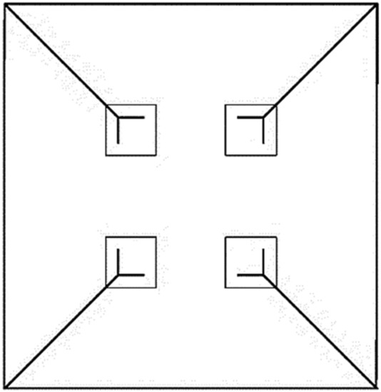
Figure 15.
MT4 and MT5 layout with ground ring.
Table 20.
Countermeasure 4: improvement of the lightning performance for different soil resistivity values.
Despite the very good results in terms of lightning performance, this countermeasure has some significant drawbacks, such as increased right of way and visual impact, whereas in terms of costs there is no particularly high impact.
4.5. Increase Insulator String Length
This countermeasure has been applied in this paper only to OHLs grounded via MT6. Further four 146 mm insulators have been added to the original insulator string. This would imply the increase of the tower height of about 60 cm, with a corresponding increase of weight, cost and visual impact. An insignificant increase (about 1%) of flashes striking the tower is expected. The BFOR reduction expected is one of the highest obtained among all the proposed countermeasures and is equal to 57.6 %.
5. Conclusions
The paper reports the lightning performance evaluation, in terms of backflashover rate, of a standard Italian 150 kV OHL construction, considering several different tower grounding arrangements commonly adopted by Terna, the Italian TSO. An ATP-EMTP Monte Carlo procedure performs the backflashover rate calculation by generating statistical inputs and by performing transient simulations.
Five different design countermeasures are proposed in order to reduce the backflashover rate:
- Adoption of a larger grounding system than the one prescribed by Terna specification for the given soil resistivity range.
- Installation of a second shield wire.
- Addition of four vertical rods to the tower grounding system.
- Installation of guy wires (with no structural purpose) and ground ring.
- Addition of four insulators to the standard insulator string.
The effectiveness of each countermeasure in reducing both the grounding resistance at power frequency (when applicable) and the backflashover rate has been evaluated. Technical and economic preliminary considerations related to the viability of each countermeasure are also reported.
Moreover, the addition of four vertical rods is the less effective countermeasure, especially for high resistivity soils, where the resulting lightning performance improvement is negligible; on the other hand, this is the only design modification that can be straightforwardly implemented in existing OHLs without increasing OHL right of way and visual impact. All other proposed solutions are expected to have good performances, but their adoption in new OHLs should be evaluated based on a fully comprehensive economic analysis.
Author Contributions
Conceptualisation, A.G., F.M.G., S.L. and M.M.; methodology, A.G. and F.P.; software, M.M.; writing—Original draft preparation, M.M. and S.L.; writing—Review and editing, M.M. and S.L.; project administration, A.G. and F.M.G.; funding acquisition, A.G., F.M.G. and F.P. All authors have read and agreed to the published version of the manuscript.
Funding
This research was funded by TERNA S.p.A., grant number 3000062685.
Conflicts of Interest
The authors declare no conflict of interest.
References
- Gupta, B.R.; Thapar, B. Impulse impedance of grounding grids. IEEE Trans. Power Appar. Syst. 1980, 99, 2357–2362. [Google Scholar] [CrossRef]
- Ramamoorty, M.; Babu Narayanan, M.M.; Parameswaran, S.; Mukhedkar, D. Transient performance of grounding grids. IEEE Trans. Power Deliv. 1989, 4, 2053–2059. [Google Scholar] [CrossRef]
- Cidras, J.; Otero, A.F.; Garrido, C. Nodal frequency analysis of grounding systems considering the soil ionization effect. IEEE Trans. Power Deliv. 2000, 15, 103–107. [Google Scholar] [CrossRef]
- Geri, A. Behaviour of grounding systems excited by high impulse currents: The model and its validation. IEEE Trans. Power Deliv. 1999, 14, 1008–1017. [Google Scholar] [CrossRef]
- Grcev, L.; Dawalibi, F. An electromagnetic model for transients in grounding systems. IEEE Trans. Power Deliv. 1990, 5, 1773–1781. [Google Scholar] [CrossRef]
- Xiong, W.; Dawalibi, F. Transient performance of substation grounding systems subjected to lightning and similar surge currents. IEEE Trans. Power Deliv. 1994, 9, 1412–1420. [Google Scholar] [CrossRef]
- Salari, J.C.; Portela, C. Grounding systems modeling including soil ionization. IEEE Trans. Power Deliv. 2008, 23, 1939–1945. [Google Scholar] [CrossRef]
- Visacro, S.; Soares, A. HEM: A model for simulation of lightning-related engineering problems. IEEE Trans. Power Deliv. 2005, 20, 1206–1208. [Google Scholar] [CrossRef]
- Araneo, R.; Maccioni, M.; Lauria, S.; Geri, A.; Gatta, F.M.; Celozzi, S. Hybrid and Pi-Circuit Approaches for Grounding System Lightning Response. In Proceedings of the 2015 IEEE Eindhoven Powertech, Eindhoven, The Netherlands, 29 June–2 July 2015; pp. 1–6. [Google Scholar]
- Alipio, R.; Visacro, S. Time-domain analysis of frequency-dependent electrical parameters of soil. IEEE Trans. Electromagn. Compat. 2017, 59, 873–878. [Google Scholar] [CrossRef]
- CIGRE Working Group 01 of SC 33. Guide to Procedures for Estimating the Lightning Performance of Transmission Lines; International Council on Large Electric Systems: Paris, France, 1991. [Google Scholar]
- IEEE Working Group. A simplified method for estimating lightning performance of transmission lines. IEEE Trans. Power App. Syst. 1985, 104, 919–932. [Google Scholar]
- IEEE Working Group. Estimating lightning performance of transmission lines II—Updates to analytical models. IEEE Trans. Power Deliv. 1993, 8, 1254–1267. [Google Scholar] [CrossRef]
- Sarajcev, P.; Vasilj, J.; Jakus, D. Method for estimating backflashover rates on HV transmission linesbased on EMTP-ATP and curve of limiting parameters. Int. J. Elec. Power 2016, 78, 127–137. [Google Scholar] [CrossRef]
- Dudurych, I.M.; Gallagher, T.J.; Holly, M. A Novel Stochastic Approach to the Assessment of the Lightning Performance of HV Transmission Lines Using EMTP. In Proceedings of the 2003 IEEE Bologna Powertech, Bologna, Italy, 23–26 June 2003; pp. 1–8. [Google Scholar]
- Anderson, J.G. Monte Carlo computer calculation of transmission line lightning performance. IEEE Trans. Power App. Syst. 1961, 80, 414–419. [Google Scholar] [CrossRef]
- Sargent, M.A.; Darveniza, M. The calculation of double circuit outage rate of transmission lines. IEEE Trans. Power App. Syst. 1967, 86, 665–678. [Google Scholar] [CrossRef]
- Darveniza, M.; Sargent, M.A.; Limbourn, G.J.; Liew, A.C.; Caldwell, R.O.; Currie, J.R.; Holcombe, B.C.; Stillman, R.H.; Frowd, R. Modeling for lightning performance calculations. IEEE Trans. Power App. Syst. 1979, 98, 1900–1908. [Google Scholar] [CrossRef]
- Martinez, J.A.; Castro-Aranda, F. Lightning performance analysis of overhead transmission lines using the EMTP. IEEE Trans. Power Deliv. 1994, 9, 1838–1849. [Google Scholar] [CrossRef]
- Sarajcev, P. Monte Carlo method for estimating backflashover rates on high voltage transmission lines. Electr. Power Syst. Res. 2015, 119, 247–257. [Google Scholar] [CrossRef]
- Gatta, F.M.; Geri, A.; Lauria, S.; Maccioni, M. Equivalent Lumped Parameter Π-Network of Typical Grounding Systems for Linear and Non-Linear Transient Analysis. In Proceedings of the 2009 IEEE Bucharest Powertech, Bucharest, Romania, 28 June–2 July 2009; pp. 1–6. [Google Scholar]
- Gatta, F.M.; Geri, A.; Lauria, S.; Maccioni, M. Simplified HV tower grounding system model for backflashover simulation. In Proceedings of the 30th International Conference on Lightning Protection (ICLP), Cagliari, Italy, 13–17 September 2010; Volume 85, pp. 16–23. [Google Scholar]
- Gatta, F.M.; Geri, A.; Lauria, S.; Maccioni, M. Simplified HV tower grounding system model for backflashover simulation. Electr. Power Syst. Res. 2012, 85, 16–23. [Google Scholar] [CrossRef]
- Gatta, F.M.; Geri, A.; Lauria, S.; Maccioni, M. Generalized pi-circuit tower grounding model for direct lightning response simulation. Electr. Power Syst. Res. 2014, 116, 330–337. [Google Scholar] [CrossRef]
- Leuven EMTP Center. Alternative Transients Program (ATP) Rule Book; Canadian/American EMTP User Group: West Linn, OR, USA, 1995. [Google Scholar]
- Gatta, F.M.; Geri, A.; Lauria, S.; Maccioni, M.; Santarpia, A. An ATP-EMTP Monte Carlo Procedure for Backflashover Rate Evaluation. In Proceedings of the 2012 International Conference on Lightning Protection (ICLP), Vienna, Austria, 2–7 September 2012. [Google Scholar]
- Gatta, F.M.; Geri, A.; Lauria, S.; Maccioni, M.; Santarpia, A. An ATP-EMTP Monte Carlo procedure for backflashover rate evaluation: A comparison with the CIGRE method. Electr. Power Syst. Res. 2014, 113, 134–140. [Google Scholar] [CrossRef]
- Gatta, F.M.; Geri, A.; Lauria, S.; Maccioni, M.; Palone, F. Tower grounding improvement versus line surge arresters: Comparison of remedial measures for high-BFOR subtransmission lines. IEEE Trans. Ind. Appl. 2015, 51, 4952–4960. [Google Scholar] [CrossRef]
- Terna Rete Italia. Terna Technical Standard LIN_00000000. Progetto Standard Linee Elettriche Aeree A. T.; Terna Rete Italia: Naples, Italy, 2012. (In Italian) [Google Scholar]
- Sargent, M.A.; Darveniza, M. Tower surge impedance. IEEE Trans. Power App. Syst. 1969, PAS-88, 680–687. [Google Scholar] [CrossRef]
- Dawalibi, F.P.; Ruan, W.; Fortin, S.; Ma, J.; Daily, W.K. Computation of Power Line Structure Surge Impedances using the Electromagnetic Field Method. In Proceedings of the 2001 IEEE/PES Transmission and Distribution Conference and Exposition, Atlanta, GA, USA, 2 November 2001; pp. 663–668. [Google Scholar]
- Terna Rete Italia. Terna Technical Standard LF 91. Unificazione Terna-Dispositivi di Messa a Terra; Terna Rete Italia: Naples, Italy, 1991. (In Italian) [Google Scholar]
- Eriksson, A.J. An Improved Electrogeometric Model for Transmission-Line Shielding Analysis. IEEE Trans. Power Deliv. 1987, 2, 871–886. [Google Scholar] [CrossRef]
- Hileman, A.R. Insulation Coordination for Power Systems, 1st ed; Marcel Dekker, Inc.: New York, NY, USA, 1999. [Google Scholar]
- Gatta, F.M.; Geri, A.; Lauria, S.; Maccioni, M. Monte Carlo evaluation of the impact of subsequent strokes on backflashover rate. Energies 2016, 9, 139. [Google Scholar] [CrossRef]
- Heidler, F.; Cvetić, J.M.; Stanić, B.V. Calculation of lightning current parameters. IEEE Trans. Power Deliv. 1999, 14, 399–404. [Google Scholar] [CrossRef]
- CU Aerospace GENETIC ALGORITHM. Available online: https://www.cuaerospace.com/Technology/Genetic-Algorithm (accessed on 10 February 2020).
- Lannone, F.; Quaranta, G.G. Italian Technical Standard CEI 81-3. Valori Medi del Numero dei Fulmini a Terra per Anno e per Chilometro Quadrato dei Comuni d’Italia, in Ordine Alfabetico; Maggioli Editore: Santarcangelo di Romagna, Italy, 1999. (In Italian) [Google Scholar]
- Munukutla, K.; Vittal, V.; Heydt, G.T.; Chipman, D.; Keel, B. A practical evaluation of surge arrester placement for transmission line lightning protection. IEEE Trans. Power Deliv. 2010, 25, 1742–1748. [Google Scholar] [CrossRef]
- Bedoui, S.; Bayadi, A.; Haddad, A.M. Analysis of Lightning Protection with Transmission Line Arrester using ATP/EMTP: Case of an HV 220 kV Double Circuit Line. In Proceedings of the 2010 University Power Engineering (UPEC), Cardiff, Wales, UK, 31 August–3 September 2010. [Google Scholar]
- Martinez, J.A.; Castro-Aranda, F. Lightning Flashover Rate of an Overhead Transmission Line Protected by Surge Arresters. Proceedings of 2007 IEEE Power Engineering Society General Meeting, Tampa, FL, USA, 24–28 June 2007. [Google Scholar]
- Shariatinasab, R.; Ajri, F.; Daman-Khorshid, H. Probabilistic evaluation of failure risk of transmission line surge arresters caused by lightning flash. IET Gener. Transm. Distrib. 2014, 8, 193–202. [Google Scholar] [CrossRef]
© 2020 by the authors. Licensee MDPI, Basel, Switzerland. This article is an open access article distributed under the terms and conditions of the Creative Commons Attribution (CC BY) license (http://creativecommons.org/licenses/by/4.0/).