Article

A New Analytical Model for Calculating Transient Temperature Response of Vertical Ground Heat Exchangers with a Single U-Shaped Tube

1
School of Science, China University of Geosciences (Beijing), Beijing 100083, China
2
Exploration Research Institute, Anhui Provincial Bureau of Coal Geology, Hefei 230088, China
3
School of Energy Resources, China University of Geosciences (Beijing), Beijing 100083, China
*
Author to whom correspondence should be addressed.
Energies 2020, 13(8), 2120; https://doi.org/10.3390/en13082120
Submission received: 16 March 2020 / Revised: 19 April 2020 / Accepted: 20 April 2020 / Published: 24 April 2020

Abstract

:
The transient temperature response is of great importance for evaluating the thermal capacity of ground heat exchangers (GHE). Based on the composition line source theory and superposition principle, we have developed a novel analytical model in Laplace space for calculating the temperature transient response. In comparison to the existing models, this proposed model can account for the fluid thermal storage effect and heat rate difference between the two legs of the single U-tube. With the aid of this proposed model, we conduct a thorough sensitivity analysis to investigate the effects of different influencing factors on the thermal transient response. The calculated results show that fluid thermal storage and the rate difference can significantly influence the thermal response during the early studied period. Therefore, the effect of fluid thermal storage should not be neglected when the early-time thermal response is investigated. The thermal interference between the two legs will reduce the heat capacity of GHEs. A large distance between these two legs can be favorable for practical use.

1. Introduction

Heat transfer models have been used for thermal performance analysis for the ground heat exchangers (GHE), such as in-situ test, borehole length calculation, ground heat pump management [1,2,3]. In recent years, developing accurate heat transfer models of the ground heat pump system has attracted more and more attention [1]. Figure 1 presents a schematic of vertical ground heat exchangers with a single U-tube in a borehole. As shown in this figure, the U-tube can be divided as a descending leg and an ascending leg. A traditional approach to model the heat transfer of borehole GHEs is to decompose the thermal process into a steady part and an unsteady part [1,2]. The space between the borehole and tube is filled with grout, whose thermal properties are different from those of the soil outside the borehole. During the early period, the heat mainly influences the space inside the borehole and the effect of fluid thermal storage can cause a lag in temperature change. As time proceeds, the thermal behavior will expand to the area outside of the borehole and will be affected by the properties of the soil. In addition to the fluid thermal storage, the thermal behavior inside the borehole can be affected by the properties of the grout, the geometries of the two legs of the U-tube, and the fluid flow in the legs; hence, it can be very difficult to accurately characterize the thermal behavior. Furthermore, in the tube the convective heat transfer dominates, and the average fluid temperature in the descending leg is always higher than that in the ascending leg. Hence, the average heat rates of the two legs are always different, which can also influence the thermal behavior of GHE.
At present, both the numerical method and analytical method have been widely utilized in studying the thermal performance of GHE [2,3,4,5,6,7,8,9]. Compared with the analytical models, the numerical models are normally much more computationally demanding. Therefore, when it is required to conduct numerous simulation runs, the analytical models can be preferred to be utilized. The classical analytical solution for modeling heat transfer of borehole GHEs is based on the infinite line source model. As suggested by Ingersoll [7], the borehole can be considered as a line source or cylinder source, while heat transfer in the borehole is assumed to be steady. According to the infinite lines source model, we can have [1]:
T f = q · T u ( t , r b ) + q · R b / H
where q is heat rate, H is length of borehole, t is time, rb is borehole radius, Tu is the line source function. The average temperature Tf can be approximated with the average value of the inlet fluid temperature Tin and outlet fluid temperature Tout:
T f = T i n + T o u t 2
Many models have been presented for calculating the steady borehole resistance Rb.
By lumping the two legs of the U-tube together as an equivalent tube, Claesson and Dunand [10], Kavanaugh [9], and Gu and O’Neal [11] developed different methods for calculating the value of Rb with the concept of equivalent diameter. Paul [12] utilized the shaper factor to account for the borehole resistance. The value of the shape factor can be obtained by conducting numerical simulation or experimental study [12,13]. Both the equivalent diameter and shape factor method are simple and easy to be implemented for practical use. However, they cannot consider the thermal interference between the two legs. By using the multipole method, the Sweden research group [8,14] proposed a more accurate borehole resistance model, which can account for the effect of the geometry of the two legs on the borehole resistance Rb.
The traditional line-source model is simple and has been widely used in ground heat pump engineering [1,2,3]. However, in the traditional model Equation (1), the heat transfer inside the borehole is simply assumed to be steady which can be oversimplified, thus these methods cannot provide sufficiently accurate results for characterizing the thermal behavior at the early period. This will lead to the fact that when one conducts the thermal response test analysis using the line source theory, the simulated results cannot agree well with the measured data of the early period. Thus, a sufficiently long testing duration is required in order to obtain a reliable estimation of ground thermal properties [15].
In recent years, the early thermal behavior of GHEs has attracted more and more attention from researchers, and various models, including numerical models [4,5,6] and analytical models [6,15,16,17,18,19,20], have been proposed to investigate the early thermal behavior. In the analytical models, The U-tube configuration is approximated as concentric cylinders to account for the variation of thermal property from grout to soil. Beier and Smith [15] developed an analytical solution in the Laplace domain for the in-situ test. By utilizing the generalized orthogonal expansion technique, Gu and O’Neal [16] presented an approximate composite line source solution in which the two legs of U-tube is represented by a single pipe together with an effective diameter. Based on the equivalent diameter approach, Lamarche and Beauchamp [17] developed an analytical solution for short-time temperature analysis of geothermal vertical boreholes. Their model [15,16,17] considered fluid thermal storage capacity and the thermal properties of the grout. However, since the U-tube is simplified as a single line source in these models, the geometry effect of the two legs and the heat rate difference between the two legs are neglected.
In order to overcome the shortcomings of the 1-D models, Li et al. [18,19] proposed a 2-D composite line source model, in which each leg of the U-tube is taken as a separate line source in the composite medium, therefore the interference between the two legs can be characterized with the superposition principle. However, in Li’s work, the thermal storage effect of fluid is neglected and the heat rates of the two legs are assumed to have the same value, which can induce inaccurate simulation outputs for real applications. In this work, we attempted to develop a 2-D composite line source model considering the thermal storage effect of fluid and the heat rate difference between the two legs.

2. Analytical Composite Line Source Model

In this section, we will construct a new 2-D composite line source model for GHEs with a single U-tube. This model is constructed in the Laplace-domain.

2.1. Assumptions

As shown in Figure 1, the U-tube locates in a composite medium consisting of a part inside of the borehole and a part outside of the borehole. Both legs of the U-tube are considered as line sources inside the composite medium. The other assumptions are as follows:
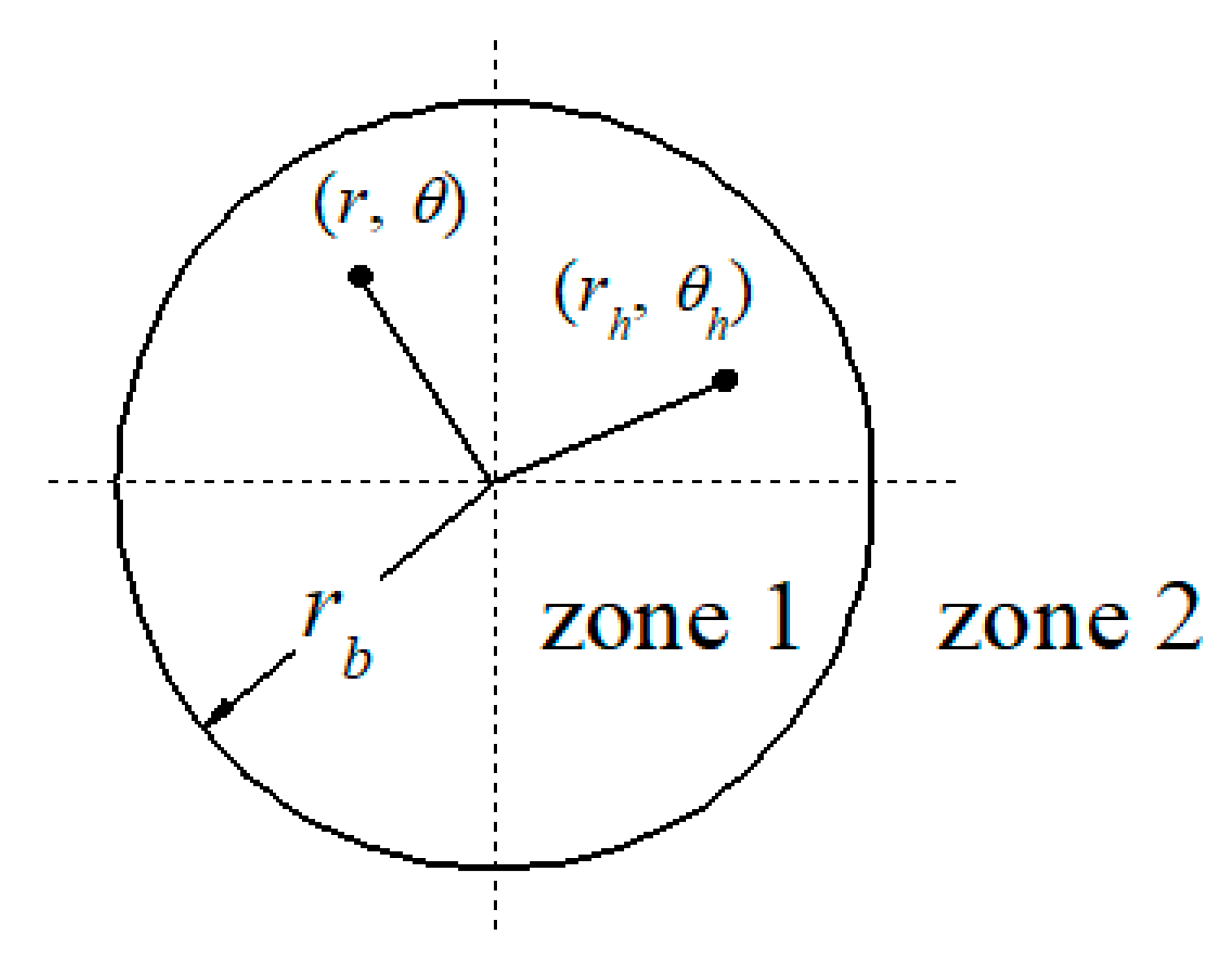
  • The radius of the borehole is rb, and depth is H. The properties of the grout and soil are homogeneous and isotropic. These properties include soil thermal conductivity λs, soil volume heat capacity cs, grout thermal conductivity λg, and volume heat capacity cg.
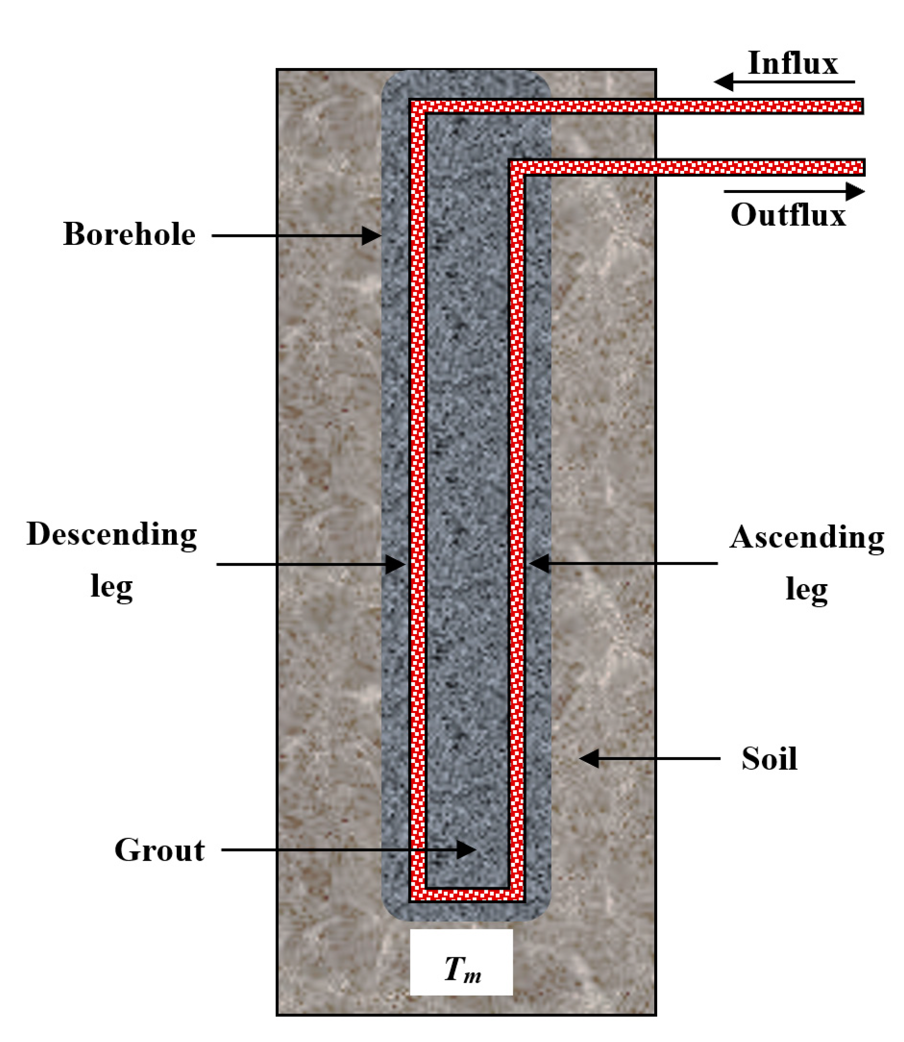
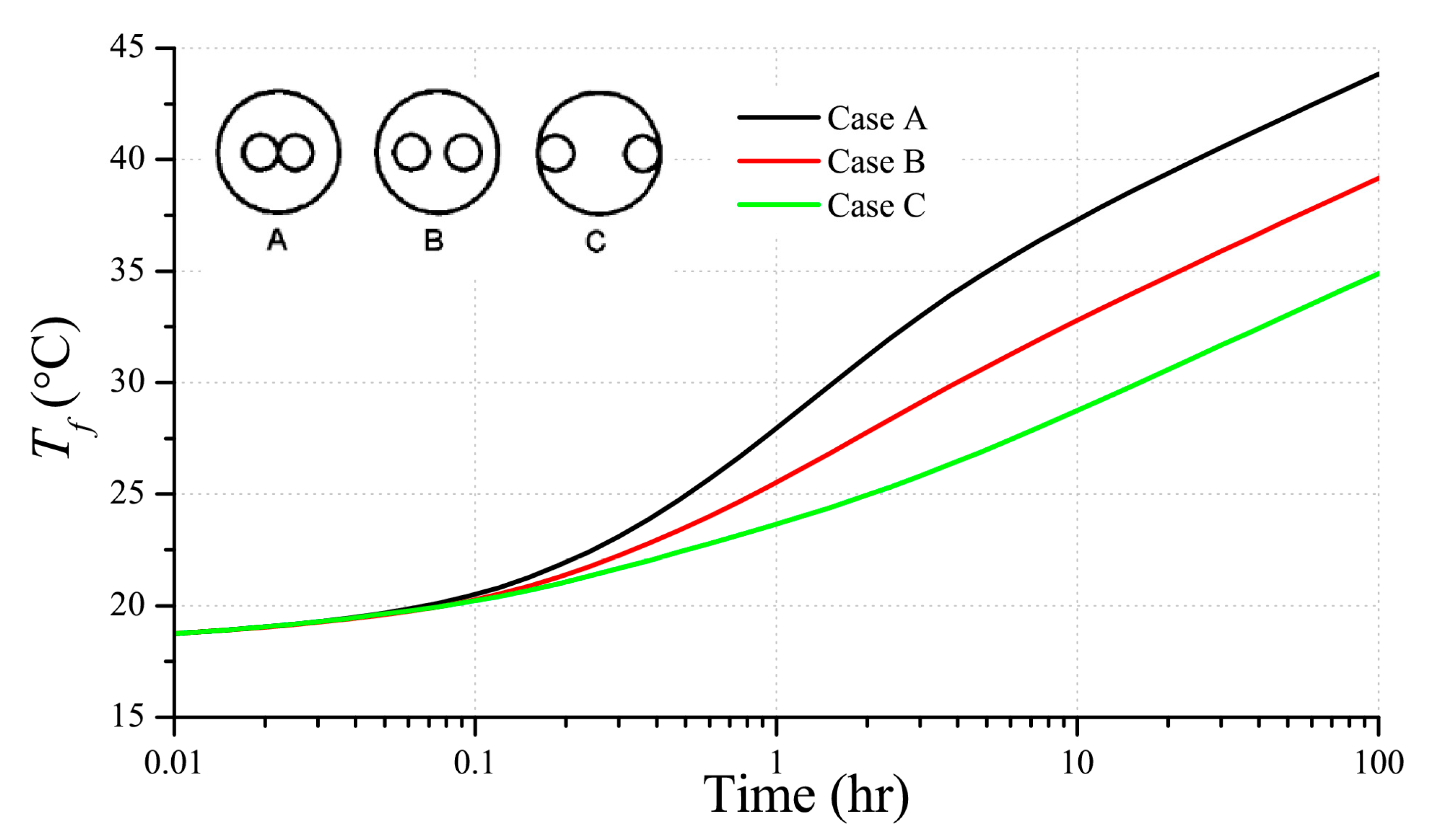
  • The two legs of the U-tube are symmetrically arranged with respect to the center of the borehole. The distance between the two legs is 2D. The fluid is pumped into the descending leg with an inlet temperature Tin, and flows out of the ascending leg with an outlet temperature Tout. The temperature at the bottom of the U-tube is Tm. The average heat rates of the descending leg and ascending leg are qp1 and qp2, respectively.
  • The total heat rate of the GHE qG is assumed to be a constant. The fluid flows in the tube with a constant volumetric flow rate wf, the volume heat capacity of the fluid is cf, and the average heat rates of fluid in the two legs are qf1 and qf2, respectively. Thus, we can have:
    q G = q f 1 + q f 2
The fluid flow in the tubes is turbulent, and the heat transfer along the vertical direction can be neglected.

2.2. Composite Line Source Model

The detailed formulation of the 2-D composite line source model is presented in Appendix A and Appendix B. In order to account for the fluid storage effect, both heat rates of the two legs, qf1 and qf2, will vary with time. Therefore, it can be more convenient to develop the model in the Laplace domain [15,17]. The Laplace transform of function f(t) is given as [20,21]:
f ¯ ( s ) = 0 t f ( t ) · e s t d t
where the overbar “-” denotes functions in Laplace space, and s is Laplace transform variable.
Based on the average fluid temperature equations (Equations (A6) and (A7)) of the two legs, we can obtain the following equations for characterizing the heat rates of the descending leg and the ascending leg:
q ¯ f 1 q ¯ f 2 = ( 1 + s ω f · α α ) · ( T ¯ f 1 T ¯ f 2 )
q ¯ f 1 + q ¯ f 2 = ( 1 + s ω f · β β ) · ( T ¯ f 1 + T ¯ f 2 )
where s is the Laplace variable and ωf is the fluid thermal storage coefficient. The coefficients α and β are defined as:
{ α = s T ¯ u 11 s T ¯ u 12 + R t / H β = s T ¯ u 11 + s T ¯ u 12 + R t / H
Substituting Equation (A12) into Equation (5), we can obtain the heat rate difference between the two legs:
q ¯ f 1 q ¯ f 2 = q G s 1 c f w f 1 + s ω f · α 2 α
With the aid of Equation (3), the heat rates for the descending and ascending legs can be written as:
{ q ¯ f 1 = q G 2 s · ( 1 + 1 c f w f 1 + s ω f · α 2 α ) q ¯ f 2 = q G 2 s · ( 1 1 c f w f 1 + s ω f · α 2 α )
Substituting the heat rates Equation (9) and Equation (8) into Equation (A13), we can readily obtain the average fluid temperature of the GHE:
T ¯ f = T ¯ i n + T ¯ o u t 2 = q G 2 s · ( β 1 + s ω f · β + 1 4 ( c f w f ) 2 1 + s ω f · α α )
Although the above solutions are formulated in Laplace-domain, we can easily obtain the time-domain solutions with the Stehfest numerical inversion method [22].

3. Results and Discussion

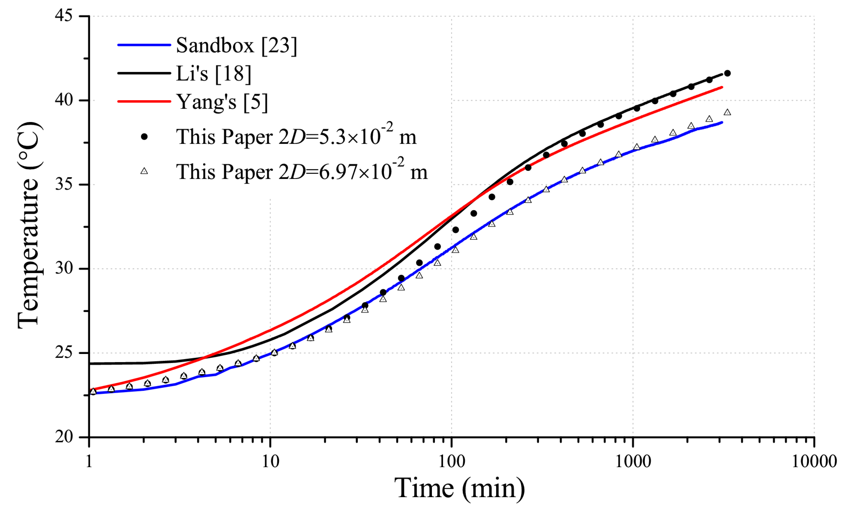
3.1. Model Verification

Beier [23] obtained reference data from a sandbox experiment which can be used to verify the developed heat transfer model. Moreover, this proposed model is validated against the analytical method from Li et al. [18], as well as the numerical model from Yang et al. [5]. The values of the Parameters of the sandbox experiment are listed in Table 1.
Figure 2 presents the comparison between the results of our model and those of the other models, as well as the reference data. It can be observed in this figure, compared with the results of the two existing models, this new model has a better agreement with the reference data during the early period. While for the late period, the results from the new model illustrate a similar trend to those from Li’s model and Yang’s model. Besides, as suggested by Beier et al. [24], the distance between the legs can be a function of depth rather than a constant. As shown in Figure 2, a better agreement can be achieved for the entire test duration with a modified average distance 2D = 6.97 × 10⁻² m. Therefore, the excellent agreements imply that this proposed model is reliable for simulating the thermal behavior of the single U-tubes.

3.2. Early Thermal Response Analysis

In this section, the effects of fluid thermal storage, fluid flow rate, and the distance between the two legs are examined with the new composite-medium line source model. The benchmark values of the parameters are listed in Table 2

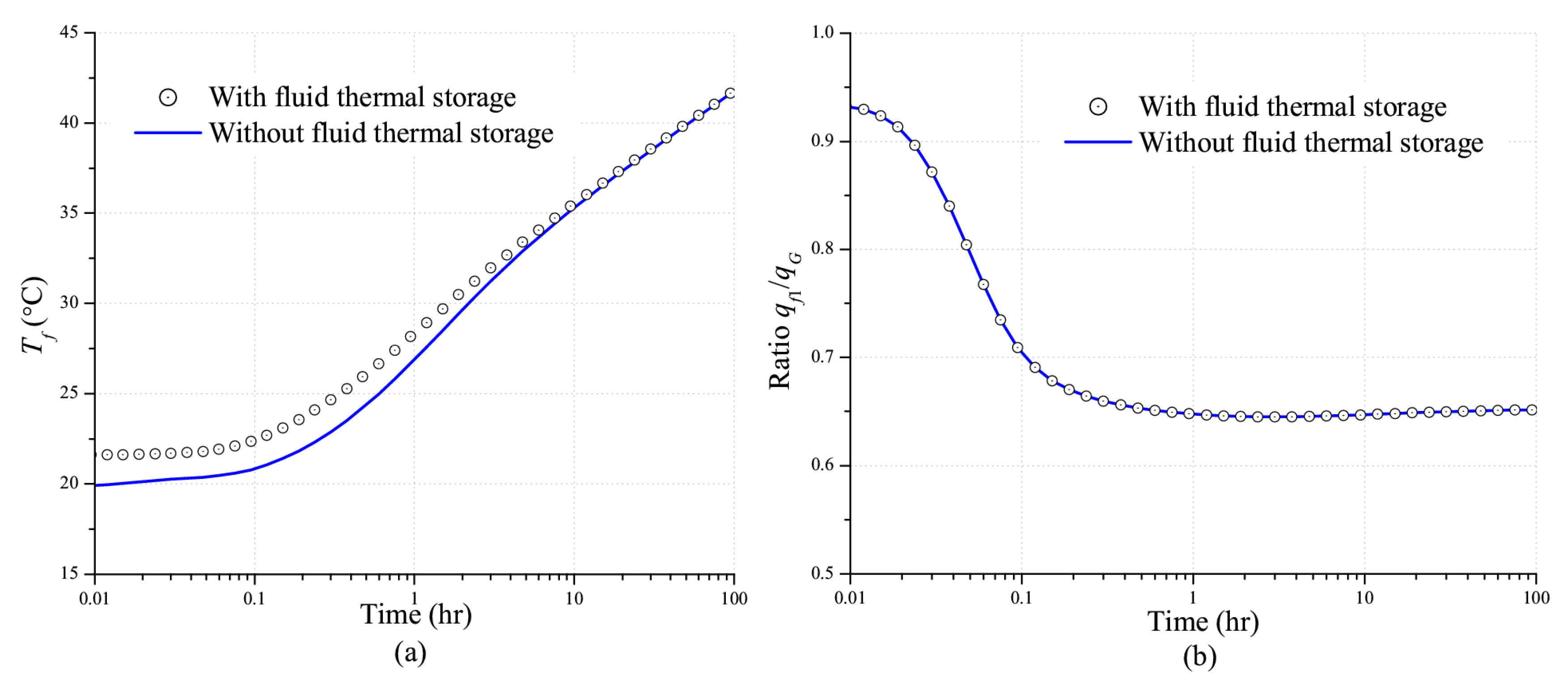
3.2.1. Effect of Fluid Thermal Storage

Figure 3 compares the calculated temperature and heat ratio that consider the fluid thermal storage to the calculated temperature and heat ratio that neglect the fluid thermal storage. As shown in Figure 3a, the fluid thermal storage mainly exhibits its influence at the early time. The calculated temperature that considers fluid thermal storage is lower than that of those neglecting the fluid thermal storage. The difference between the two temperature plots becomes more pronounced at the early time. This is because the heat rate mainly contributes to the temperature promotion of the fluid inside the tube at the early stage. As time proceeds, the effect of fluid thermal storage fades.
Figure 3b presents the ratio of the heat rate of the descending leg to the total heat rate. As one can see in this figure, the heat rates of the two legs are different. The heat ratio is larger than 0.5 throughout the entire simulation period, which indicates that the heat rate of the descending leg is higher than that of the ascending leg. The value of the ratio decreases and it approaches a constant value in the late period. In addition, it can be found that the difference between these two plots is negligible, which implies that the fluid thermal storage exerts a slight effect on the heat rate distribution.

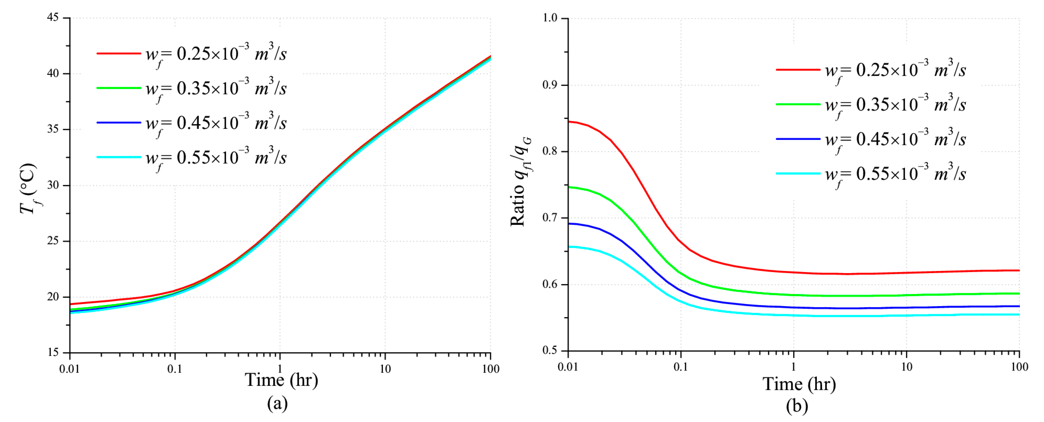
3.2.2. Effect of Fluid Flow Rate

Figure 4 presents the effect of flow rate on the thermal behavior of a single U-tube. In Figure 4a, the difference between the average temperature with different flow rates is not significant during the late period. A more noticeable difference can be observed during the early period. This is because the second term in Equation (10) is very sensitive to the flow rate, which is reciprocal to the square flow rate. In Figure 4b, one can see that the flow rate can significantly influence the heat rate distribution between these two legs. As shown in Figure 4b, with a higher flow rate, the descending leg will contribute less to the GHE and the change of ratio is less significant on each plot.

3.2.3. Effect of Distance between the Two Legs

The distance between the two legs can affect the thermal behavior of the GHEs. Three typical cases [12] for different distances between the center of the two legs are studied with the new composite-medium line source model. Figure 5 presents the calculated results of the three cases with the proposed model. In Figure 5, one can see that that the distance between the two legs has a negligible effect during the early time when the fluid thermal storage effect dominates. However, the differences become significant at late simulation time. Since a smaller distance between the two legs can lead to a higher thermal interference, the fluid temperature is decreased as the case is varied from A to C. This implies the two legs should be installed as far as possible to reduce the thermal interference between two legs.

4. Conclusions

In this work, we proposed a new composite-medium line source model for modeling the thermal response of GHEs with a single U-tube. The new model is developed in Laplace space and solved with the numerical Laplace inversion method. Compared with the previous composite-medium line source models, the new model can be used to study the effect of fluid flow storage effect, as well as the heat rate difference between the two legs. The new composite-medium model is validated with reference data from the experiment and simulation results of existing models. It is worth noting that the heat transfer along the vertical direction is neglected in this work. In real field cases, if the temperature variation along the vertical direction is significant, one should utilize a 3D model to handle such a scenario.
The heat rate of the two legs are different, and the contribution of the descending leg to the GHE becomes smaller by increasing the flow rates. The fluid thermal storage has a significant influence on the early-time thermal transient response. Therefore, the effect of fluid thermal storage should not be neglected when one studies the thermal transient behavior in the borehole. The thermal interference between the two legs will reduce the heat capacity of GHEs. A larger distance between these two legs can be preferred for practical use.

Author Contributions

Conceptualization, S.G. and C.T.; methodology, S.G.; validation, J.H.; formal analysis, W.L.; investigation, S.G. and C.T.; data curation, W.L.; writing—original draft preparation, J.H.; writing—review and editing, B.T.; funding acquisition, S.G. All authors have read and agreed to the published version of the manuscript.

Funding

This research was funded by RESEARCH ON 3D SEISMIC ANISOTROPY ANALYSIS AND SWEET SPOT RESERVOIR PREDICTION TECHNOLOGY BASED ON SINGLE SANDBODY, grant number 2016ZX05050.

Conflicts of Interest

The authors declare no conflict of interest.

Nomenclature

2DDistance between centers of pipe, m
HLength of borehole, m
ttime, s
sLaplace variable with respect to time t
s ˜ Laplace variable with respect to dimensionless time tD
rradius or radial distance, m
Rthermal resistance, m∙K/W
T0initial ground temperature, °C
Ttemperature, °C
Tuline source function
cvolumetric specific heat, J/(K∙m3)
qheat rate, W
wvolumetric flow rate, L/s
Sdistance, m
Kn/Inthe modified Bessel functions of the nth order of the first and second kinds
bborehole
ffluid
ggrout
hheat source
piinner of pipe
poouter of pipe
ppipe
ssoil
ttotal
ininlet
outoutlet
Ddimensionless
Gground heat exchanger
1/2descending/ascending leg of the single U-tube, inner/outer region
ωfluid thermal storage coefficient, J/K
αcoefficient
βcoefficient
λthermal conductivity, W/(K∙m)
θangle

Appendix A. Composite-Medium Line Source Model for Ground Heat Exchangers with a Single U-Tube

Appendix A.1. The Average Temperature of the Fluid Inside the Two Legs

In the new analytical models, the two legs of the single U-tube are treated as two separate infinite line sources in the composite medium. The interference between the two legs can be described with the superposition principle. In order to account for the fluid thermal storage and heat rate difference between the two legs, the heat rates qf1 and qf2 are not constant. Therefore, the fluid temperatures Tfi inside the two legs should be written in the following convolution form [21]
T f i ( t ) = 0 t q p 1 ( τ ) · d T u i 1 d t ( t τ ) d τ + 0 t q p 2 ( τ ) · d T u i 2 d t ( t τ ) d τ + q p i ( t ) · R t H ,   i = 1 ,   2
where Tu is the temperature response with respect to the composite-medium line source model. Subscript “ij” denotes the effect of i-th to the j-th leg. The thermal resistance Rt inside the tube can be written as:
R t = R t p + R t h
where Rtp is the conductivity thermal resistance of pipe, Rth denotes the convective thermal resistance between the fluid and pipe wall. Beier and Smith [15] presented detailed algorithms for calculating Rtp and Rth. In the Laplace domain, Equation (A1) with convolution, integrals can be rewritten as:
T ¯ f i ( s ) = q ¯ p 1 ( s ) · s T ¯ u i 1 ( s ) + q ¯ p 2 ( s ) · s T ¯ u i 2 ( s ) + q ¯ p i ( s ) · R t H ,   i = 1 ,   2
Furthermore, the heat rates of the pipe walls are given as:
q p i = q f i ω f · d T f i / d t
Considering the fluid thermal storage coefficient:
ω f = π r p i 2 H · c f
Transforming Equation (A4) into Laplace space and substituting it into (A3) we can obtain fluid temperature equations. For the descending leg we can have:
[ 1 + s ω f · ( s T ¯ u 11 + R t H ) ] · T ¯ f 1 + s ω f · s T ¯ u 12 · T ¯ f 2 = q ¯ f 1 · s T ¯ u 11 + q ¯ f 2 · s T ¯ u 12 + q ¯ f 1 · R t H
For the ascending leg, we can have:
s ω f · s T ¯ u 12 · T ¯ f 1 + [ 1 + s ω f · ( s T ¯ u 11 + R t H ) ] · T ¯ f 2 = q ¯ f 1 · s T ¯ u 12 + q ¯ f 2 · s T ¯ u 11 + q ¯ f 2 · R t H
In addition, with the infinite line source assumption, the average fluid temperatures for the two legs can be written as
{ T f 1 = T i n + T m 2 T f 2 = T o u t + T m 2

Appendix A.2. Equations of Inlet and Outlet Fluid Temperature

According to the conservation law, we can have the following equations of inlet and outlet fluid temperature. For the GHE:
c f w f · ( T i n T o u t ) = q G
for the descending leg:
c f w f · ( T i n T m ) = q f 1
for the ascending leg:
c f w f · ( T m T o u t ) = q f 2
Combined Equation (A8) with Equations (A10) and (A11), we can obtain following average fluid temperature equation:
T f = T i n + T o u t 2 = T f 1 + T f 2 2 + q f 1 q f 2 4 c f w f

Appendix B. Temperature Response Function in a Composite Medium

Figure A1 shows an infinite composite cylinder consisting of two regions with depth H, the inner region r < rb with λ1 and c1, and the outer region r > rb with λ2 and c2. The initial temperature of the medium is 0 °C. An infinite line source of heat is located at (rh, θh), where r < rb and continuously releases heat into the composite medium from t = 0. Chen and Raghavan [25] provided an analogous pressure response functions for oil well in an infinite composite medium. The Laplace transformation of the temperature responses at a point (r, θ) located in the inner and outer regions are given by Equations (A13) and (A14), respectively.
Figure A1. Schematic layout of a line source positioned in an infinite composite medium.
Energies 13 02120 g0a1
For 0 < rrb
T ¯ u 1 ( s ˜ , θ , r D ) = 1 s ˜ q 2 π λ 1 H · { K 0 ( S D · s ˜ c D λ D ) ( A 0 E 0 · I 0 ( r D · s ˜ c D λ D ) · I 0 ( r h D · s ˜ c D λ D ) ) 2 · n = 1 + A n E n · I n ( r D · s ˜ c D λ D ) · I n ( r h D · s ˜ c D λ D ) · cos ( n | θ θ h | ) }
For r > rb:
T ¯ u 2 ( s ˜ , θ , r D ) = 1 s ˜ q 2 π λ 1 H · { B 0 E 0 · K 0 ( r D s ˜ ) · I 0 ( r h D · s ˜ c D λ D ) + 2 · n = 1 + B n E n · K n ( r D s ˜ ) · I n ( r h D · s ˜ ω D λ D ) · cos ( n | θ θ h | ) }
where
A n = c D λ D · K n ( r b D s ˜ ) · K n ( r b D s ˜ c D λ D ) 1 λ · K n ( r b D s ˜ c D λ D ) · K n ( r b D s ˜ )
B n = c D λ D · [ K n ( r b D s ˜ c D λ D ) · I n ( r b D s ˜ c D λ D ) I n ( r b D s ˜ c D λ D ) · K n ( r b D s ˜ c D λ D ) ]
E n = c D λ D · K n ( r b D s ˜ ) · I n ( r b D s ˜ c D λ D ) 1 λ · I n ( r b D s ˜ c D λ D ) · K n ( r b D s ˜ )
S D = r D 2 + r h D 2 2 · r D r h D cos | θ θ h |
and the dimensionless parameters as defined as:
λ D = λ 1 λ 2 ,   c D = c 1 c 2 ,   r D = r r p o ,   r b D = r b r p o ,   r h D = r h r p o ,   S D = S r p o .
In Equations (A13)–(A17), s ˜ is the Laplace variable with respect to dimensionless time tD,
t D = λ 2 c 2 r p o 2 t
The subscripts 1 and 2 denote inner regions (r < rb) and outer regions (r > rb); In and Kn are the modified Bessel functions of the nth order of the first and second kinds, respectively. The symbol “’” denotes derivatives. The modified Bessel functions have following equations,
K n 1 ( z ) = ( 2 n / z ) · K n ( z ) + K n + 1 ( z )
I n 1 ( z ) = ( 2 n / z ) · I n + I n + 1
Therefore, the functions Kn(z) and In(z) are computed recursively after computing K0(z), K1(z), I0(z) and I1(z). Moreover, their derivatives can be calculated with the following equations,
K n = K n 1 + K n + 1 2 ,   K n = K n
I n = I n 1 + I n + 1 2 ,   I n = I n

References

  1. Rees, S. Advances in Ground-Source Heat Pump Systems; Woodhead Publishing Ltd.: Cambridge, UK, 2016. [Google Scholar]
  2. Yang, H.; Cui, P.; Fang, Z. Vertical-borehole ground-coupled heat pumps: A review of models and systems. Appl. Energy 2010, 87, 16–27. [Google Scholar] [CrossRef]
  3. Li, M.; Lai, A.C.K. Review of analytical models for heat transfer by vertical ground heat exchangers (GHEs): A perspective of time and space scales. Appl. Energy 2015, 151, 178–191. [Google Scholar] [CrossRef]
  4. Yavuzturk, C.; Spitler, J.D. A short time step response factor model for vertical ground loop heat exchangers. ASHRAE Trans. 1999, 105, 475–485. [Google Scholar]
  5. Yang, Y.; Li, M. Short-time performance of composite-medium line-source model for predicting responses of ground heat exchangers with single U-tube. Int. J. Therm. Sci. 2014, 82, 130–137. [Google Scholar] [CrossRef]
  6. Javed, S.; Claesson, J. New analytical and numerical solutions for the short-term analysis of vertical ground heat exchangers. ASHRAE Trans. 2011, 117, 3–12. [Google Scholar]
  7. Ingersoll, L.R.; Zobel, O.J.; Ingersoll, A.C. Heat Conduction with Engineering, Geological, and Other Applications, revised ed.; The University of Wisconsin Press: Madison, WI, USA, 1954. [Google Scholar]
  8. Hellstrom, G. Ground Heat Storage: Thermal Analyses of Duct Storage Systems 1: Theory; Department of Mathematical Physics, University of Lund: Lund, Switzerland, 1991. [Google Scholar]
  9. Kavanaugh, S.P. Simulation and Experimental Verification of Vertical Ground Coupled Heat Pump Systems. Ph.D. Thesis, Oklahoma State University, Stillwater, OK, USA, 1985. [Google Scholar]
  10. Claesson, J.; Dunand, A. Heat Extraction from the Ground by Horizontal Pipes: A Mathematical Analysis; Swedish Council for Building Research: Stockholm, Sweden, 1983. [Google Scholar]
  11. Gu, Y.; O’Neal, D.L. Development of an equivalent diameter expression for vertical U-tubes used in ground-coupled heat pumps. ASHRAE Trans. 1998, 104, 347–355. [Google Scholar]
  12. Paul, N.D. The Effect of Grout Thermal Conductivity on Vertical Geothermal Heat Exchanger Design and Performance. Master’s Thesis, South Dakota State University, Brookings, SD, USA, 1996. [Google Scholar]
  13. Javed, S.; Spitler, J. Accuracy of borehole thermal resistance calculation methods for grouted single U-tube ground heat exchangers. Appl. Energy 2017, 187, 790–806. [Google Scholar] [CrossRef]
  14. Claesson, J.; Hellstrom, G. Multi-pole method to calculate borehole thermal resistances in a borehole heat exchanger. HVAC R Res. 2011, 17, 895–911. [Google Scholar]
  15. Beier, R.A.; Smith, M.D. Minimum duration of in-situ tests on vertical boreholes. ASHRAE Trans. 2003, 109, 475–486. [Google Scholar]
  16. Gu, Y.; O’Neal, D.L. An analytical solution to transient heat conduction in a composite region with a cylindrical heat source. J. Sol. Energy Eng. 1995, 117, 242–248. [Google Scholar] [CrossRef]
  17. Lamarche, L.; Beauchamp, B. New solutions for the short-time analysis of geothermal vertical boreholes. Int. J. Heat Mass Transf. 2007, 50, 1408–1419. [Google Scholar] [CrossRef]
  18. Li, M.; Lai, A.C.K. New temperature response functions (G functions) for pile and borehole ground heat exchangers based on composite-medium line-source theory. Energy 2012, 38, 255–263. [Google Scholar] [CrossRef]
  19. Li, M.; Lai, A.C.K. Analytical model for short-time responses of ground heat exchangers with U-tubes: Model development and validation. Appl. Energy 2013, 104, 510–516. [Google Scholar] [CrossRef]
  20. Abramowitz, M.; Stegun, I.A. Handbook of mathematical functions with formulas, graphs, and mathematical tables, national bureau of standards. Appl. Math. Ser. 1964, 55, 484. [Google Scholar]
  21. Carslaw, H.S.; Jaeger, J.C. Conduction of Heat in Solids, 2nd ed.; Claremore Press: Oxford, UK, 1959. [Google Scholar]
  22. Stehfest, H. Algorithm 368: Numerical inversion of Laplace transforms. Commun. ACM 1970, 13, 47–49. [Google Scholar] [CrossRef]
  23. Beier, R.A.; Smith, M.D.; Spitler, J.D. Reference data sets for vertical borehole ground heat exchanger models and thermal response test analysis. Geothermics 2011, 40, 79–85. [Google Scholar] [CrossRef]
  24. Beier, R.A. Vertical temperature profile in ground heat exchanger during in-situ test. Renew. Energy 2011, 36, 1578–1587. [Google Scholar] [CrossRef]
  25. Chen, C.; Raghavan, R. Modeling a Fractured Well in a Composite Reservoir. SPE Form. Eval. 1995, 10, 241–246. [Google Scholar] [CrossRef]
Figure 1. Schematic of a borehole GHE with a single U-shape tube.
Energies 13 02120 g001
Figure 2. Comparisons of the average fluid temperatures between the results of the proposed model and those of Li’s model, Yang’s model, and experimental data.
Energies 13 02120 g002
Figure 3. Thermal response plots calculated with the proposed model with different ωf: (a) average temperature of the fluid; and (b) ratio of the heat rate of the descending leg.
Energies 13 02120 g003
Figure 4. Thermal response plots of the U-tube with different flow rates: (a) average temperature of the fluid; and (b) ratio of the heat rate of the descending leg.
Energies 13 02120 g004
Figure 5. Thermal response of the U-tube with different distances between the two legs (Case A: 2D = 2rpo; Case B: 2D = rb; Case C: 2D = 2rb − 2rpo).
Energies 13 02120 g005
Table 1. Values of the parameters used for validating the proposed model [23].
ParametersSymbolValue
Initial ground temperatureT022 °C
Borehole radiusrb0.063 m
Length of boreholeH18.3 m
Outer radius of U-tube,rpo0.0167 m
Inner radius of U-tuberpi0.013665 m
Distance between centers of pipe2D0.053 m
Thermal conductivity of pipeλp0.39 W/(K∙m)
Thermal conductivity of soilλs2.82 W/(K∙m)
Volumetric heat capacity of soilcs3.2 × 106 J/(K∙m3)
Thermal conductivity of groutλg0.73 W/(K∙m)
Volumetric heat capacity of groutcg3.8 × 106 J/(K∙m3)
Volumetric heat capacity of the fluidcf4.19 × 106 J/(K∙m3)
GHE heat rateqG1053 W
Fluid volumetric flow ratewf0.197 L/s
Table 2. Benchmark values of the parameters of GHE with a single U-tube.
ParametersSymbolValue
Initial ground temperatureT018 °C
Borehole radiusrb0.75 m
Length of boreholeH120 m
Outer radius of U-tube,rpo0.016 m
Inner radius of U-tuberpi0.013 m
Distance between centers of pipe2D0.050 m
Thermal conductivity of pipeλp0.4 W/(K∙m)
Thermal conductivity of soilλs1.5 W/(K∙m)
Volumetric heat capacity of soilcs2 × 106 J/(K∙m3)
Thermal conductivity of groutλg0.9 W/(K∙m)
Volumetric heat capacity of groutcg2 × 106 J/(K∙m3)
Volumetric heat capacity of the fluidcf4.19 × 106 J/(K∙m3)
GHE heat rateqG6000 W
Fluid volumetric flow ratewf2.5 × 10−7 m3/s

