Abstract
This paper proposes and develops a circuit-based model aiming to simulate variable magnetic power elements in power electronic converters. The derived model represents the magnetic element by a reluctance-based equivalent circuit. The model takes into consideration device core losses, with the main emphasis given to hysteresis losses, which are modeled using the Jiles-Atherton model. The core loss model is further validated on different ferromagnetic materials to prove its range of applicability. The winding losses of the magnetic device are also taken into consideration, which are obtained using Dowell empirical formulas. In addition, the frequency dependence of the device losses is also considered. The proposed modeling procedure has been applied to study and characterize a double E-core variable power inductor structure in a 1 kW SiC full bridge DC-DC converter. The procedure has been verified by comparing the simulation results to the experimental measurements, confirming the validity and accuracy of the full circuit-based model.
1. Introduction
Understanding the behavior of a magnetic device in a Power Electronic Converter (PEC) is essential to optimize the design and to foster the performance of the whole system. Variable magnetic elements allow for additional degrees of freedom in the design and control of PECs. This is particularly useful in resonant converters where the usual frequency control has some drawbacks due to Electro-Magnetic Interference (EMI) issues, synchronization, variable sampling time, etc., especially for a large range of variation. If variable magnetics are used, the same control margins can be obtained at a constant switching frequency, therefore allowing for an optimization of the EMI filters and sampling procedures. In other applications, such as the Dual-Active-Bridge (DAB) converter, in addition to adding a new degree of freedom to the control, the inclusion of variable magnetics can increase operation parameters, such as the soft switching margins [1,2,3].
The recent growing applications of variable magnetic elements have implied the need for developing accurate models to define the magnetic device behavior. The magnetic core as well as the device windings must be characterized to achieve an accurate device model.
Some models define the magnetic core material in terms of a relationship between magnetic flux density and field intensity referred to as a hysteresis curve. In [4], an initial survey has been conducted classifying the existing magnetic material models, according to different frequencies, bias conditions, and temperatures of interest. It aims to provide comparable information for models and their availability in some circuit simulators. More recently, a literature review on the fundamentals, modeling, and design of magnetic regulators has been comprehensively presented in [5]. After a careful review of these and other references, the modeling methods are confined to analytical and numerical methods. Specific to variable magnetic devices, modeling strategies are confined to three directions: Finite Elements Analysis (FEA), gyrator-capacitor model [6], and reluctance equivalent circuit [7]. The FEA model is based on the numerical method, while the gyrator-capacitor model and the reluctance model are based on the analytical method.
As the complexity of magnetic devices increases, the analytical method becomes too complicated to predict the behavior of the device in a simple and practical manner. Therefore, incorporating those concepts in a computer-based simulation provides a good compromise between convenience, accuracy, and numerical efficiency. On the other hand, developing such simulations enables real-time applications on the modeling at the converter controller level, which can provide an on-line calculation of model parameters for real-time control [8]. Consequently, many efforts have been directed towards computer-based simulations, especially time-domain models [9,10]. Although the analytical methods of calculation are generally known and can be implemented in simulation models in a straight-forward manner, the selection of the suitable methods is critical from the circuit simulation perspective. The computation methods are expected to achieve good convergence with an acceptable compromise of accuracy to the time of processing the simulation results.
Henceforth, the aim of this work is to develop a circuit-based time-domain model of the variable magnetic element. The proposed model includes the device losses, mainly core and winding losses. Also, this circuital model is able to work in different platforms, for e.g., LTSpice® (Linear Technology Corporation, Milpitas, CA, USA) [11], MATLAB-Simulink® (MathWorks, Natick, MA, USA) [12], and PSIM® (Powersim Inc., Rockville, MD, USA) [13], with equally valid accuracy. Thereby, the whole electromagnetic system design and simulation can be carried out using only one simulator environment. This provides an acceptable accuracy in compromise with the complication and time required for FEA models. Consequently, it allows the investigation of the overall PEC performance incorporating the variable magnetic device. Section 2 presents an overview of the variable magnetic device structure that will be used, together with the models of interest in the literature. In Section 3, the magnetic core losses are studied and the method used to model those losses is presented. This section also provides an idea on the implementation of the model equations, the validation of the model against experimental measurement, and the approach to estimate the model parameters as a function of the operation frequency. Later, in Section 4, the model of the winding losses is presented, and validated against experimental results. After that, Section 5 explains the use of the loss models to implement the full device model. In Section 6, the proposed simulation model is validated in comparison to the previous models that does not include losses, and experimental results are provided. Finally, Section 7 summarizes the conclusions of the work.
2. Modeling of Variable Magnetic Elements
From the study of the state of the art, the double E-core structure, depicted in Figure 1, is selected to be the most appropriate for the implementation of the variable inductor in this study and the most comprehended in literature [14]. The basic principle of operation of a double E-core variable inductor is described in this section.
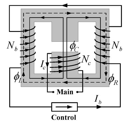
Figure 1.
Variable inductor based on a double E-core structure.
Due to the current () flowing through the main winding () of the inductor, as clarified in Figure 1, an AC flux () circulates through the center arm of the typical E-core structure of the magnetic core and splits to the outer arms. Applying a relatively small DC current () to the bias control windings (), a DC flux ( or ) is produced, which circulates mainly through the outer (ungapped) closed path of the core [14]. This DC flux can bias the operation of the magnetic material towards the nonlinear region on the curve, thus causing the inductance seen from the main winding terminals to vary as a function of the DC bias current, Equation (1).
In order to model the variable magnetic device, the operation regions of the magnetic material on the curve must be considered. These are divided into three areas: the linear region, the saturation knee, and the non-linear region [9].
In addition, to attain accurate results in the modeling procedure, the different involved device losses are included. There are two main types of losses associated to the magnetic device; core losses and winding losses. For MnZn-ferrite materials, the core losses are composed of three fractions. A fraction of the losses is related to the crystal composition, which is called hysteresis losses. Another fraction is related with the structural form of the core, which is called eddy current losses. As the frequency increases, the eddy currents dominate, and for a frequency range of approximately 1 MHz, those losses can contribute with more than 50% of the total power losses. There is also a third fraction known as resonance losses [15]. This fraction is related to the ferrimagnetic resonance of the material and is pertinent to both the crystal and microstructure.
On the other hand, the winding losses depend on the frequency of operation of the magnetic device. At DC operation, the winding losses are due to the resistance of the copper wire. However, as the frequency of operation increases, two effects take place, which are the skin and the proximity effects. Those effects cause the wire resistance to vary, and this modified resistance is referred to as the AC (or high-frequency) winding resistance.
Although ready-made modules are available in many circuit simulation environments [12,13], it is not considered comprehensive to study the magnetic device. The SPICE-based reluctance equivalent circuit provided by authors in [9] is, thus, found to be of more interest. Figure 2 shows the reluctance equivalent circuit for the double E-core variable inductor.
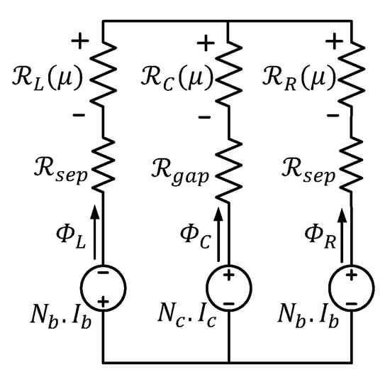
Figure 2.
Reluctance equivalent circuit of the double E-core variable inductor shown in Figure 1.
The voltage sources in the circuit represent the magnetomotive forces due to the bias control windings (), as well as the main winding (). is a constant reluctance that represents the air gap, while is a constant reluctance that represents the air separation between the two E-cores due to non-idealities in the manufacturing process. The components , , and are the reluctances of the magnetic paths of the left, center, and right arms, respectively. These reluctance values are represented as a function of the permeability of the magnetic material (), and it must be noticed that, unlike the usual case, in variable magnetic elements, these permeability values can vary depending on the operation point of the magnetic core material on the characteristic curve. Thus, for calculating these reluctances, the referred model uses Brauer’s equation [16], which defines the characteristic curve of the magnetic material neglecting the hysteresis effect, as stated by Equation (2).
where , , and are constants that depend on the considered magnetic material. For the present work, the afore-mentioned SPICE-based model has been replicated, specifically, in the MATLAB-Simulink® platform. This has been carried out in order to take advantage of the feature of this environment to integrate MATLAB script with existing Simulink® library tools, aiming to combine complex, accurate simulations with digital processing of information. This allows including the device design calculations into the overall model of the system in one integrated environment.
Two key limitations are found in this model, which restrict its applicability range and accuracy. Firstly, the hysteresis effect is not taken into consideration. Secondly, the model input quantities are dependent on the output ones, which introduces difficulty in the implementation of the computations. In particular, the latter issue implies the necessity for implementing system calculation delays, with an adequate initialization of parameters, especially when including the device in a switching converter simulation. This, furthermore, complicates the simulation in different test platforms. In Simulink®, for instance, the solver applies a numerical method to solve the set of ordinary differential equations that represent the model; therefore, the model causality must be decided [17].
In this paper, the model of the variable inductor has been extended to include device losses. The main loss components that have been taken into consideration are the hysteresis losses of the magnetic core and the winding losses. The following sections will justify the studied loss components and discuss the implementation and validation of the full model [18].
It is worth noting that, throughout the discussion hereafter, the vectorial nature of the magnetic quantities are disregarded to reduce the analysis to a simple unidimensional statement of equations by assuming: (1) specific symmetrical magnetic core geometries, of which geometrical references and paths are well-defined, and (2) the homogeneous nature of typical magnetic core materials together with the uniform distribution of the magnetic core properties. Such assumptions are often used in the analysis and design of magnetic devices for power electronics converters.
3. Model of Core Losses
The core losses in a magnetic core are due to two phenomena: the hysteresis loss, and the eddy currents loss. The hysteresis loss is due to energy required to rotate the magnetic domains when aligning with the applied magnetic field. On the other hand, the eddy current losses are due to currents induced in the magnetic core, which opposes the changing flux in the core. Previous studies in literature [19] have shown that for a ferrite magnetic material operating in a range of frequency up to 100 kHz, the eddy current losses are a very small part of the total core losses. Therefore, for the range of frequencies under study herein, the hysteresis losses will always be dominant. For this reason, the eddy current losses in the magnetic core will be neglected in this study for the sake of simplicity.
There are several methods to calculate the hysteresis losses in a ferro-magnetic material, which were grouped by the authors in [20] to be three main approaches: hysteresis models, empirical equations, and loss separation. This paper undertakes the first approach, specifically the Jiles-Atherton (JA) hysteresis model [21]. The main strengths of the JA model compared to its counterpart approaches are: being the most suitable for development from a circuital simulation perspective, besides having good convergence and acceptable accuracy among a variety of materials and operation conditions [22].
This section is dedicated to explaining in detail the model of core losses. First, the JA equations are defined and implemented using block diagram modeling in Simulink®. Second, a test setup is built for measuring the magnetic flux density and field intensity to validate the model in comparison to experimental measurements. Finally, to include the effect of the switching frequency on the core loss model, expressions are obtained for the JA parameters as a function of the switching frequency based on an empirical approach.
3.1. Model Implementation
The JA model separates the magnetization, M, into reversible, , and irreversible magnetizations, , which correspond to the reversible or irreversible phenomena, which take place within the magnetic material during the magnetization [22]. By computing the latter components, the total magnetization, M, is defined as the summation of both components as explained by Equation (3).
The reversible component of magnetization is defined as a fraction, c, of the difference of the anhysteretic magnetization and the irreversible one, as explained by Equation (4).
where c is referred to as the reversibility coefficient. The irreversible component of magnetization is defined by the differential Equation (5).
where k is the loss coefficient, and is the interdomain coupling. indicates the direction of the magnetizing field H, such that for increasing field, and for decreasing field, as defined by Equation (6).
is the anhysteretic magnetization. The anhysteretic magnetization describes the magnetization of an ideal ferromagnet that does not have a loss effect, and thus, its magnetization curve does not present hysteresis. Langevin’s function [23] is used within the JA model for defining the anhysteretic magnetization, in which case, an effective field, , replaces the magnetic field, H, as explained by Equation (7) [24].
where is the saturation magnetization, a is the shape parameter for anhysteretic magnetization, and is defined by Equation (8).
Consequently, the magnetic flux density can be calculated using Equation (9).
Table 1 summarizes the definition of the model parameters, , a, c, and k. The parameters are initially estimated by an iterative procedure to fit the model to the magnetic material curve data provided by the manufacturer.

Table 1.
Jiles-Atherton model parameters.
Figure 3 shows a block diagram of the detailed implementation of the JA equations [22]. Following this block diagram, the model equations have been implemented in Simulink®. Therefore, for a given core size and magnetic material, the instantaneous magnetic flux density (B) can be estimated for a certain instantaneous magnetic field intensity (H) applied to the magnetic core.
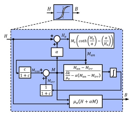
Figure 3.
Schematic of the implementation of the Jiles-Atherton (JA) model.
3.2. Test Setup for Measuring Core Losses
In order to validate the implemented JA model and study the effect of frequency on the model parameters, a test setup is developed. The purpose of the experiments is to measure the hysteresis losses of the magnetic core and compare it to the one obtained by the implemented JA model. In literature, mainly two approaches for measuring core losses can be found [25]: electrical methods, and calorimeter-based methods. One of the former approaches has been selected, which is the curve electrical measurement technique. Specific to the selected technique, the two-winding measurement method [26] is used since it is reported to be accurate for the frequency range under test in this study (<100 kHz) [27].
Figure 4 illustrates a schematic to clarify the test setup used for measuring the core losses, while Figure 5 shows the experimental platform developed.
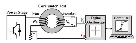
Figure 4.
Schematic diagram of the test setup used to measure the curve.
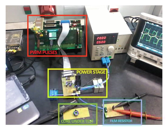
Figure 5.
Experimental setup used to measure the curve.
The power stage used in the tests is a simple half-bridge converter suitable for low power levels. A square-waveform excitation voltage is sought to verify the loss study under non-sinusoidal conditions. The core used for the identification tests is a toroidal core with the design parameters listed in Table 2. This toroidal geometry is used in order to ensure that the model results are not only valid for the selected double E-core structure but also for other geometrical schemes.
Table 2.
Specifications of the test setup developed to measure the curves.
In addition to the main excitation winding (), a secondary sensing winding () is added to sense the induced voltage due to the flux in the main one. The advantage of a separate winding is to exclude the voltage drop due to the resistance of the main winding. Therefore, the magnetic flux density can be computed using Equation (10).
where A is the cross-section area of the toroid, and is the open-circuit secondary winding voltage. The integration is performed over one switching period, T. The field intensity can, thus, be computed using Equation (11).
where is the current flowing through the main winding, and l is the effective length of the core. The measured voltage () and current () are illustrated in Figure 6a,b, respectively. By applying these measurements to Equations (10) and (11), the B and H quantities can be calculated. In this manner, the measured curve of the N87 magnetic material is compared to the curve obtained from the implemented JA model simulation under the same operation conditions. To apply the JA model, the model parameters are estimated by iterative fitting as mentioned previously, the obtained parameters for N87 magnetic material at 50 kHz are stated in Table 3. The resulting comparison is shown in Figure 7. It can be observed that the JA simulation model predicts the curve of the N87 magnetic material with an error of less than 5%. It can, thus, be concluded that the model is valid and provides acceptable accuracy. Furthermore, the model has been tested under different magnetic materials. The previous measurements were repeated at the exact same operation conditions while using a similar toroidal core from 3C90 magnetic material, the JA parameters of which are stated in Table 3. The B and H quantities were again measured, and the curves were compared together with the modeled ones, as illustrated in Figure 7. Similar to the previous results, the model shows a clear coincidence with the experimental measurements.
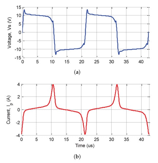
Figure 6.
Experimental measurements. (a) Voltage applied to the toroid, and (b) current flowing through the main winding.
Table 3.
Estimated Jiles-Atherton parameters for N87 and 3C90 magnetic materials at 50 kHz.
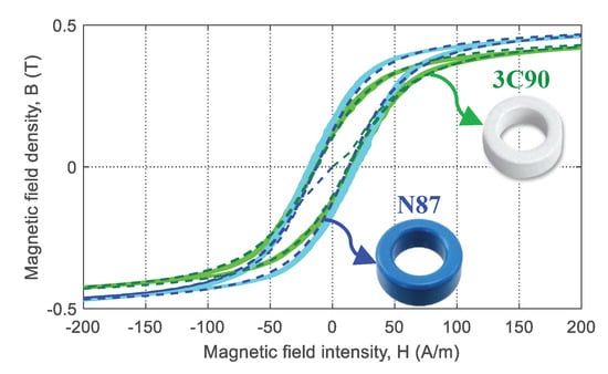
Figure 7.
Model (dotted line) versus experimental (solid line) curves for two different magnetic materials: N87 (blue) and 3C90 (green).
The hysteresis losses are estimated in terms of the area enclosed by the loop and, therefore, can be expressed as shown by Equation (12).
where is the core volume, and f is the switching frequency. The integral is performed over a complete cycle of the magnetic field intensity.
3.3. Frequency Dependence of JA Parameters
Since the behavior of the magnetic core material depends on the excitation frequency, different voltage waveforms in the magnetic element imply notable variations in the associated trajectories on the characteristic of the material. Specifically, it changes the area enclosed in the hysteresis loop, which is directly related to the core losses. This variation of the trajectory in itself implies a variation of the parameters of the JA model parameters. It is, thus, of interest to develop a model that can be used for any frequency without having to readjust the parameters each time different operating conditions are considered.
A practical approach has been taken by conducting a few experiments to characterize the variation of the JA model parameters as a function of the frequency. For the same core size and material, a number of independent tests were carried out, each test for a given frequency of operation. Then, a simple procedure is followed to obtain the parameters, as listed below:
- The instantaneous waveforms of the voltage () and the current (), as explained in the previous section, are captured.
- Fast Fourier Transform (FFT) is applied to these waveforms in order to identify the waveform frequency.
- For each test, the set of obtained JA model parameters is collected.
- Using curve fitting techniques (specifically the Curve Fitting Toolbox from Matlab®), an expression is obtained for each of the JA model parameters , , and as a function of switching frequency. The parameters c and show insignificant variation with frequency.
The expressions are intrinsic to a certain magnetic material. In this case, the procedure has been implemented for the N87 material; however, the same procedure can be followed for extracting a set of expressions for the JA parameters of any other ferrite material.
To test the validity of the obtained expressions for the JA parameters as a function of frequency, several experiments were carried out using the N87 toroidal core described in Table 2. The switching frequency of the converter was changed and the curves corresponding to different frequency values were measured and compared to the modeled ones, as illustrated in Figure 8. The results of the comparison show that the modeled curves match the obtained experimental measured curves at a wide range of the operation frequency with acceptable accuracy.
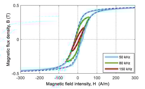
Figure 8.
curves for the prototype under different operation frequencies. Model (dotted line) versus experimental results (solid line).
4. Model of Winding Losses
4.1. Winding Eddy Current Losses
The winding losses are due to the resistance of the copper wire. At DC operation currents or relatively low operation frequencies, this resistance component is constant and calculated using Equation (16).
where is the resistivity of copper material at 20 C, which is equal to Ωm, is the total length of the winding wire, and is the cross-section area of the wire.
However, as the switching frequency increases, two effects start to appear, which are the skin effect and proximity effect. These effects induce eddy currents in the winding conductors, altering the resistance of the winding, and significantly contributing to the overall winding losses. It is necessary in this case to calculate the AC resistance of the winding. Dowell provided a method that computes the equivalent winding resistance using a one-dimensional analytical approach [28]. Initially, this method was intended to describe high-frequency loss in foil windings; however, it has been extended to multilayer windings with round conductors by introducing the porosity factor [28,29]. Dowell’s method uses a sinusoidal approach, and the calculations are limited to non-gapped cores [30]. On the other hand, the method presents a great advantage of simplicity and a fast computation of the AC winding resistance; thus, it can be easily integrated into the magnetic device model without extra complexity. Dowell estimates the AC resistance () by scaling the DC winding resistance by a factor, as shown in Equation (17).
where and are coefficients defined based on the geometrical dimensions of the winding, material characteristics, and frequency of operation, and m is the number of layers. The accuracy of the full winding model will be provided in the following sections to assess the validity of using Dowell’s method for the application herein.
4.2. Winding Stray Capacitance
As the operation frequency increases, the parasitic capacitance of the inductor winding becomes more significant, causing the impedance of the inductor to change and introduce the resonant frequencies. In order to attain a full comprehensive model of the device, the stray capacitance of the windings is added to the model. The calculation of the stray capacitance is based on an analytical approach previously presented in literature [31]. This method is valid for multi-layer inductors with ferromagnetic cores, as well as being simple and reliable for simulation purposes. Briefly, the inductor winding is divided into partitions, and the turn-to-turn and turn-to-core capacitances of the winding are predicted as a function of a few geometrical parameters of the device. Accordingly, the overall stray capacitance of the coil () converges to the expression stated in Equation (18).
where is the turn-to-turn capacitance of the coil and is defined by Equation (19).
where is the turn length, is the angular coordinate, and are the permittivity of air and relative permittivity of the insulation medium, respectively, and and are the diameters of the wire with and without the insulation coating, respectively, as clarified by Figure 9.
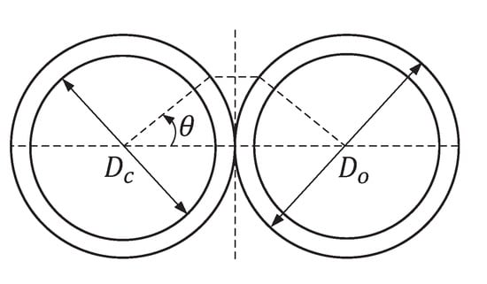
Figure 9.
Two adjacent turns of the winding.
4.3. Full Winding Model
The full model of the inductor winding is expressed by the circuit diagram in Figure 10. Therefore, the total impedance of the winding is calculated by Equation (20).
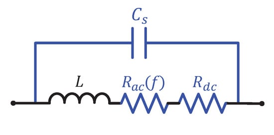
Figure 10.
Full winding model.
An inductor prototype was implemented based on the specifications summarized in Table 4. The inductance value is not of specific importance in the design; however, it is interesting to distribute the winding on several layers to emphasize the proximity effect. Figure 11 illustrates the total winding impedance as a function of frequency to compare the developed winding model against the experimental measurements. As it can be observed, the error between the measured and modeled impedances is less than 1%, which represents a quite high accuracy for the study in context.
Table 4.
Specifications of the inductor prototype developed to validate the winding model.
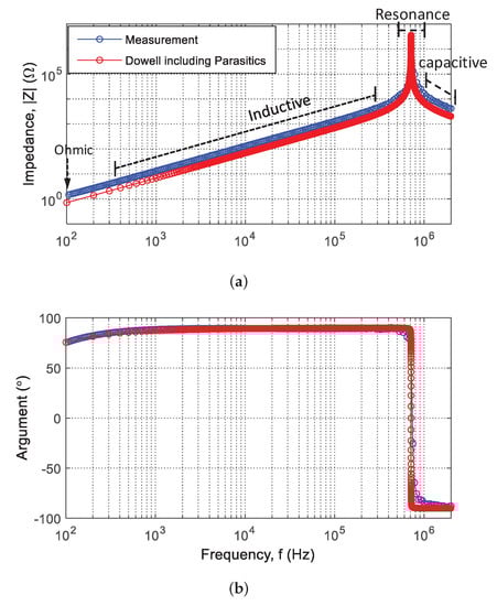
Figure 11.
Total winding impedance as a function of frequency. (a) Magnitude, and (b) argument of modeled impedance compared to experimental measurements.
5. Applications of Loss Models to Simulate the Variable Inductor
After the verification of the loss models, the study is applied to model the double E-core variable inductor shown in Figure 1. The full model is implemented based on the reluctance circuit concept previously stated. However, the two issues associated with the previous reluctance model have been tackled. To avoid algebraic loops due to model causality, the magnetic core has been partitioned according to its operation, as mentioned previously, in Section 2, thus defining each partition in terms of electrical inputs and outputs as explained below.
The middle arm has the main winding, and to model this arm, the input will be the excitation voltage, and the output should be the main inductor current. On the other hand, the lateral arms have the control windings, so for these coils, the input will be the control current, and the output should be the induced voltages in the control windings.
Figure 12a illustrates the magnetic system, which is represented by the reluctance equivalent circuit of the device. The reluctance equivalent circuit is composed of three branches. The left and right branches represent the magnetic circuits of the control arms of the device. The voltage source () models the magnetomotive force created by each control winding. The voltage sources () and () model the variable reluctance of the magnetic path of the right and left arms, respectively. Using the control current as the input quantity, the values of the variable voltage sources are calculated based on the JA hysteresis model. The middle branch represents the magnetic circuit of the main arm, the variable reluctance of the magnetic path is similarly represented by the voltage source (), while in this case, the magnetomotive force is the output quantity and is represented by a current source. The current in the main winding () can, thus, be calculated by measuring the voltage across this current source and dividing by the number of turns of the winding ().
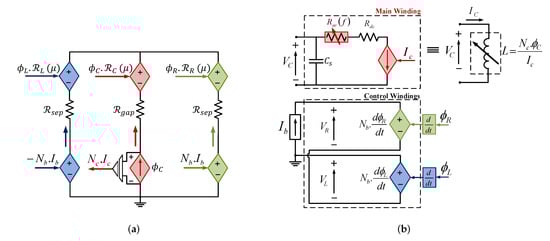
Figure 12.
Schematic of the variable inductor model based on the reluctance circuit. (a) Magnetic circuit, and (b) electric circuit.
On the other hand, Figure 12b illustrates the electrical system, which includes the electrical model of the winding, as well as the input voltage and the output current source. The electrical part of the three windings is represented by Equation (21).
where is the voltage at winding w, is the magnetic flux created by the winding w, and is the number of turns of the winding w. The winding w refers to the left (L), right (R), or center (C) windings. In order to account for the main winding DC losses, a constant resistor, , is added to the electrical circuit of the main winding in series with the current-controlled current source, which represents the main winding current. Also, to represent the AC winding losses, a variable frequency-dependent resistor, , is added in series to .
6. Model Validation Using Simulations and Experimental Results
In order to compare the initial lossless equivalent circuit with the proposed model, which includes core and winding losses, detailed simulations have been carried out. Furthermore, those two simulation models have been compared against experimental measurements obtained from the variable inductor prototype shown in Figure 13. The device has been developed based on the double E-core structure with the design specifications indicated in Table 5, and the models have been adjusted correspondingly.
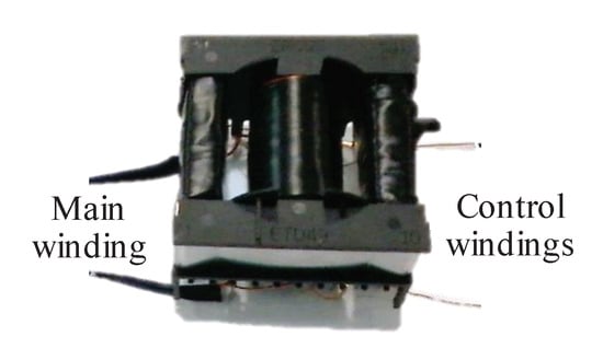
Figure 13.
Variable inductor prototype based on double the E-core structure.
Table 5.
Specifications of the test setup developed to validate the full VI model.
Figure 14a shows a circuit diagram of the developed test platform. It consists of a SiC full-bridge DC-AC converter to apply a square waveform excitation voltage on the inductor main winding. As mentioned previously, the square waveform voltage allows testing the device model under non-sinusoidal conditions, thus assure the validation of the loss study under a general condition of excitation voltage. The converter is controlled using a TMS320F28335 Texas Instruments peripheral board. Additionally, a variable DC voltage source is connected in series with a resistor to provide a DC control current of maximum 1 A to the control winding of the variable inductor. The constructed test platform is illustrated in Figure 14b.
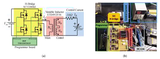
Figure 14.
Experimental setup used to test the variable inductor under small and large-signal analyses. (a) Circuit diagram, and (b) test platform.
6.1. Small-Signal Analysis
To validate the proposed model under small-signal analysis, the control current was increased from 0 to 1 A in steps of 0.05 A, while keeping zero excitation voltage on the main winding. The equivalent inductance seen from the main winding was measured using the impedance analyzer. Figure 15a illustrates the measurement of the equivalent inductance as a function of the bias control current. Also, the figure illustrates the simulated inductance obtained from the developed models, the initial lossless equivalent circuit, as well as the proposed model, which includes losses. Figure 15b shows the error of each model compared to the experimental results, as calculated by Equation (22). It can be observed that the proposed model that includes losses predicts the inductance within an acceptable error (<6%). On the other hand, the inductance predicted by the initial lossless model shows a clear deviation from the experimental one as the control current increases. It reaches an error of 30% at maximum control current.
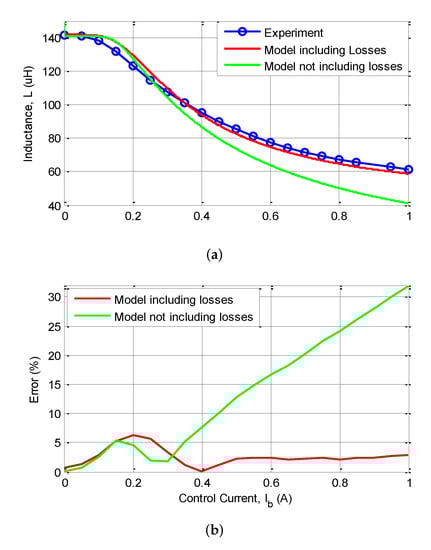
Figure 15.
Small-signal characterization of the variable inductor prototype comparing simulation models with experimental results. (a) Inductance value, and (b) percentage error as a function of control current.
6.2. Large-Signal Analysis
The prototype has also been characterized under large-signal analysis. Similar to the small-signal analysis, a DC control current is applied to the control windings and varied from 0 to 1 A. However, in this case, a square waveform voltage of 30 V is applied to the main winding of the inductor. The inductance is calculated by two different methods using the experimental measurements of the voltage and current through the main winding. The first method calculates the inductance using the RMS values of the waveforms over each cycle at a steady state. On the other hand, the second method uses the instantaneous values of the waveforms. The two methods were then compared to verify the accuracy of the measured inductance value, as explained hereafter.
6.2.1. Impedance Calculation
A simplification applied by considering the RMS value of the first harmonic component of the voltage and current measurements, so the resulting inductance is calculated by Equation (23).
where is the voltage applied to the main winding of the variable inductor, and is the current flowing through it.
6.2.2. System Identification Tools
The System Identification Toolbox from Matlab® is used, which requires a set of data that represent the input and output variables of a system; in this case, is the input to the system, and is the output. Using these variables, the tool defines the transfer function of the system based on the user selection of the number of poles and zeros of the system. In the case of an inductor, the system is defined as a 1st order system (1 pole, no zeros), and the transfer function is stated by Equation (24).
Figure 16 compares both methods of inductance calculation to verify the accuracy of the measured inductance and then uses it to assess the proposed model. It shows that the inductance calculated based on RMS values is in very close agreement with the inductance obtained by the Matlab® identification tool. This conclusion justifies the use of RMS measurements for calculating the inductance in the large-signal analysis in order to simplify the computations.
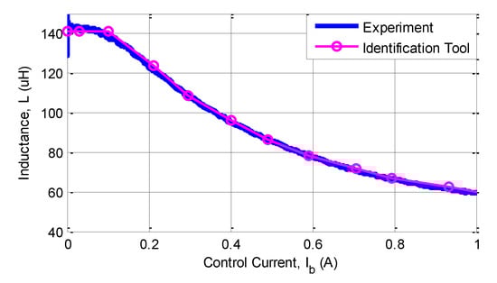
Figure 16.
Inductance calculation from experimental measurement.
Similar to the previous small-signal analysis, Figure 17a illustrates the equivalent inductance as a function of the bias control current for the large-signal analysis case. Figure 17b clarifies the trend of deviation or convergence of the models as a function of the control current, compared to the measured results. The results are quite consistent with the previous small-signal analysis; the inductance calculated by the proposed model still approaches the experimental measurements, while the one calculated by the lossless model shows a clear dispersion.
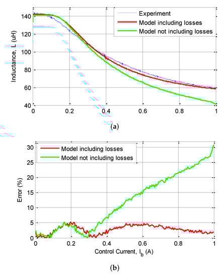
Figure 17.
Large-signal characterization of the variable inductor prototype comparing simulation models with experimental results. (a) Inductance value, and (b) percentage error as a function of control current.
7. Conclusions and Future Developments
In this paper, a full accurate circuit-based time-domain model for a variable magnetic device has been developed, demonstrated, and experimentally validated. The model can predict the inductance variation as a function of the control current in a variable magnetic element. The main contribution of this work is the development of a model that can be used in several simulation platforms, and, moreover, the inclusion of core losses as well as winding eddy current losses in the magnetic device. Additionally, it solves the causality issues, which are present in previous approaches.
A double E-core variable inductor prototype has been characterized under small-signal as well as large-signal analyses in order to assess the accuracy of the model. The proposed approach is considered an autonomous tool that can analyze any given set of data (simulated or experimental) for a magnetic core, detect the operation frequency, and correspondingly, adjust the magnetic core model with the core and winding loss parameters, and finally predict the inductance as a function of the control current, along with other electric and magnetic quantities that characterize the magnetic core operation. Consequently, only one simulator environment is used for the design and simulation of the electromagnetic system.
The test results validate the model under operation frequencies of hundreds of kHz (<200 kHz). Accordingly, the future developments of this work include the extension of the model’s validity to frequency ranges of 1–1.5 MHz. Also, the employment of the developed electromagnetic model to study the behavior of the variable inductor in a power electronic converter, specifically a DAB converter. The proposed model will allow for several studies using time-domain simulations, such as the control of the converter power transfer using the variable inductor, the possibility of the linearization of the system transfer function, and finally, the boost of the efficiency over critical operation ranges, for example, light load and heavy load operation ranges.
Author Contributions
S.S. and J.G. conceived the research and designed and performed the experiments; R.G. contributed to the reviewing and editing; all the authors analyzed the data and contributed in the discussion and conclusions. All authors have read and agreed to the published version of the manuscript.
Funding
This work has been partially supported by the Spanish Government, Innovation Development, and Research Office (MEC), under research grant ENE2016-77919, Project “Conciliator”, and by the European Union through ERFD Structural Funds (FEDER). Also, this work has been partially supported by the government of Principality of Asturias, Foundation for the Promotion in Asturias of Applied Scientific Research and Technology (FICYT), under Grant FC-GRUPIN-IDI/2018/000241 and under Severo Ochoa research grants, PA-13-PF-BP13-138 and PF-BP16-133.
Conflicts of Interest
The authors declare no conflict of interest. The founding sponsors had no role in the design of the study; in the collection, analyses, or interpretation of data; in the writing of the manuscript, and in the decision to publish the results.
Abbreviations
The following abbreviations are used in this manuscript:
| PEC | Power Electronic Converter |
| EMI | Electro-Magnetic Interference |
| DAB | Dual-Active-Bridge |
| FEA | Finite Elements Analysis |
| JA | Jiles-Atherton |
| FFT | Fast Fourier Transform |
References
- Fan, H.; Li, H. High-Frequency Transformer Isolated Bidirectional DC–DC Converter Modules With High Efficiency Over Wide Load Range for 20 kVA Solid-State Transformer. IEEE Trans. Power Electron. 2011, 26, 3599–3608. [Google Scholar] [CrossRef]
- Burgio, A.; Menniti, D.; Motta, M.; Pinnarelli, A.; Sorrentino, N.; Vizza, P. A laboratory model of a dual active bridge DC-DC converter for a smart user network. In Proceedings of the 2015 IEEE 15th International Conference on Environment and Electrical Engineering (EEEIC), Rome, Italy, 10–13 June 2015. [Google Scholar]
- Saeed, S.; Garcia, J. Extended Operational Range of Dual-Active-Bridge Converters by using Variable Magnetic Devices. In Proceedings of the 2019 IEEE Applied Power Electronics Conference and Exposition (APEC), Anaheim, CA, USA, 17–21 March 2019; pp. 1629–1634. [Google Scholar]
- Takach, M.; Lauritzen, P. Survey of magnetic core models. In Proceedings of the 1995 IEEE Applied Power Electronics Conference and Exposition, Dallas, TX, USA, 5–9 March 1995. [Google Scholar]
- Chen, Q.; Xu, L.; Ruan, X.; Wong, S.C.; Tse, C.K. Research and Development on New Control Techniques for Electronic Ballasts Based on Magnetic Regulators. Ph.D. Thesis, Dept. Elect. Comput. Eng., Univ. Coimbra, Coimbra, Portugal, 2012. [Google Scholar]
- Chen, Q.; Xu, L.; Ruan, X.; Wong, S.C.; Tse, C.K. Gyrator-Capacitor Simulation Model of Nonlinear Magnetic Core. In Proceedings of the 2009 Twenty-Fourth Annual IEEE Applied Power Electronics Conference and Exposition, Washington, DC, USA, 15–19 February 2009. [Google Scholar]
- Ludwig, G.; El-Hamamsy, S.A. Coupled inductance and reluctance models of magnetic components. IEEE Trans. Power Electron. 1991, 6, 240–250. [Google Scholar] [CrossRef]
- Almaguer, J.; Cárdenas, V.; Espinoza, J.; Aganza-Torres, A.; González, M. Performance and Control Strategy of Real-Time Simulation of a Three-Phase Solid-State Transformer. Appl. Sci. 2019, 9, 789. [Google Scholar] [CrossRef]
- Alonso, J.M.; Martinez, G.; Perdigao, M.; Cosetin, M.; do Prado, R.N. Modeling magnetic devices using SPICE: Application to variable inductors. In Proceedings of the 2016 IEEE Applied Power Electronics Conference and Exposition (APEC), Long Beach, CA, USA, 20–24 March 2016. [Google Scholar]
- Mandache, L.; Topan, D.; Sirbu, I.G. Accurate Time-Domain Simulation of Nonlinear Inductors Including Hysteresis and Eddy-Current Effects. In Proceedings of the World Congress on Engineering, London, UK, 6–8 July 2011; Volume 2. [Google Scholar]
- LTspice® Design Center. Available online: https://www.analog.com/en/design-center/design-tools-and-calculators/ltspice-simulator.html (accessed on 10 April 2020).
- MathWorks Simulink® Documentation. Available online: https://es.mathworks.com/help/simulink/index.html?s_cid=doc_ftr (accessed on 10 April 2020).
- PSIM User’s Guide. Available online: https://www.myway.co.jp/products/psim/dlfiles/pdf/PSIM_User_Manual_V9.0.2.pdf (accessed on 10 April 2020).
- Medini, D.; Ben-Yaakov, S. A current-controlled variable-inductor for high frequency resonant power circuits. In Proceedings of the 1994 IEEE Applied Power Electronics Conference and Exposition, Orlando, FL, USA, 13–17 February 1994. [Google Scholar]
- Sun, J. Recent Development in Ferrite Material for High Power Application [Passive Components]. IEEE Power Electron. Mag. 2018, 5, 21–25. [Google Scholar] [CrossRef]
- Brauer, J. Simple equations for the magnetization and reluctivity curves of steel. IEEE Trans. Magn. 1975, 11, 81. [Google Scholar] [CrossRef]
- Johansson, P.; Andersson, B. Comparison of Simulation Programs for Supercapacitor Modelling. Master’s Thesis, Chalmers University of Technology, Gothenburg, Sweden, 2008. Available online: http://webfiles.portal.chalmers.se/et/MSc/AnderssonJohanssonMSc.pdf (accessed on 10 April 2020).
- Saeed, S.; Garcia, J.; Georgious, R. Modeling of variable magnetic elements including hysteresis and Eddy current losses. In Proceedings of the 2018 IEEE Applied Power Electronics Conference and Exposition (APEC), San Antonio, TX, USA, 4–8 March 2018. [Google Scholar]
- Cardelli, E.; Fiorucci, L.; Torre, E.D. Estimation of MnZn ferrite core losses in magnetic components at high frequency. IEEE Trans. Magn. 2001, 37, 2366–2368. [Google Scholar] [CrossRef]
- Reinert, J.; Brockmeyer, A.; Doncker, R.D. Calculation of losses in ferro- and ferrimagnetic materials based on the modified Steinmetz equation. IEEE Trans. Ind. Appl. 2001, 37, 1055–1061. [Google Scholar] [CrossRef]
- Jiles, D.; Atherton, D. Ferromagnetic hysteresis. IEEE Trans. Magn. 1983, 19, 2183–2185. [Google Scholar] [CrossRef]
- Wilson, P.R. Modelling and Simulation of Magnetic Components in Electric Circuits. Ph.D. Thesis, School of Electronics and Computer Science, University of Southampton, Southampton, UK, 2001. Available online: https://eprints.soton.ac.uk/368484/ (accessed on 10 April 2020).
- Ramesh, A.; Jiles, D.; Roderick, J. A model of anisotropic anhysteretic magnetization. IEEE Trans. Magn. 1996, 32, 4234–4236. [Google Scholar] [CrossRef]
- Pop, N.; Caltun, O. Jiles-Atherton Magnetic Hysteresis Parameters Identification. Acta Phys. Pol. A 2011, 120. Available online: http://przyrbwn.icm.edu.pl/APP/PDF/120/a120z3p22.pdf (accessed on 10 April 2020). [CrossRef]
- Xiao, C.; Chen, G.; Odendaal, W.G.H. Overview of Power Loss Measurement Techniques in Power Electronics Systems. IEEE Trans. Ind. Appl. 2007, 43, 657–664. [Google Scholar] [CrossRef]
- Thottuvelil, V.; Wilson, T.; Owen, H. High-frequency measurement techniques for magnetic cores. IEEE Trans. Power Electron. 1990, 5, 41–53. [Google Scholar] [CrossRef]
- Mu, M.; Li, Q.; Gilham, D.J.; Lee, F.C.; Ngo, K.D.T. New Core Loss Measurement Method for High-Frequency Magnetic Materials. IEEE Trans. Power Electron. 2014, 29, 4374–4381. [Google Scholar] [CrossRef]
- Dowell, P. Effects of eddy currents in transformer windings. Proc. Inst. Electr. Eng. 1966, 113, 1387. [Google Scholar] [CrossRef]
- Yin, Y.; Li, L. Improved method to calculate the high-frequency eddy currents distribution and loss in windings composed of round conductors. IET Power Electron. 2017, 10, 1494–1503. [Google Scholar] [CrossRef]
- Holguin, F.A.; Asensi, R.; Prieto, R.; Cobos, J.A. Simple analytical approach for the calculation of winding resistance in gapped magnetic components. In Proceedings of the 2014 IEEE Applied Power Electronics Conference and Exposition, Fort Worth, TX, USA, 16–20 March 2014. [Google Scholar]
- Massarini, A.; Kazimierczuk, M. Self-capacitance of inductors. IEEE Trans. Power Electron. 1997, 12, 671–676. [Google Scholar] [CrossRef]


© 2020 by the authors. Licensee MDPI, Basel, Switzerland. This article is an open access article distributed under the terms and conditions of the Creative Commons Attribution (CC BY) license (http://creativecommons.org/licenses/by/4.0/).