An Experimental Study on the Actuator Line Method with Anisotropic Regularization Kernel


Abstract
1. Introduction
2. Method
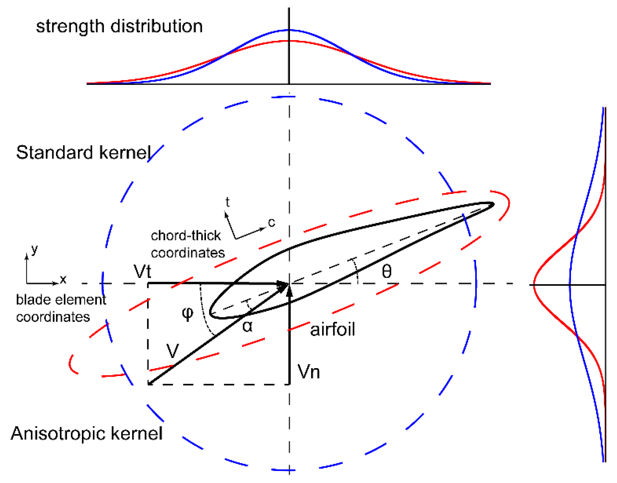
2.1. Actuator Line Method (ALM)
2.2. Tip Loss Correction
2.3. Simulation Setup
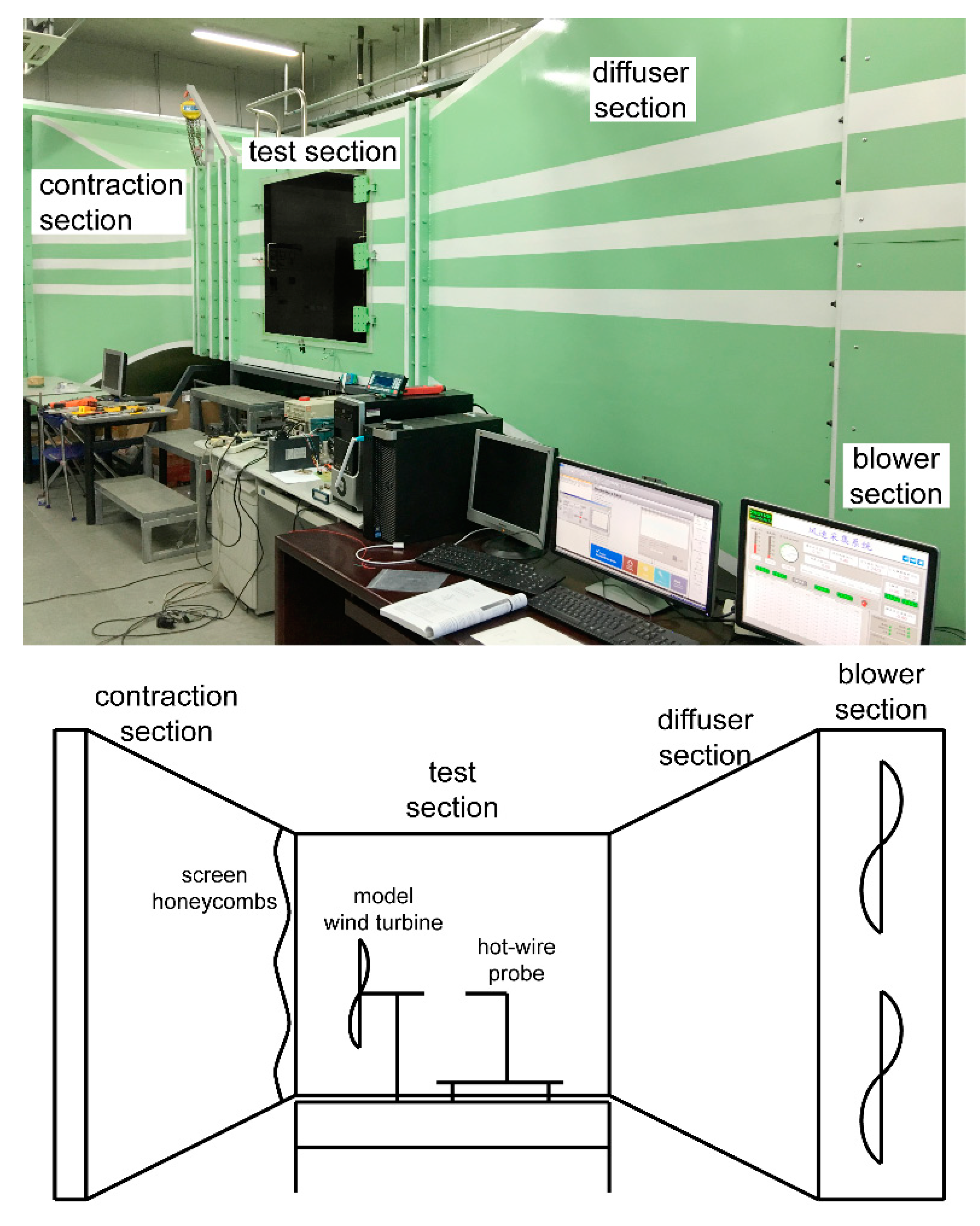
2.4. Experimental Setup
2.5. Frozen Rotor Method
3. Result
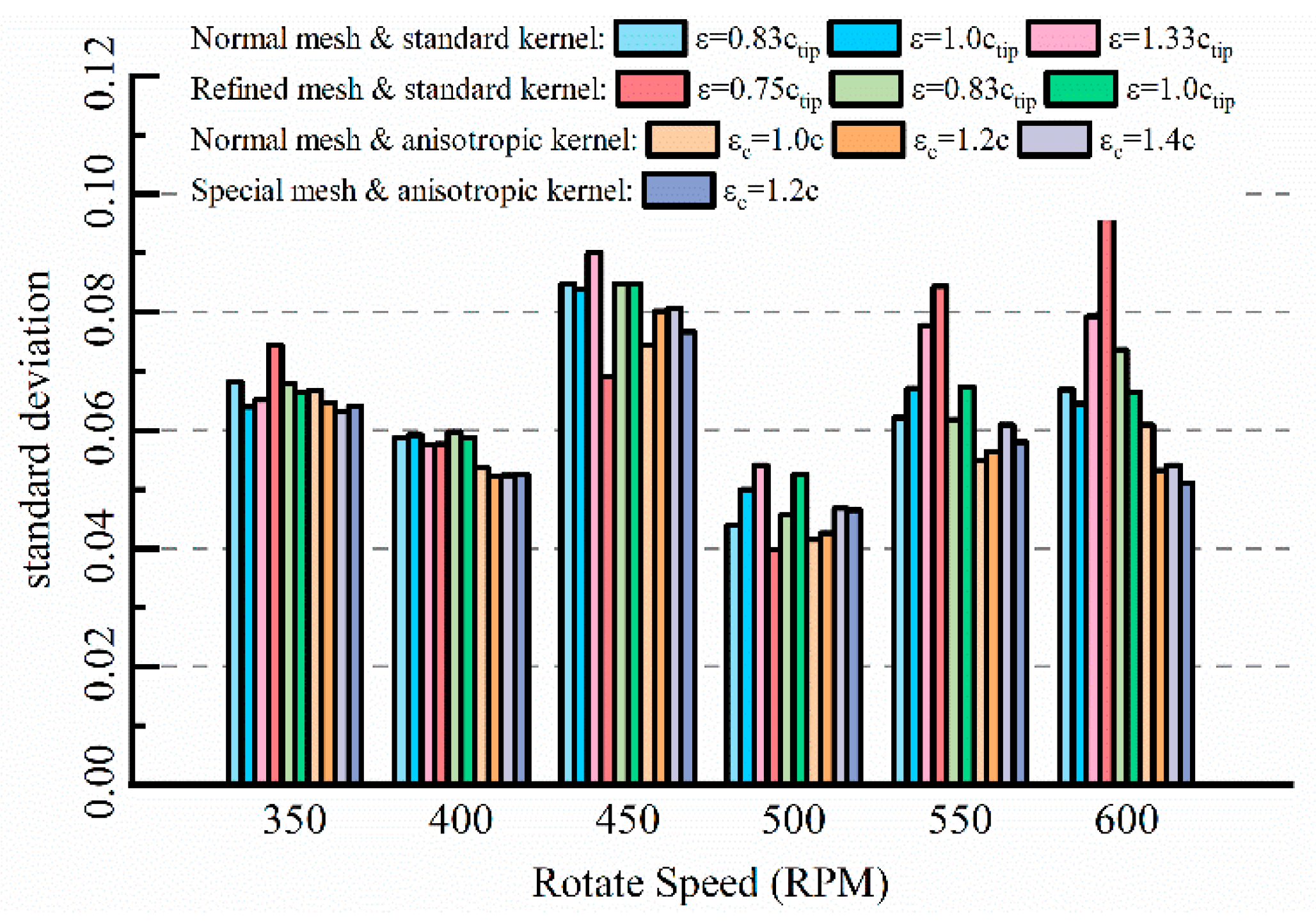
3.1. Mesh Independence
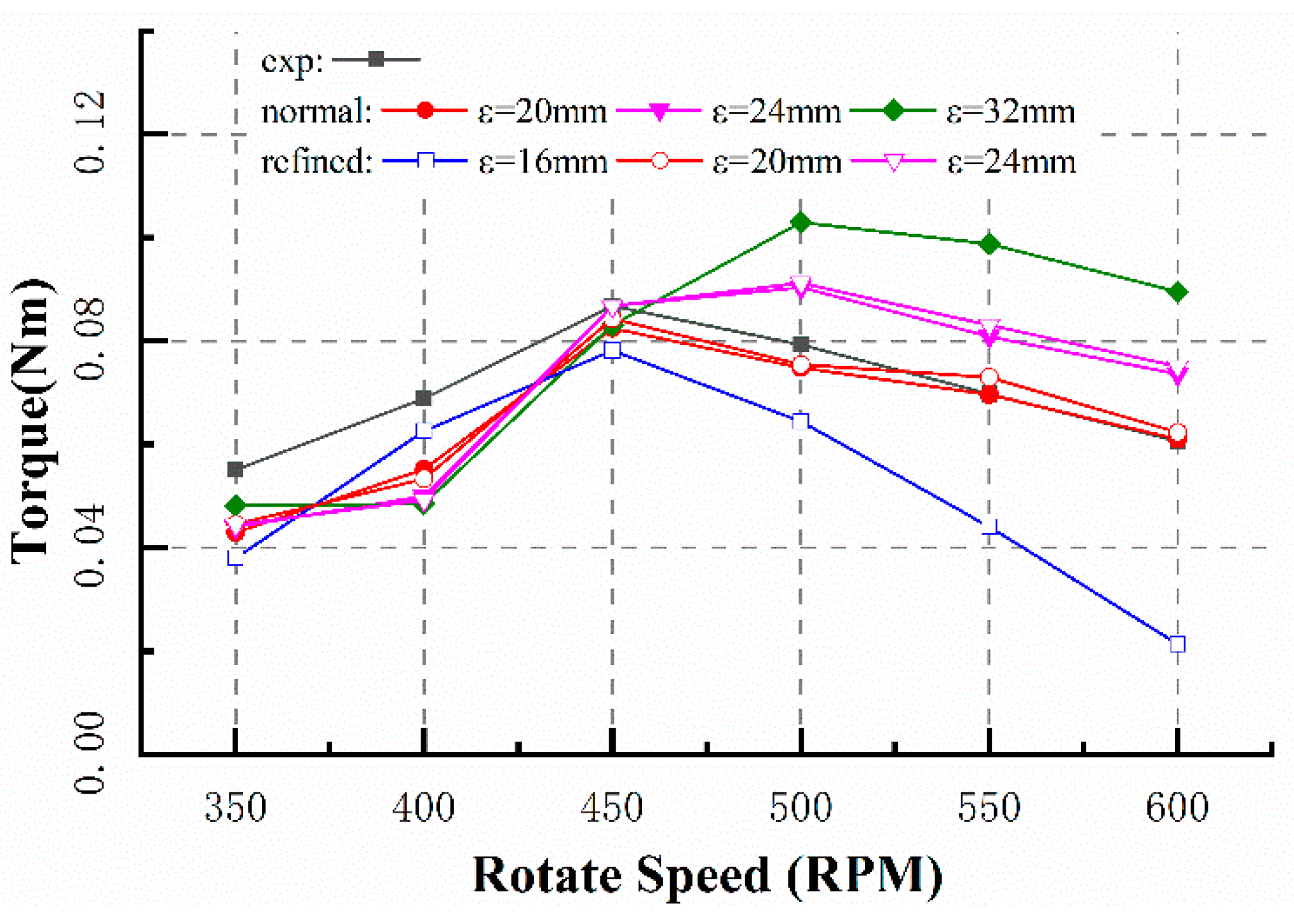
3.2. The Effect of Gaussian Width
3.3. The Effect of the Chord Length Gaussian Width
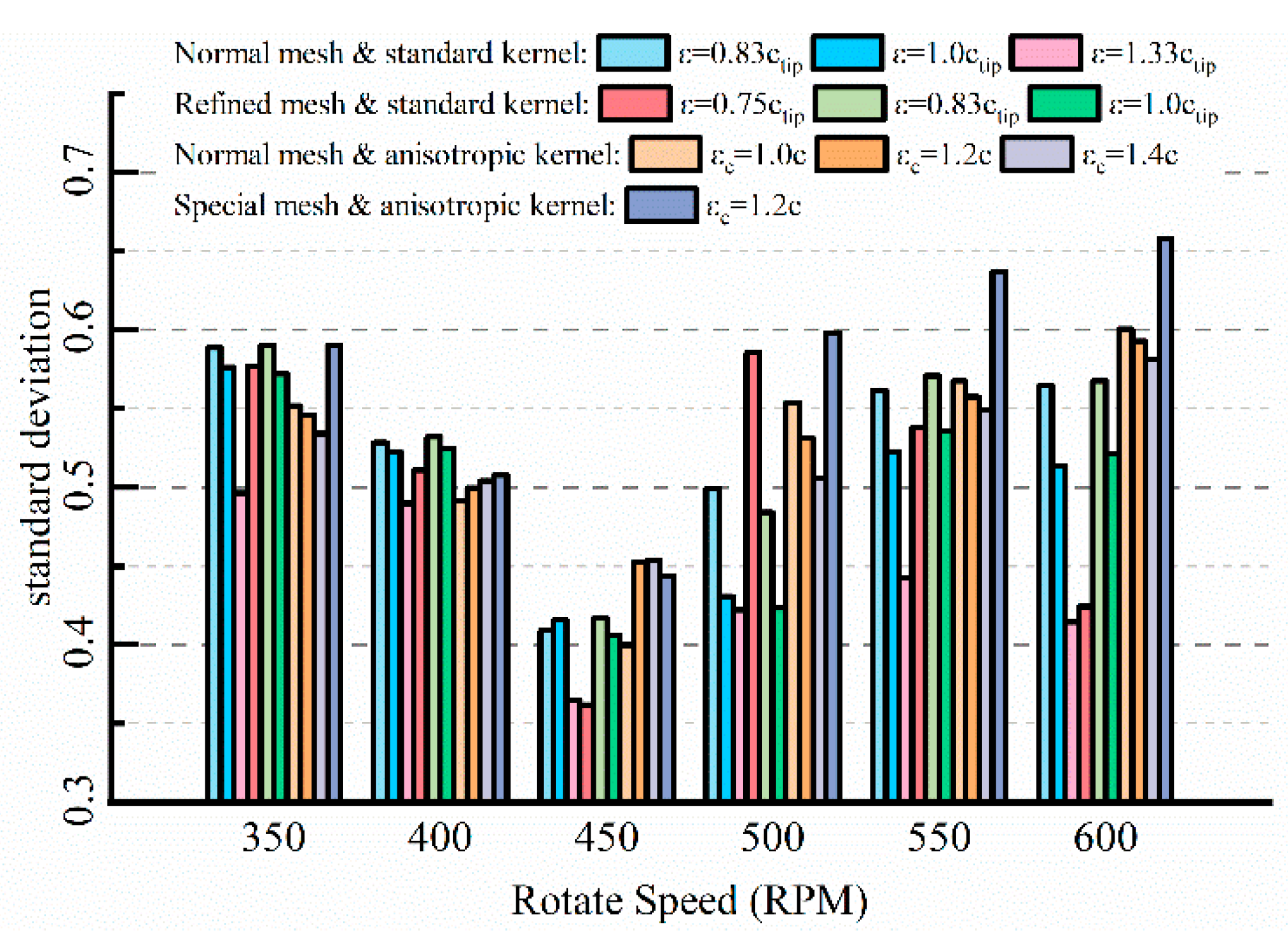
3.4. The Effect of the Thickness Gaussian Width
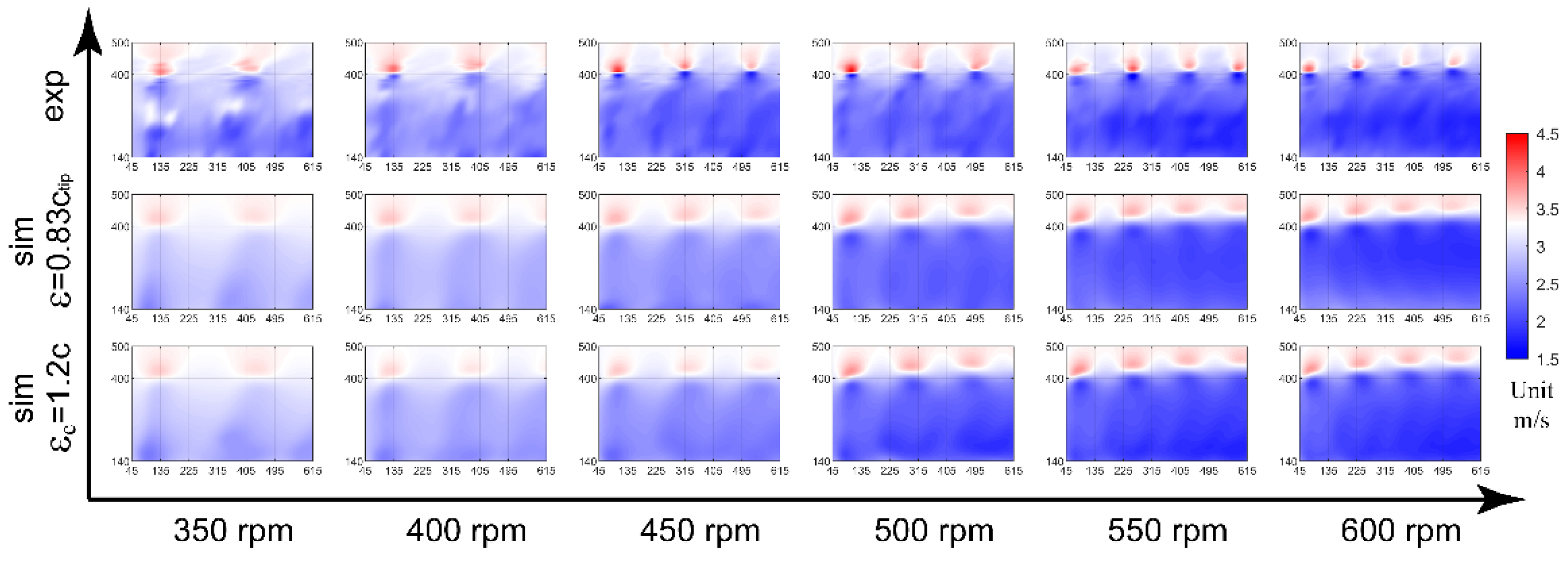
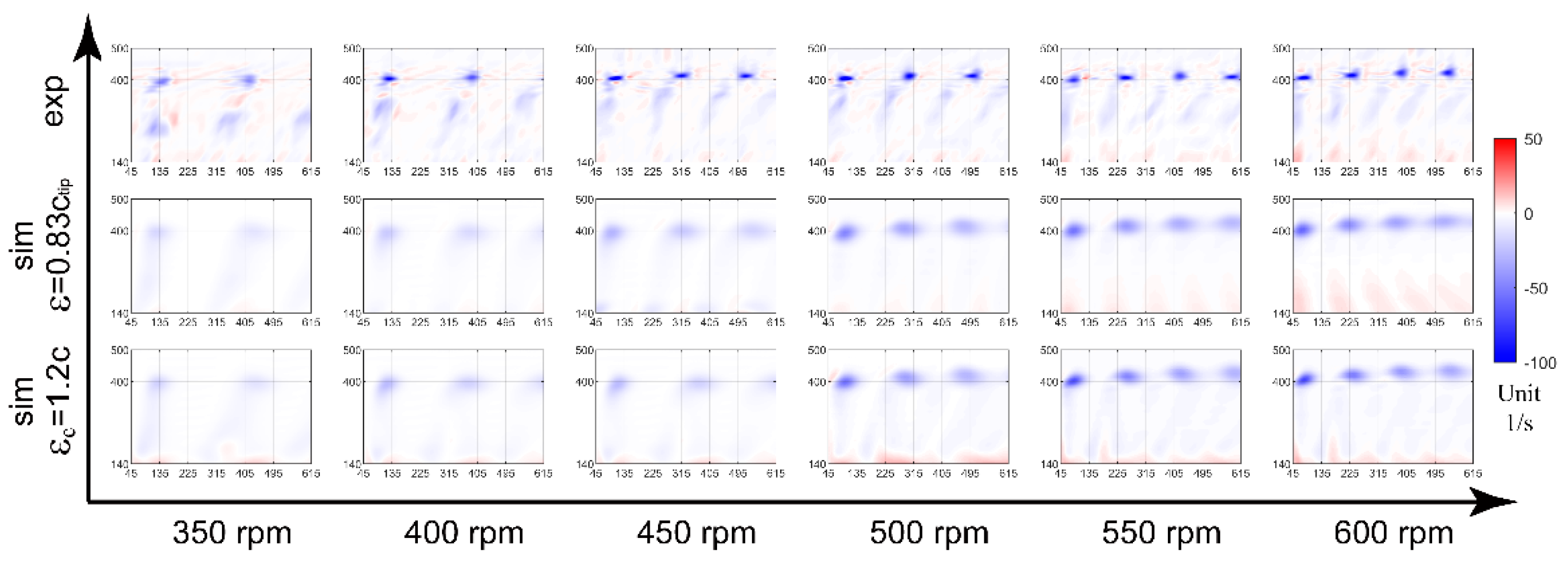
3.5. Wake Characteristic
4. Conclusions
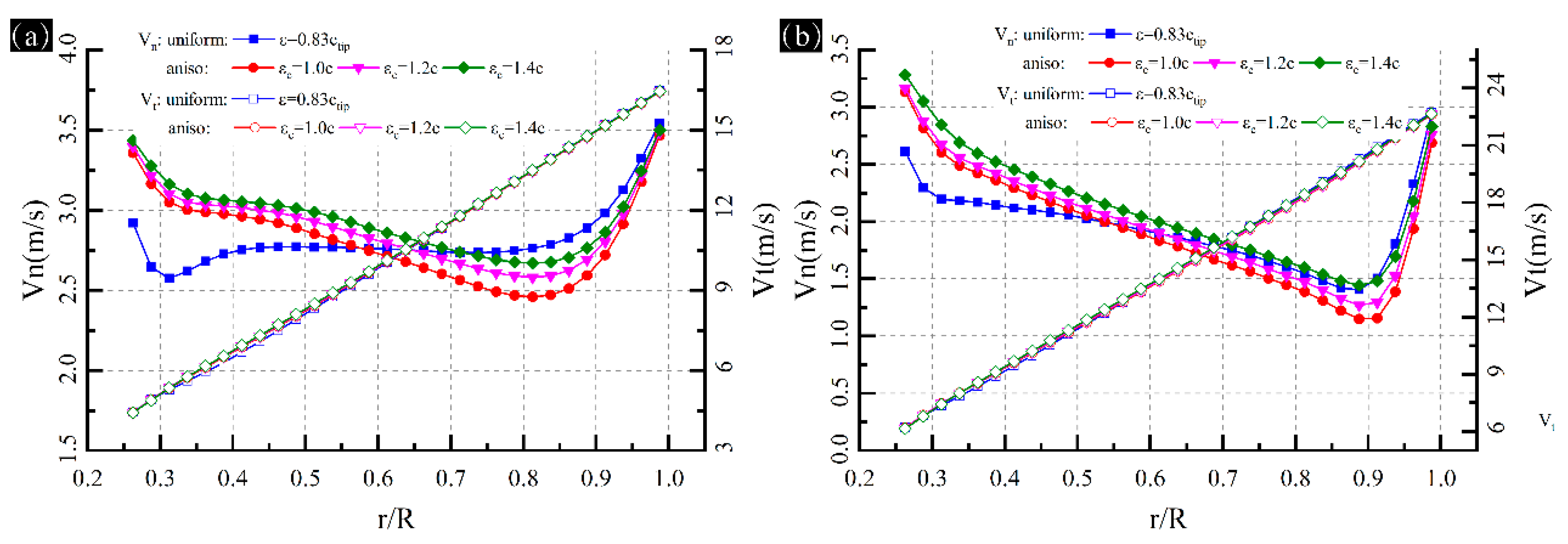
- Gaussian width will strongly affect the torque result during actuator line simulations and it does not converge when becomes larger. Larger ϵ value will cause a higher prediction of the normal velocity of each blade element, but has little effect on the tangential velocity. The influence of the value on the attack angle is the main reason for its effect on the torque prediction.
- In this study, for standard regularization kernel and for anisotropic kernel can guarantee a reliable torque result. However, according to the state-of-art studies, the optimal value for varies with the scale of wind turbine. It can be inferred that the suitable parameters are related to the Reynolds number.
- The thickness parameter has little influence on the torque prediction. However, the thickness parameter significantly affects the prediction of the wake characteristics. The anisotropic regularization kernel will improve the performance of the actuator line model in wake simulations.
- Borrowing the idea of frozen rotor method, this study developed a reliable method to measure the wind turbine wakes. The wake characteristics were reconstructed by simultaneously gathered velocity data and rotor azimuth.
- A special mesh with refinement in the main flow direction will take advantages of the anisotropic regularization kernel. Using a mesh refined in the main flow direction, ALM with anisotropic kernel can predict torque and wake characteristics better while maintaining low computational costs.
Author Contributions
Funding
Conflicts of Interest
Nomenclature
| Variables | |
| number of wind turbine blades | |
| free stream velocity [m/s] | |
| rotor speed [rad/s] | |
| rotor radius [m] | |
| radial position of th blade element | |
| inflow angle for th blade element | |
| regularization kernel | |
| Gaussian width for standard regularization kernel [m] | |
| chord length Gaussian width for anisotropic regularization kernel [m] | |
| thickness Gaussian width for anisotropic regularization kernel [m] | |
| length Gaussian width for anisotropic regularization kernel [m] | |
| air density [kg/m3] | |
| lift force [N] | |
| drag force [N] | |
| chord length [m] | |
| length of blade element [m] | |
| local velocity on blade element [m/s] | |
| lift coefficient | |
| drag coefficient | |
| distance from the center of regularization kernel [m] | |
| projection of on the chord length direction of blade element [m] | |
| projection of on the thickness direction of blade element [m] | |
| projection of on the length direction of blade element [m] | |
| standard deviation | |
| correlation coefficient | |
References
- Sorensen, J.N.; Shen, W.Z. Numerical modeling of wind turbine wakes. J. Fluid. Eng.-Trans. ASME 2002, 124, 393–399. [Google Scholar] [CrossRef]
- Martinez-Tossas, L.A.; Churchfield, M.J.; Leonardi, S. Large eddy simulations of the flow past wind turbines: Actuator line and disk modeling. Wind Energy 2015, 18, 1047–1060. [Google Scholar] [CrossRef]
- Mikkelsen, R.; Sørensen, J.N.; Øye, S.; Troldborg, N. Analysis of power enhancement for a row of wind turbines using the actuator line technique. J. Phys. Conf. Ser. 2007, 75, 012044. [Google Scholar] [CrossRef]
- Lee, S.; Churchfield, M.J.; Moriarty, P.J.; Jonkman, J.; Michalakes, J. A Numerical Study of Atmospheric and Wake Turbulence Impacts on Wind Turbine Fatigue Loadings. J. Solar Energy Eng.-Trans. ASME 2013, 135. [Google Scholar] [CrossRef]
- Storey, R.C.; Cater, J.E.; Norris, S.E. Large eddy simulation of turbine loading and performance in a wind farm. Renew. Energy 2016, 95, 31–42. [Google Scholar] [CrossRef]
- Na, J.S.; Koo, E.; Munoz-Esparza, D.; Jin, E.K.; Linn, R.; Lee, J.S. Turbulent kinetics of a large wind farm and their impact in the neutral boundary layer. Energy 2016, 95, 79–90. [Google Scholar] [CrossRef]
- Na, J.S.; Koo, E.; Jin, E.K.; Linn, R.; Ko, S.C.; Muñoz-Esparza, D.; Lee, J.S. Large-eddy simulations of wind-farm wake characteristics associated with a low-level jet. Wind Energy 2018, 21, 163–173. [Google Scholar] [CrossRef]
- Zhong, H.M.; Du, P.G.; Tang, F.N.; Wang, L. Lagrangian dynamic large-eddy simulation of wind turbine near wakes combined with an actuator line method. Appl. Energy 2015, 144, 224–233. [Google Scholar] [CrossRef]
- Ma, Z.; Zeng, P.; Lei, L.P. Analysis of the coupled aeroelastic wake behavior of wind turbine. J. Fluids Struct. 2019, 84, 466–484. [Google Scholar] [CrossRef]
- Meng, H.; Lien, F.S.; Li, L. Elastic actuator line modelling for wake-induced fatigue analysis of horizontal axis wind turbine blade. Renew. Energy 2018, 116, 423–437. [Google Scholar] [CrossRef]
- Sorensen, J.N.; Mikkelsen, R.F.; Henningson, D.S.; Ivanell, S.; Sarmast, S.; Andersen, S.J. Simulation of wind turbine wakes using the actuator line technique. Philos. Trans. A Math. Phys. Eng. Sci. 2015, 373, 20140071. [Google Scholar] [CrossRef] [PubMed]
- Martinez-Tossas, L.A.; Churchfield, M.J.; Meneveau, C. Optimal smoothing length scale for actuator line models of wind turbine blades based on Gaussian body force distribution. Wind Energy 2017, 20, 1083–1096. [Google Scholar] [CrossRef]
- Churchfield, M.J.; Schreck, S.J.; Martinez, L.A.; Meneveau, C.; Spalart, P.R. An advanced actuator line method for wind energy applications and beyond. In Proceedings of the 35th Wind Energy Symposium, Grapevine, TX, USA, 9–13 January 2017; p. 1998. [Google Scholar]
- Jha, P.K.; Churchfield, M.J.; Moriarty, P.J.; Schmitz, S. Guidelines for Volume Force Distributions Within Actuator Line Modeling of Wind Turbines on Large-Eddy Simulation-Type Grids. J. Solar Energy Eng.-Trans. ASME 2014, 136. [Google Scholar] [CrossRef]
- Troldborg, N. Actuator Line Modeling of Wind Turbine Wakes. Doctoral Thesis, Technical University of Denmark, Lyngby, Denmark, 2009. [Google Scholar]
- Troldborg, N.; Sorensen, J.N.; Mikkelsen, R.; Sorensen, N.N. A simple atmospheric boundary layer model applied to large eddy simulations of wind turbine wakes. Wind Energy 2014, 17, 657–669. [Google Scholar] [CrossRef]
- Shives, M.; Crawford, C. Mesh and load distribution requirements for actuator line CFD simulations. Wind Energy 2013, 16, 1183–1196. [Google Scholar] [CrossRef]
- Wu, Y.T.; Porte-Agel, F. Large-Eddy Simulation of Wind-Turbine Wakes: Evaluation of Turbine Parametrisations. Bound.-Layer Meteorol. 2011, 138, 345–366. [Google Scholar] [CrossRef]
- Shen, W.Z.; Sørensen, J.N.; Mikkelsen, R. Tip Loss Correction for Actuator/Navier–Stokes Computations. J. Solar Energy Eng. 2005, 127, 209–213. [Google Scholar] [CrossRef]
- Snel, H.; Schepers, J.; Montgomerie, B. The MEXICO project (Model Experiments in Controlled Conditions): The database and first results of data processing and interpretation. J. Phys. Conf. Ser. 2007, 75, 012014. [Google Scholar] [CrossRef]
- Hong, J.; Guala, M.; Chamorro, L.; Sotiropoulos, F. Probing wind-turbine/atmosphere interactions at utility scale: Novel insights from the EOLOS wind energy research station. J. Phys. Conf. Ser. 2014, 524, 012001. [Google Scholar] [CrossRef]
- Hong, J.; Toloui, M.; Chamorro, L.P.; Guala, M.; Howard, K.; Riley, S.; Tucker, J.; Sotiropoulos, F. Natural snowfall reveals large-scale flow structures in the wake of a 2.5-MW wind turbine. Nat. Commun. 2014, 5, 4216. [Google Scholar] [CrossRef]
- Hu, H.; Wei, T.; Wang, Z. An Experimental Study on the Wake Characteristics of Dual-Rotor Wind Turbines by Using a Stereoscopic PIV Technique. In Proceedings of the 34th AIAA Applied Aerodynamics Conference, Washington, DC, USA, 13–17 June 2016; p. 3128. [Google Scholar]
- Wang, Z.Y.; Ozbay, A.; Tian, W.; Hu, H. An experimental study on the aerodynamic performances and wake characteristics of an innovative dual-rotor wind turbine. Energy 2018, 147, 94–109. [Google Scholar] [CrossRef]
- Schumann, H.; Pierella, F.; Saetran, L. Experimental investigation of wind turbine wakes in the wind tunnel. Energy Procedia 2013, 35, 285–296. [Google Scholar] [CrossRef]
- Iungo, G.V.; Viola, F.; Camarri, S.; Porte-Agel, F.; Gallaire, F. Linear stability analysis of wind turbine wakes performed on wind tunnel measurements. J. Fluid Mech. 2013, 737, 499–526. [Google Scholar] [CrossRef]
- Singh, A.; Howard, K.B.; Guala, M. On the homogenization of turbulent flow structures in the wake of a model wind turbine. Phys. Fluids 2014, 26, 025103. [Google Scholar] [CrossRef]
- Dou, B.Z.; Guala, M.; Lei, L.; Zeng, P. Experimental investigation of the performance and wake effect of a small-scale wind turbine in a wind tunnel. Energy 2019, 166, 819–833. [Google Scholar] [CrossRef]
- Anik, E.; Abdulrahim, A.; Ostovan, Y.; Mercan, B.; Uzol, O. Active control of the tip vortex: An experimental investigation on the performance characteristics of a model turbine. J. Phys. Conf. Ser. 2014, 524, 012098. [Google Scholar] [CrossRef]
- Sarlak, H.; Mikkelsen, R.; Sarmast, S.; Sørensen, J.N. Aerodynamic behaviour of NREL S826 airfoil at Re= 100,000. J. Phys. Conf. Ser. 2014, 524, 012027. [Google Scholar] [CrossRef]


| Region | Background | Rotor and Wake | Total Number | Element Size (Rotor and Wake) | |
|---|---|---|---|---|---|
| Mesh Level | |||||
| Normal | 228,608 | 800,000 | 1,112,108 | 10 mm, uniform | |
| Refined | 228,608 | 1,562,500 | 1,903,858 | 8 mm, uniform | |
| Special | 228,608 | 1,340,000 | 1,673,708 | 10 mm in rotor plane 6 mm in main flow direction | |
| Speed | Exp | ||
|---|---|---|---|
| 350 | 0.05504 | 0.04202 | 0.04291 |
| 400 | 0.06889 | 0.06014 | 0.05979 |
| 450 | 0.08679 | 0.08384 | 0.07998 |
| 500 | 0.07922 | 0.07701 | 0.07870 |
| 550 | 0.0697 | 0.07000 | 0.06982 |
| 600 | 0.06062 | 0.06228 | 0.06105 |
© 2020 by the authors. Licensee MDPI, Basel, Switzerland. This article is an open access article distributed under the terms and conditions of the Creative Commons Attribution (CC BY) license (http://creativecommons.org/licenses/by/4.0/).
Share and Cite
Ma, Z.; Lei, L.; Dowell, E.; Zeng, P. An Experimental Study on the Actuator Line Method with Anisotropic Regularization Kernel. Energies 2020, 13, 977. https://doi.org/10.3390/en13040977
Ma Z, Lei L, Dowell E, Zeng P. An Experimental Study on the Actuator Line Method with Anisotropic Regularization Kernel. Energies. 2020; 13(4):977. https://doi.org/10.3390/en13040977
Chicago/Turabian StyleMa, Zhe, Liping Lei, Earl Dowell, and Pan Zeng. 2020. "An Experimental Study on the Actuator Line Method with Anisotropic Regularization Kernel" Energies 13, no. 4: 977. https://doi.org/10.3390/en13040977
APA StyleMa, Z., Lei, L., Dowell, E., & Zeng, P. (2020). An Experimental Study on the Actuator Line Method with Anisotropic Regularization Kernel. Energies, 13(4), 977. https://doi.org/10.3390/en13040977