Abstract
A mathematical model for the design of small-scale supply chains for liquefied natural gas (LNG) has been developed. It considers the maritime delivery of LNG from supply ports to satellite terminals and land-based transports from the terminals to consumers on or off the coast. Both tactical and strategic aspects in the supply chain design are addressed by optimizing the maritime routing of a heterogeneous fleet of ships, truck connections, and the locations of the satellite terminals. The objective is to minimize the overall cost, including operation and investment costs for the selected time horizon. The model is expressed as a mixed-integer linear programming problem, applying a multi-period formulation to determine optimal storage sizes and inventory at the satellite terminals. Two case studies illustrate the model, where optimal LNG supply chains for a region with sparsely distributed island (without land transports) and a coastal region at a gulf (with both sea and land transports) are designed. The model is demonstrated to be a flexible tool suited for the initial design and feasibility analysis of small-scale LNG supply chains.
1. Introduction
Natural gas can be liquefied at atmospheric pressure by cooling it below −162 °C, which increases the density by a factor of 600 and yields what is called liquefied natural gas (LNG). Since the liquefaction includes several purification steps, LNG represents a clean fossil fuel. As it primarily holds methane, its hydrogen-to-carbon ratio is high and the CO2 emissions are therefore clearly lower than for other fossil fuels. Due to these facts, LNG has gained considerable popularity recently, and it has been considered a key bridge fuel during a gradual transition in the world towards using energy sources with lower or no fossil CO2 emissions [1,2]. Other key drivers are the recently imposed regulations against pollution in maritime transportation, where the use of heavy fuel oil has been banned in certain emission control areas by the International Maritime Organization, and the need for gas very far from the gas sources or at stranded locations. LNG also plays a role in the strategic energy independence of certain regions. It has been estimated that 15% of the global gas use will be provided as LNG by 2040 [3]. However, the supply chain from wellhead to regasification of LNG is complex and comprises many steps [4]: because of the characteristics of LNG, including the low temperature and boil-off gas that must be handled, specific infrastructure is required for the transportation and storage. Networks for large-scale transportation of LNG over long distances (“liner shipping”) have already been available for decades, with typical tanker sizes of 150,000 m3. The design of such large-scale supply chains requires the consideration of many factors, including costs, flexibility, and energy security [5,6]. However, not until recently there has been a growing interest in small-scale LNG supply chains that could serve middle- to small-scale consumers in sparsely distributed areas. Such small-scale supply chains show many different features compared to the large-scale chains: the vessels have a capacity of 1000–40,000 m3, the shiploads may be split on consecutive receiving ports and the transportation distances are considerably shorter. Satellite terminals that receive LNG from the ships have smaller storage tanks (<50,000 m3) which are to be filled weekly or a few times a month. Because of the specific infrastructure (ships, storage, gas-handling equipment, etc.) and the moderate quantities delivered, the small-scale LNG chains are associated with high relative investment costs. This stresses the need for an optimal design of the supply chain.
The model developed in this paper is based on earlier work by the authors [7,8], where a single-period model was developed for the design of small-scale LNG supply chains. The formulation addresses both strategic and tactic decisions, where the location of the satellite terminals, the size of the fleet of vessels, and their routing and deliveries are optimized. It extends the earlier model to a multi-period optimization, where also the size of the storages and the inventory levels are considered, and simultaneous possible land transportation to off-cost regions. This complicates the problem considerably as the added options are combinatorial. This is a vehicle routing problem (VRP), which has been extensively studied in the literature (e.g., [9]), but some aspects considered here are not treated in classical VRPs but belong to other classes of sub-problems. The task of determining the number of vessels and their sizes is a fleet-size and mix-vehicle routing problem (FSMVRP) while the location of satellite terminals and the optimal ship routing to them is a location-routing problem (LRP). Finally, the sizing of storage tanks and the determination of the optimal inventory levels represent features of inventory routing problems (IRP). For a more detailed treatment of these type of general problems, the reader is referred to Hoff et al. [10], who summarizes FSMVRP with both maritime and land transport in a review paper, a survey and classification of LRP provided by Drexl and Schneider [11], as well as a review of IRP by Andersson et al. [12].
Most of the approaches of LNG supply chain optimization proposed in the literature focus on heuristics [13] or evolutionary solutions and very few papers present exact methods. Baldacci et al. [14] designed a mixed-integer linear programming (MILP) model for solving an FSMVRP problem similar to the one considered in the present paper, but where each customer was associated with a single route as in the classic VRP. By contrast, in our approach, we allow for multiple visits to customers by multiple ships. This feature also occurs in the formulation of the LRP sub-problem.
Most of the variables used for describing the activation of satellite terminals and their associated routes and delivery of the present paper are the same as those used in the literature (e.g., [15]), but the set of binary variables to activate the routes associated with an activated satellite terminal has been changed into integer variables to allow for multiple voyages to the same port. According to the classification in [12], the present approach falls into the finite time class, featuring deterministic demand, many-to-many topology, multiple routing, fixed inventory, and heterogeneous fleet composition. A contribution presenting similar features with a deterministic approach is the work by Al-Khayyal and Hwang [16] for an IRP for multi-commodity liquid bulk. Their problem is a classic IRP problem, where storage sizes are given as well as the fleet of ships and the model focuses on the key aspects of a multi-product pickup-delivery problem. A paper by Koza et al. [17] presents many characteristics similar to our problem, including the focus on the LNG market and infrastructure. Our contribution differs with respect to the market-segment (small-scale logistics versus liner networks), the locating of satellite terminals, and the multi-period formulation for optimized storage sizing and inventory. Furthermore, our approach is based on an arc-flow formulation while Koza et al. used a path-based model. Budiyanto et al. [18] present a capacitated vehicle routing problem for a small-scale LNG supply chain with fixed terminals, considering different options for the fleet of ships and pertinent constraints (e.g., imposed by port depth) but studied only two promising routes in detail.
In summary, the literature on routing problems often favors path-flow formulations over arc-based ones: with the feasible routes being predefined, the former formulation does not include constraints related to routing feasibility but focuses on the set of ports or customers to serve. Even with these simplifications, the solution time for exact methods becomes too long, so heuristic solution strategies have been preferred. By contrast, we apply an exact method but neglect some operational aspects that are not essential for initial planning of supply chains: we do not consider scheduling, supply availability according to production rate or inventory, boil-off loss, time windows at the ports, or load-dependent fuel consumption in the transportation vehicles. With these simplifications, a MILP model was formulated that can solve real problems within a few hours of computation time.
The model is illustrated by two case studies. First, it is applied to a problem with LNG supply to islands from one supply port, disregarding the option of land transportation. This example illustrates how the multi-period formulation can find better solutions than those of a single-period problem. The second example, where the full features of the model are utilized, studies an emerging LNG market in the Gulf of Bothnia that supplies LNG to Finland and Sweden. At the end of the paper, some conclusions concerning the applicability of the model are drawn and future potential directions of research in the field are proposed.
2. Problem Formulation
The task studied in this paper is a regional supply problem of LNG from a set of possible supply ports to end customers through a set of potential satellite terminals. LNG is loaded to specially designed ships at the supply ports and transported to the satellite terminals. It can also be transported by truck from the ports to inland customers. Land transportation by truck instead of by pipeline is economically justified for relatively scattered consumers with small energy demands. The satellite terminals are optional, but their locations are given, and they can be activated if beneficial for the overall objective. The sites of the potential satellite terminals and inland customers have given energy demands for the time horizon considered, which must be satisfied either by LNG or by an alternative fuel. This alternative fuel is used to make it possible to partly or fully exclude customers from the LNG supply chain: the transportation costs of the alternative fuel is not considered. The demand sites represent clusters of consumers, which justifies the use of multiple fuels. The fleet of ships can be freely chosen from a set of heterogeneous ship types, each with a given cruising speed, capacity, fuel consumption, and loading/unloading rate. The ships can perform split delivery and there are no limitations on routes or ship-port connections. The amount of LNG available at the supply ports is limited. LNG tank trucks for land-based transportation are of given capacity and fuel consumption and cannot perform split delivery. Each truck is associated with a single supply or satellite terminal, cannot be filled at other ports, and has a maximum traveling distance. The number of trucks is limited by the number of filling stations at the ports and the weekly working hours at the facilities. Inland customers have enough storage capacity to stock the full LNG demand for the time horizon and the investment costs in their tanks and other required facilities are disregarded. However, size-dependent investment costs for the storage tanks in the activated satellite terminals are considered. The optimization involves three key decisions: to locate the satellite terminals, to determine the fleet and routing for both maritime and land transportation, and to size the storage tanks at the satellite terminals and to determine their inventory levels.
3. Mathematical Model
In the multi-period problem with periods, each with a time horizon of , that is formulated, denotes the set of time periods indexed by , and are sets of satellite terminals and supply ports, respectively, while the set of all ports is . Let be the set of inland customers and the set of all customers of a given demand . The indexed set of ship types is . The arc set is defined as and represents all the sailing legs between port pairs. denotes the land-based port-consumer connection, with distances below . The maritime routing is defined by the three sets of variables: integer variables indicate how many times ship type travels the sailing leg , continuous variables specify the number of LNG loads transported by ship type on route , while the ship types represented in the fleet are given by binary variables . Likewise, three sets of variables describe the land-based transport: continuous variables express the quantity of LNG transported on the route , the number of allocated trucks per port and the number of trips per route are given by integer variables and , respectively, while binary decision variables activate satellite terminals. The continuous variables and represent the storage size of the activated satellite terminals and the inventory at the beginning of each time period, respectively. The supply of alternative fuel to the consumers is . All the symbols are defined in the Nomenclature at the end of the paper.
The objective of the problem is to minimize the combined fuel, operation, and investment costs
The first term expresses the cost of LNG transported by ship as a product of the LNG price, the ship capacity, and the number of LNG loads transported. The second term holds the cost of LNG trucked from the supply ports and the alternative fuel given as specific fuel price multiplied by quantity. The third term represents the total port-call fees as the sum of the product of the port call fees and the ship visits, while the fourth term is the ship chartering cost, which considers the time period, the ships in the fleet, and their chartering costs per day. The fifth term expresses the ship propulsion costs by multiplying the unit propulsion costs by the distances traveled, and the sixth term the corresponding fuel costs of the trucks. Finally, the seventh term holds the investment costs, including truck purchase costs and the construction costs of the satellite terminal infrastructure and storage, where the latter ones include the fixed investment cost for terminals to be built and a capacity-dependent term. In the last term of Equation (1), the variable
scales the total investment cost to the time considered in the optimization, where is the interest rate and is the life length of the investment.
The other conditions of the model are formulated as equality or inequality constraints. Most of these are identical or similar to the ones for the single-period model, with the addition of the time period index, but new sets of constraints are required to control the tank storage mass balance and sizing. To guarantee that the demand is fulfilled at the satellite terminals and the inland consumers, the constraints
are considered. Equation (3) states that the quantity of LNG by arriving ships and trucks and the additional fuel (), subtracted by the quantity of LNG by departing ships and trucks, should, together with the initial quantity in the storage () be sufficient to cover the demand. Equation (4) guarantees the same for inland consumers.
To ensure that the tank storage size be sufficient for the LNG delivered in the time period, including an additional “heel” (i.e., the minimum quantity retained in the tanks on completion of discharge), which is expressed as a fraction , of the tank size, the constraints
are imposed. The mass balances for the storage levels between time periods in the tanks are
while the rolling horizon constraints
equate the storage level at the beginning of the first time period with that at the end of the last period.
The activation of the satellite terminals is defined by
where the logical condition is implemented by using the “big ” formulation (where M is a large number). If a terminal is activated, the existence of a storage tank is permitted by allowing variables to be positive by
where the unit (MWh) is divided on the left-hand side to yield a dimensionless quantity. The maritime routing is controlled by
where Equation (11) guarantees that the ship () travels the sailing leg a sufficient number of times ), Equation (12) imposes route continuity and Equation (13) that the quantity of LNG is delivered at the port is non-negative, while Equation (14) prevents needless ship allocation. The fleet composition with respect to ship types is based on the ship time usage constraint
expressing that there must be enough time (considering the margin, implemented by multiplication by ), to travel at speed , berth (i.e., wait, enter, and exit) the ports , and to load and unload the ship at rate .
The amount of LNG available at the supply ports should not exceed the maximum supply
Land-based transportation is limited by five constraint sets. Transportation of LNG from a non-activated satellite terminal is banned by
The number of required truck voyages from port to customer is obtained from
while the total number of trucks and truck voyages from each port are limited by the maximum number of truck loads per day
Finally, a sufficient number of trucks per port is allocated to carry out the total land-based LNG delivery by
4. Case Studies
The model will next be applied to two examples to illustrate its versatility. The first example, where it optimizes an LNG supply chain in Indonesia, is designed to highlight certain overall features of the model, deliberately leaving out some options by disregarding land transportation and alternative fuel. Because of the simplified problem, the results provide better insight into how the method optimizes the ship routing to minimize costs. The second example illustrates the full capacity of the model on an emerging LNG supply chain in the north region of the Baltic Sea, where land transportation is included and the option of multiple supply ports gives rise to solutions with different ships for the single- and multi-period cases. The MILP model was implemented in AIMMS 4.8 using the IBM ILOG CPLEX Optimizer [19].
4.1. Ship-Based Supply Chain for a Set of Islands
In this introductory example, the model is applied to estimate the potential of a future LNG supply chain in Indonesia (cf. Figure 1) from an existing terminal (Makassar Peaker, MP) that acts as the only supply port, to a set of six customers, at Alor, Bima, Kupang Peaker, Mobile P.P. Flores, Sumbawa and Waingapu, located on five different islands. Because of the complex layout and landscape, road transportation of large quantities of LNG is ruled out, so the supply chain considers only shipped LNG. Sea distances are reported in Table A1 of the Appendix A; the layout of the islands makes the sea routes differ from the obvious ones based on the map. In this problem formulation, the daily demands, here grossly estimated by the present authors, at the six consumers’ sites are given (see bottom row of Table A1) and have to be supplied by LNG. As we consider no alternative fuel in this case, the demand is given in cubic meters of LNG: for conversion, we here use 1 m3 ≈ 5.83 MWh. Three ship types, with capacities of 5000 m3, 10,000 m3, and 12,000 m3 (Table 1) were considered. Their parameters, including rental and propulsion costs and berthing time, are given in the table. An availability of 98% was used for the ships (). The LNG price in the supply port was taken to be €/MWh; this price does not affect the solution (but only the value of the objective function) since there is no price competition. A port-call fee of was imposed at the supply port while calls at the customers’ ports are free. The required heel in the tanks is 10% of the full capacity (i.e., ). In the first example (Section 4.1.1) tank investment costs are excluded, while in the second (Section 4.1.2) they are considered.
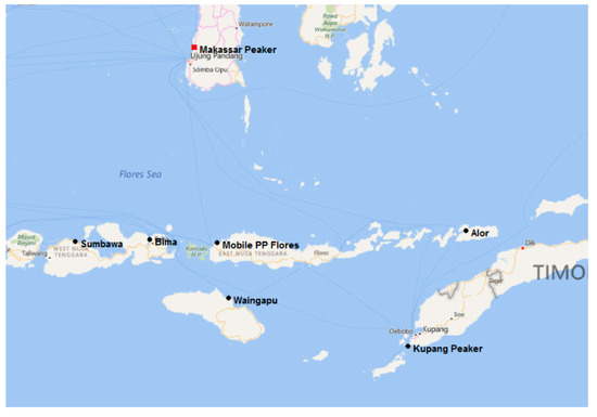
Figure 1.
Location of the supply port (Makassar Peaker) and the six receiving terminals in the Indonesian case study.

Table 1.
Ship-related parameters for the Indonesia case: Propulsion cost (), rental cost (), capacity (), traveling speed (), loading/unloading rate (), and berthing time ().
4.1.1. No Investment Costs, Time Horizon 5 × 14 Days
A five-period () formulation of the problem was applied with in each period, minimizing the total cost of the total time of 70 days. The routes of the optimal solutions are presented in the subpanels of Figure 2. One ship of Type 1 is used, but with different routes for each period. Load-splitting is only used once, i.e., in the third period (Makassar Peaker → Kupang Peaker → Mobile P.P. Flores) depicted in Figure 2c. One period serves a single customer (Sumbawa, in Figure 2d), two periods have two routes and two periods have three different routes. It should be noted that some trips are done twice (Sumbawa in the first, Kupang Peaker in the second, Bima in the third and fifth periods). The total distance traveled is 18,808 km, i.e., 269 km/d. As for the time use, reported in the caption of Figure 2, the ship is seen to be in use 10–14 days, except for the third period that only requires about 3 days. In total, the ship is in use for only about 50 days, so there is plenty of time left (in addition to the 2% time margin applied) to cope with possible delays. The volumetric shipping cost of the supply chain, which is minimized in the lack of land transportation and investment costs, is 22.13 €/m3 (equivalent to 3.80 €/MWh). A break-down of the costs is provided in the first result column of Table 2, which also reports the costs in the commonly used unit $US/MMBTU (The numbers are based on the currency conversion 1.0 € = $US1.21), where MMBTU expresses million of BTU and corresponds to about 293 kWh or 1055 MJ. (The second result column of the table represents the optimal solution of the case studied in Section 4.1.2).
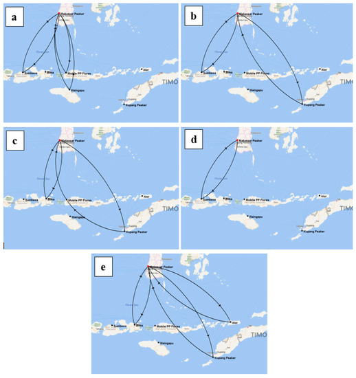
Figure 2.
Optimal routes for the multi-period problem in Indonesia with a time horizon of 5 × 14 days. The operation time of the ships are (a) 11.2 days, (b) 11.7 days, (c) 9.8 days, (d) 2.9 days, and (e) 13.7 days.
Table 2.
Shipping cost break-down for the multi-period Indonesia cases using time horizons of 5 × 14 days (left) and 5 × 10 days (right).
Other features of the solution are that two customers, the smallest ones (Alor and Waingapu), receive deliveries only once. The required tank sizes reported in the left column of Table 3 reveal the large requirement for sites that are supplied infrequently. Alor and Waingapu, which are supplied once, must (in addition to the heel) hold storages that last the whole 70-day period. A view of the levels in the tanks for the different periods is presented in Figure 3, which for the sake of clarity depicts the results for (=11) consecutive periods and has been split into two subpanels to make it easier to differentiate between the lines. The gradual decrease of the levels at Alor and Waingapu between the single charging points, as well as the more complex patterns shown by the levels in the tanks at Kupang P., Sumbawa, and in particular Mobile P.P. Flores are clearly seen. Even though the tank sizes of the other three sites are smaller than the total demand of the 70-day period, the tanks are still quite large as a consequence of disregarded investment costs.
Table 3.
Tank sizes for the multi-period Indonesia cases: 5 × 14 days without investment costs (left) and 5 × 10 days with investment costs (right).
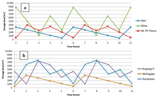
Figure 3.
Tank levels at (a) Alor, Bima and Mobile P.P. Flores and (b) Kupang Peaker, Waingapu and Sumbawa, at the beginning of the periods of the multi-period Indonesia case with a time horizon of . For clarity, consecutive periods are depicted.
4.1.2. Investment Costs, Time Horizon 5 × 10 Days
The poor time usage and the large tank sizes of the optimal solutions in Section 4.1.1 motivated a study where also the costs for the tanks were included in the objective function and the time-horizon was shortened to 5 × 10 days. The investment cost parameters and were used, applying a low-interest rate ( and a long project time ().
The optimal solution, presented in the subpanels of Figure 4, now shows much more complicated routes as the tank sizes affect the objective function. A majority of the routes apply load splitting, and the most complicated one even five times. The first and third periods (Figure 4a,c) apply identical routes, and one of their sub-routes (Makassar Peaker → Sumbawa → Bima) also appears in the fifth period (Figure 4e).
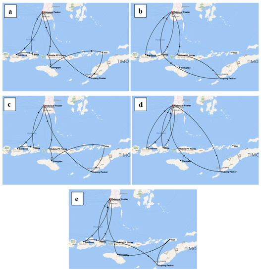
Figure 4.
Optimal routes for the multi-period problem in the case study of Indonesia, using a time horizon of 5 × 10 days. The operation time of the ships are (a) 9.4 days, (b) 8.6 days, (c) 9.4 days, (d) 9.8 days, and (e) 9.8 days.
The complex routes increase the daily distance traveled to 352 km/d (totaling 17,598 km on 50 days), but instead substantially decreases the required tank sizes. The rightmost column of Table 3 demonstrates that the tank sizes have been reduced to 1/4–1/3 of the sizes of the previous solution, i.e., much more than the shortened time horizon would imply. The shipping cost, in turn, increases (cf. rightmost columns of Table 2). The two subpanels of Figure 5 show much more uniform and lower LNG levels in the tanks. Two sites (Bima and Kupang Peaker) only have the required heel left after each period. This demonstrates how the added terms to the objective function have been effectively reduced by the optimization method. The routes are also seen to be well optimized with respect to time, reported in the caption of Figure 4.
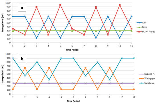
Figure 5.
Tank levels at (a) Alor, Bima and Mobile P.P. Flores and (b) Kupang Peaker, Waingapu and Sumbawa, at the beginning of the periods of the multi-period Indonesia case with a time horizon of . For clarity, consecutive periods are depicted.
4.2. Ship- and Truck-Based Supply Chain in a Coastal Region
The second example, where most of the features of the model are utilized, concerns a study of LNG delivery in the Gulf of Bothnia, i.e., the northern part of the Baltic Sea. The system studied was inspired by several LNG-related projects approved or under discussion in this region. A similar single-period LNG-supply chain optimization problem was presented in [7]. Two supply terminals (Tornio, Stockholm), one fixed satellite terminal (Pori, 30,000 m3), and three potential satellite terminals (Turku, Vaasa, Umeå) on the coasts of Finland and Sweden were preselected (Figure 6). In addition to these sites, 20 other demand clusters distributed in Finland and Sweden were identified as “inland” customers. The demands were assigned as gross estimates based on population, the extent of industrial activity, inspired by the analysis in earlier papers by the research group [7,20]. Five ship types, with capacities of 3000 m3, 5000 m3, 6500 m3, 7500 m3, and 10,000 m3 were considered, with parameters inspired by small-scale LNG carrier designs by Wärtsilä [21], as reported in Table 4. The sea and land distances are reported in Table A2 and Table A3 of the Appendix A. A maximum one-way traveling distance of was imposed for the port-customer road connections. The availability of vessels and trucks is a portion of the total time horizon, allowing for some extra time. Due to the shorter distances, a ship availability of 95% () was required, while the corresponding number for trucks was = 0.298; the latter factor also considers a rescaling of the total time to ten-hour working days in a five-day working week. The investment costs parameters of the (new) satellite terminals were set as in the Indonesian case. A port call fee of was imposed in the supply ports but no fee was used for the receiving ports. The supply ports were assumed to have an upper limit of LNG that they could provide daily, , but this was sufficient and was never approached for the cases studied. The LNG price at the two supply ports is identical, €/MWh, and the price of alternative fuel at the consumers is €/MWh. A berthing time of was applied in all ports, and the upper limit of truck visits per day at the terminals were for supply ports and for satellite ports. As for trucks, each has a capacity of 55 m3 (320.8 MWh), a purchase cost of , a traveling speed of and a cost of , and a filling/emptying time of The interest rate and project period were the same as in the Indonesian case. The problem results in 609 integers and 444 continuous variables and the solution time varied between some ten seconds to half an hour.
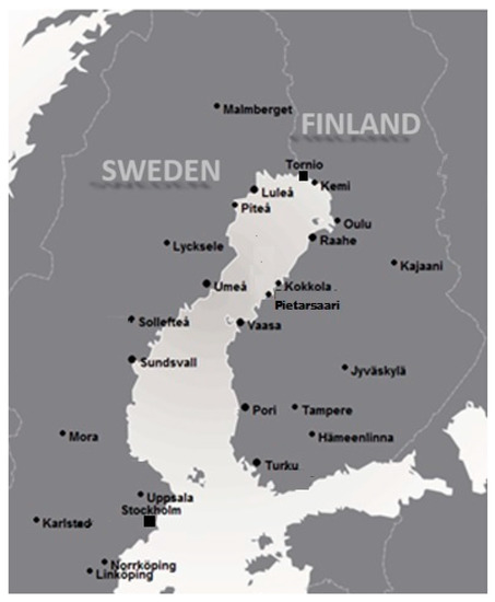
Figure 6.
Potential supply ports (solid squares), receiving terminals, and inland consumer clusters (solid circles) consider in the case study of the coastal region.
Table 4.
Ship-related parameters for the Gulf of Bothnia case: Propulsion cost, rental cost, capacity, traveling speed, loading/unloading rate, and the berthing time.
4.2.1. Single-Period Solution of the Gulf of Bothnia Case Study
The supply chain was first optimized for a single period of . Figure 7 illustrates the optimal maritime routing (curved arrowed arcs) and port-to-customer truck connections (straight arrowed lines). The energy demands are almost entirely satisfied by LNG: only two customers are partially supplied with alternative fuel (Sollefteå and Kokkola, both with 0.038 GWh). One ship of Type 3 (6500 m3) handles the LNG maritime distribution to the satellite terminals, which in addition to the one in Pori have been built in Umeå and Vaasa. The storage sizes of the latter ones are about 7500 m3 and 2500 m3, respectively. The maritime routing reported in Table 5 shows one split delivery between Umeå, Pori, and Vaasa. In total, 113.4 GWh of LNG is shipped to the satellite terminals; about one third from Stockholm and the rest from Tornio. LNG is transported by truck in 364 trips yielding a total energy supply of 113 GWh. Table 6 shows that the number of trucks per port ranges between 1 (Vaasa) and 17 (Tornio). The supply ports have the highest number as they serve a majority of the land customers they can reach. Quite expected, Pori shows the largest amount of trucked LNG among the satellite terminals and therefore also a high number of allocated trucks. The overall specific fuel cost for this solution is
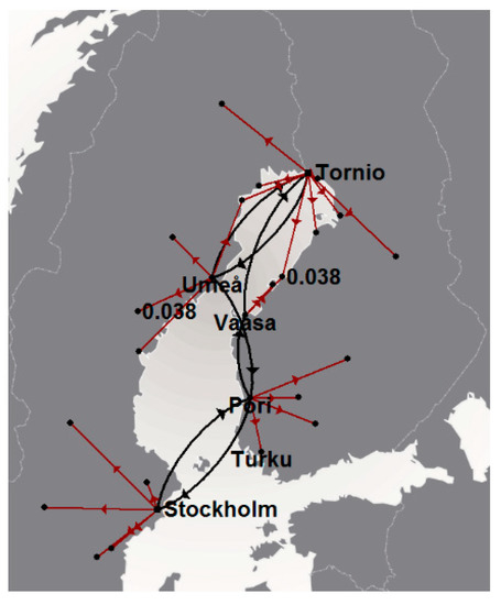
Figure 7.
Optimal satellite terminal locations and LNG distribution from supply to satellite ports and onward by land transportation for the single-period Gulf of Bothnia case. Straight arrows indicate land transport by truck and arrowed arcs maritime routing. The numbers in the figure denote alternative fuel used in GWh.
Table 5.
The optimal solution of the maritime routing for the single-period Gulf of Bothnia case, where denotes the number of trips and the shiploads.
Table 6.
Number of trucks per port and amount of liquefied natural gas (LNG) delivered to customers by truck in the single-period Gulf of Bothnia case.
As the LNG price at the supply ports is 30 €/MWh, the transportation and storage cost corresponds to 2.41 €/MWh ($US0.85/MMBTU).
4.2.2. Multi-Period Solution of the Gulf of Bothnia Case Study
The multi-period case considers three identical periods () with , i.e., a total time of 30 days. The land-based transport solution was taken to be identical for the time periods, so the amount of LNG delivered by truck, the number of trucks, and the related port-customers connections are the same in the three periods. However, they may differ from the solution of the single-period case, as the land-based transport was optimized together with the time-period-dependent maritime routing and storage.
Results of the optimization of the supply chain are presented in Figure 8 and Table 7 and Table 8. The same satellite terminals as in the single-period are built. However, the storage tanks are about 4000 m3 larger: 11,500 m3 in Umeå and 6500 m3 in Vaasa. The higher investment cost is compensated for by a shift to a smaller ship of Type 2, which is sufficient for the maritime LNG deliveries. Figure 8 and Table 7 present the routing, which is seen to differ between the periods. The total amount of LNG transported by ship is 341.8 GWh, supplied roughly equally from Stockholm and Tornio. The amount of LNG transported by trucks is 337.5 GWh. Compared to the results for the single-period problem, LNG deliveries by sea have increased by 0.5 GWh while deliveries by road have decreased by 0.5 GWh on average per period. LNG transported by truck from Tornio and Pori has decreased by 1.0 GWh and 3.2 GWh, respectively, while truck transport from Vaasa has increased by 3.7 GWh. This explains how the increase in maritime delivery has been used to partially outweigh the decrease in Tornio by redistributing the land-based deliveries between Pori and Vaasa (see Table 8). The remaining reduction in LNG use has been satisfied by larger quantities of alternative fuel (see numbers in Figure 8).
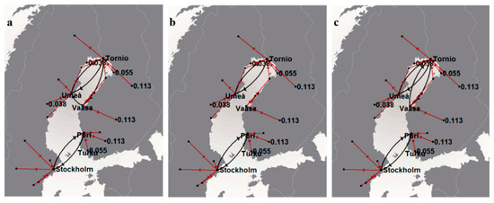
Figure 8.
Optimal satellite terminal locations and LNG distribution from supply to satellite ports and onward by land transportation for the multi-period Gulf of Bothnia case. (a) Period 1, (b) Period 2, and (c) Period 3. The numbers in the figure denote alternative fuel used in GWh.
Table 7.
Maritime routing in the optimal multi-period supply chain for the Gulf of Bothnia case.
Table 8.
Number of trucks per port and the amount of LNG delivered to customers by truck.
Figure 9 and Figure 10 illustrate how the storage tanks at the satellite terminals are used by depicting the volumes of LNG stored at the beginning of and the unloaded LNG volume during the time periods: a bigger inventory is used for periods when the unloaded LNG is insufficient to cover the demand. This is particularly the case for Vaasa, which has no ship visit during period 2 and instead uses the storage to satisfy the local demand and the demands of its associated inland customers (cf. Figure 8b). The specific cost for the multi-period solution is , which is almost 8 cents/MWh lower than the costs of the single-period solution, implying a saving of about 0.5 M€/a.
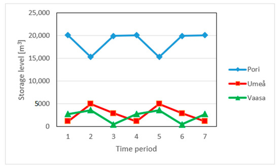
Figure 9.
The volume of LNG stored at the satellite terminals at the beginning of every time period of the multi-period Gulf of Bothnia case. For clarity, consecutive periods are depicted.
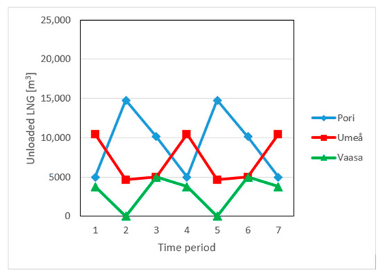
Figure 10.
Volume of LNG unloaded at the satellite terminals per time period of the multi-period Gulf of Bothnia case. For clarity, consecutive periods are depicted.
5. Conclusions
A model for designing optimal small-scale LNG supply chains has been presented. The model addresses both strategic and tactical aspects, which are often treated separately in the literature, by optimizing the delivery routes, quantities of LNG supplied, and the location and size of intermediate storage by simultaneous minimization of investment and operation costs. A multi-period formulation makes it possible to optimize the storage tank and inventory in the different time periods. The solution also gives the number and type of ships for the maritime supply and the number of tank trucks per port for the land-based deliveries. The ability of the model to tackle complex supply-chain design problems has been illustrated by two case studies. The advantage offered by a multi-period solution over a single-period solution in some cases was also demonstrated. The model can be used for initial planning and design of LNG supply chains, and the simplicity and flexibility of the model formulation also make it a versatile tool for sensitivity analysis or for analyzing “retrofit cases”, e.g., to evaluate potential upgrading of existing supply chains. In small-scale supply chains, where the demands are relatively small and the distances short, it is not clear at the outset whether, in terms of costs, operations should drive investment decisions or vice versa. Such questions can be clarified by using the model.
As an alternative to the present approach, a stochastic model could be developed to consider parameter variation and different scenarios to find robust solutions, i.e., insensitive to parametric changes to consider uncertainly in the design of the supply chain [22]. The ability of alternative solution strategies, e.g., evolutionary algorithms, will also be explored. Even though such methods are known to be inferior in terms of convergence (rate) they may constitute the only feasible alternative if the system tackled is of large complexity and size.
Author Contributions
Funding acquisition, H.S.; methodology, A.B.; supervision, H.S.; writing—original draft, A.B.; writing—review and editing, A.B. and H.S. All authors have read and agreed to the published version of the manuscript.
Funding
This work was partly carried out in the Efficient Energy Use (EFEU) research program coordinated by CLIC Innovation Ltd. with funding from the Finnish Funding Agency for Technology and Innovation (former Tekes, present Business Finland) and participating companies. The APC was funded by Åbo Akademi University.
Conflicts of Interest
The authors declare no conflict of interest.
Nomenclature
| Sets | Ship availability, | ||
| Inland customers | Overall specific fuel cost, €/MWh | ||
| Satellite terminals | Port call fee, € | ||
| Ship types | Price of alt. fuel, €/MWh | ||
| Customers | Price of LNG in supply port, €/MWh | ||
| Ports | Truck fuel consumption, €/km | ||
| Supply ports | Total costs, € | ||
| Time periods | Ship propulsion cost, €/km | ||
| Ship renting cost, €/d | |||
| Indices | Maritime distance between and , km | ||
| Inland customers, | Road distance between and , km | ||
| Satellite terminals, | Energy demand, MWh/d | ||
| Ship types, | Interest rate, | ||
| Customers, | Fraction of LNG storage capacity as heel, | ||
| Ports, | Time horizon, d | ||
| Supply ports, | Truck investment cost, € | ||
| Truck capacity investment cost, €/MWh | |||
| Variables * | Fixed satellite terminal investment cost, € | ||
| C, energy from alt. fuel, MWh | Big M parameter, | ||
| C, initial LNG inventory, MWh | Life length of investment, a | ||
| C, energy by trucked LNG, MWh | Number of time periods, | ||
| C, size of tank storage, MWh | Truck capacity, MWh | ||
| B, activation of the satellite terminal, | Ship capacity, MWh | ||
| C, ship loads transported, | Max. LNG available at supply port, MWh/d | ||
| I, number of routes , | Loading/unloading rate, MW | ||
| B, ship type, | Time of loading truck, h | ||
| I, number of truck per port, | Ship berthing time, h | ||
| I, number of truck trips , | Average travel speed of truck, km/h | ||
| Average cruising speed of ship, km/h | |||
| Parameters | Max. truck loads per day in port , 1/d | ||
| Truck availability, | Investment installment factor, 1/d | ||
| * B, I, and C denote binary, integer, and continuous variables, respectively. | |||
Appendix A
This Appendix reports the sea and land distances for the illustration cases of the paper. The marine distances in the Indonesian case (Table A1), studied in Section 4.1, were obtained by Wärtsilä. For the Gulf of Bothnia case, studied in Section 4.2, an online tool for calculation of distances between seaports [23] was applied to get the maritime distances (Table A2), while road distances (Table A3) were taken from a Google Maps [24]. The demands of the sites are reported on the last row of Table A1 and in the last column of Table A3, expressed in m3/d of LNG and GWh/d, respectively. A conversion of 1 m3 = 5.83 MWh was used in the calculations.
Table A1.
Sea distances () in km for the Indonesia case study and daily demand of LNG in the receiving ports.
Table A1.
Sea distances () in km for the Indonesia case study and daily demand of LNG in the receiving ports.
| Makassar | Alor | Bima | Kupang P | M. PP Flores | Sumbawa | Waingapu | |
|---|---|---|---|---|---|---|---|
| Makassar | 0 | 890 | 425 | 930 | 414 | 519 | 565 |
| Alor | 890 | 0 | 673 | 272 | 532 | 841 | 512 |
| Bima | 425 | 673 | 0 | 603 | 150 | 203 | 238 |
| Kupang P. | 930 | 272 | 603 | 0 | 594 | 780 | 383 |
| M. PP Flores | 414 | 532 | 150 | 594 | 0 | 327 | 222 |
| Sumbawa | 519 | 841 | 203 | 780 | 327 | 0 | 400 |
| Waingapu | 565 | 512 | 238 | 383 | 222 | 400 | 0 |
| (m3/d) | 54 | 272 | 244 | 109 | 272 | 54 |
Table A2.
Sea distances () in km [23] between ports in The Gulf of Bothnia case study.
Table A2.
Sea distances () in km [23] between ports in The Gulf of Bothnia case study.
| Tornio | Stockholm | Turku | Pori | Vaasa | Umeå | |
|---|---|---|---|---|---|---|
| Tornio | 0 | 809 | 885 | 559 | 373 | 338 |
| Stockholm | 809 | 0 | 324 | 422 | 580 | 632 |
| Turku | 885 | 324 | 0 | 315 | 485 | 452 |
| Pori | 559 | 422 | 315 | 0 | 253 | 288 |
| Vaasa | 373 | 580 | 485 | 253 | 0 | 115 |
| Umeå | 338 | 632 | 452 | 288 | 115 | 0 |
Table A3.
Road distances () in km between ports and customers (Google Maps) and customer daily demands of the Gulf of Bothnia case study.
Table A3.
Road distances () in km between ports and customers (Google Maps) and customer daily demands of the Gulf of Bothnia case study.
| Tornio | Stockholm | Turku | Pori | Vaasa | Umeå | GWh/d | |
|---|---|---|---|---|---|---|---|
| Turku | 778 | 1000 | 0 | 142 | 334 | 1163 | 1.0 |
| Pori | 639 | 455 | 142 | 0 | 191 | 1024 | 4.0 |
| Vaasa | 450 | 747 | 334 | 191 | 0 | 835 | 1.0 |
| Umeå | 386 | 638 | 1163 | 1024 | 835 | 0 | 3.0 |
| Kemi | 28 | 1050 | 752 | 612 | 424 | 413 | 0.7 |
| Kokkola | 330 | 868 | 436 | 309 | 121 | 1000 | 0.1 |
| Malmberget | 260 | 1138 | 1036 | 897 | 709 | 501 | 0.6 |
| Oulu | 131 | 1153 | 647 | 508 | 320 | 516 | 1.0 |
| Pietarsaari | 368 | 845 | 413 | 286 | 98 | 752 | 0.3 |
| Piteå | 175 | 850 | 951 | 813 | 624 | 213 | 0.3 |
| Jyväskylä | 470 | 622 | 308 | 263 | 267 | 1000 | 0.3 |
| Hämeenlinna | 658 | 456 | 143 | 186 | 321 | 441 | 0.3 |
| Kajaani | 313 | 1335 | 622 | 577 | 367 | 698 | 0.3 |
| Tampere | 618 | 476 | 162 | 111 | 240 | 360 | 0.5 |
| Uppsala | 957 | 70 | 1000 | 459 | 686 | 572 | 1.0 |
| Linköping | 1219 | 197 | 511 | 654 | 948 | 833 | 1.0 |
| Norrköping | 1182 | 160 | 474 | 617 | 911 | 797 | 1.0 |
| Karlstad | 1198 | 305 | 599 | 742 | 927 | 812 | 0.5 |
| Mora | 945 | 307 | 590 | 864 | 674 | 560 | 0.2 |
| Lycksele | 388 | 717 | 581 | 438 | 1000 | 128 | 0.5 |
| Sollefteå | 589 | 493 | 647 | 508 | 1000 | 203 | 0.1 |
| Raahe | 206 | 1228 | 563 | 434 | 246 | 591 | 1.2 |
| Luleå | 130 | 906 | 907 | 767 | 579 | 265 | 0.1 |
| Sundsvall | 649 | 375 | 1425 | 1285 | 1097 | 264 | 0.3 |
References
- Wood, D.A. A review and outlook for the global LNG trade. J. Nat. Gas Sci. Eng. 2012, 9, 16–27. [Google Scholar] [CrossRef]
- Becerra-Fernandez, M.; Cosenz, F.; Dyner, I. Modeling the natural gas supply chain for sustainable growth policy. Energy 2020, 205, 118018. [Google Scholar] [CrossRef]
- BP Energy Outlook. 2019. Available online: www.bp.com/content/dam/bp/business-sites/en/global/corporate/pdfs/energy-economics/energy-outlook/bp-energy-outlook-2019.pdf (accessed on 24 July 2020).
- Katebah, M.A.; Hussein, M.M.; Shazed, A.; Zineb, B.; Al-musleh, E.I. Rigorous simulation, energy and environmental analysis of an actual baseload LNG supply chain. Comput. Chem. Eng. 2020, 141, 106993. [Google Scholar] [CrossRef]
- Peng, P.; Lu, F.; Cheng, S.; Yang, Y. Mapping the global liquefied natural gas trade network: A perspective of maritime transportation. J. Clean. Prod. 2020, 124640. [Google Scholar] [CrossRef]
- Seithe, G.J.; Bonou, A.; Giannopoulos, D.; Georgopoulou, C.A.; Founti, M. Maritime transport in a life cycle perspective: How fuels, vessel types, and operational profiles influence energy demand and greenhouse gas emissions. Energies 2020, 13, 2739. [Google Scholar] [CrossRef]
- Bittante, A.; Jokinen, R.; Krooks, J.; Pettersson, F.; Saxén, H. Optimal design of a small-scale LNG supply chain combining sea and land transports. Ind. Eng. Chem. Res. 2017, 56, 13434–13443. [Google Scholar] [CrossRef]
- Bittante, A.; Pettersson, F.; Saxén, H. Optimization of a small-scale LNG supply chain. Energy 2018, 148, 79–89. [Google Scholar] [CrossRef]
- Braekers, K.; Ramaekers, K.; van Nieuwenhuyse, I. The vehicle routing problem: State of the art classification and review. Comput. Ind. Eng. 2016, 99, 300–313. [Google Scholar] [CrossRef]
- Hoff, A.; Andersson, H.; Christiansen, M.; Hasle, G.; Løkketangen, A. Industrial aspects and literature survey: Fleet composition and routing. Comput. Oper. Res. 2010, 37, 2041–2061. [Google Scholar] [CrossRef]
- Drexl, M.; Schneider, M. A survey of variants and extensions of the location-routing problem. Eur. J. Oper. Res. 2015, 283–308. [Google Scholar] [CrossRef]
- Andersson, H.; Hoff, A.; Christiansen, M.; Hasle, G.; Løkketangen, A. Industrial aspects and literature survey: Combined inventory management and routing. Comput. Oper. Res. 2010, 37, 1515–1536. [Google Scholar] [CrossRef]
- Li, M.; Schütz, P. Planning annual LNG deliveries with transshipment. Energies 2020, 13, 1490. [Google Scholar] [CrossRef]
- Baldacci, R.; Battarra, M.; Vigo, D. Valid inequalities for the fleet size and mix vehicle routing problem with fixed costs. Networks 2009, 54, 178–189. [Google Scholar] [CrossRef]
- Gonzalez-Feliu, J. The N-echelon Location Routing Problem: Concepts and Methods for Tactical and Operational Planning. 2009. Available online: https://halshs.archives-ouvertes.fr/halshs-00422492/file/Multi-echelon_LRP.pdf (accessed on 22 May 2020).
- Al-Khayyal, F.; Hwang, S.-J. Inventory constrained maritime routing and scheduling for multi-commodity liquid bulk, Part I: Applications and model. Eur. J. Oper. Res. 2007, 176, 106–130. [Google Scholar] [CrossRef]
- Koza, D.F.; Ropke, S.; Molas, A.B. The liquefied natural gas infrastructure and tanker fleet sizing problem. Transp. Res. E 2017, 99, 96–114. [Google Scholar] [CrossRef]
- Budiyanto, M.A.; Riadi, A.; Sumanta Buana, I.G.N.; Kurnia, G. Study on the LNG distribution to mobile power plants utilizing small-scale LNG carriers. Heliyon 2020, 6, e04538. [Google Scholar] [CrossRef] [PubMed]
- AIMMS-CPLEX. AIMMS-CPLEX. Available online: aimms.com/english/developers/resources/solvers/cplex (accessed on 12 June 2020).
- Jokinen, R.; Pettersson, F.; Saxén, H. An MILP Model for Optimization of a Small-scale LNG Supply Chain along a Coastline. Appl. Energy 2015, 138, 423–431. [Google Scholar] [CrossRef]
- Wärtsilä. Gas Carriers. 2015. Available online: www.wartsila.com/products/marine-oil-gas/ship-design/merchant/gas-carriers (accessed on 23 July 2020).
- Sangaiah, A.; Tirkolaee, E.B.; Goli, A.; Dehnavi-Arani, S. Robust optimization and mixed-integer linear programming model for LNG supply chain planning problem. Soft Comput. 2020, 24, 7885–7905. [Google Scholar] [CrossRef]
- Sea-Distances.org. SEA-DISTANCES.ORG—Distances. 2015. Available online: http://www.sea-distances.org/ (accessed on 12 May 2020).
- Google Maps. Google Maps. Available online: https://www.google.fi/maps?source=tldsi&hl=en (accessed on 2 April 2020).


Publisher’s Note: MDPI stays neutral with regard to jurisdictional claims in published maps and institutional affiliations. |
© 2020 by the authors. Licensee MDPI, Basel, Switzerland. This article is an open access article distributed under the terms and conditions of the Creative Commons Attribution (CC BY) license (http://creativecommons.org/licenses/by/4.0/).