Abstract
Gas hydrate saturation is an important index for evaluating gas hydrate reservoirs, and well logs are an effective method for estimating gas hydrate saturation. To use well logs better to estimate gas hydrate saturation, and to establish the deep internal connections and laws of the data, we propose a method of using deep learning technology to estimate gas hydrate saturation from well logs. Considering that well logs have sequential characteristics, we used the long short-term memory (LSTM) recurrent neural network to predict the gas hydrate saturation from the well logs of two sites in the Shenhu area, South China Sea. By constructing an LSTM recurrent layer and two fully connected layers at one site, we used resistivity and acoustic velocity logs that were sensitive to gas hydrate as input. We used the gas hydrate saturation calculated by the chloride concentration of the pore water as output to train the LSTM network. We achieved a good training result. Applying the trained LSTM recurrent neural network to another site in the same area achieved good prediction of gas hydrate saturation, showing the unique advantages of deep learning technology in gas hydrate saturation estimation.
1. Introduction
Gas hydrate is an ice-like crystalline solid, formed by water molecules and methane molecules under low temperature and high pressure. It is mainly distributed in seabed sediments on continental margins and permafrost regions. Gas hydrate can cause seabed geo-hazards and atmospheric environmental problems [1], but is also a clean energy with huge reserves [2]. Gas hydrate saturation is an important index for evaluating gas hydrate reservoirs. Well logs are widely used to estimate gas hydrate saturation due to their fast speed and low cost. The common methods for estimating the saturation of gas hydrate by using well logs mainly include resistivity methods and velocity methods [3]. Resistivity-based methods use resistivity logs to estimate gas hydrate saturation according to Archie’s law [4,5], while velocity-based methods use the theoretical or empirical relationship between gas hydrate saturation and velocity to estimate gas hydrate saturation by using velocity logs. The frequently used relationships between gas hydrate saturation and velocity include time-average equations [6], the effective medium theory [7,8], and three-phase Biot-type equations [9,10].
The close relationship between gas hydrate saturation and well log machine learning technology provides a new idea for using well logs to estimate gas hydrate saturation. Singh et al. [11,12] used different combinations of well logs to predict gas hydrate saturation through unsupervised and supervised machine learning algorithms. They obtained a higher accuracy of gas hydrate saturation than in classic resistivity and velocity methods, showing the advantages of machine learning technology in gas hydrate saturation predictions. As the most vigorous branch of machine learning, deep learning technology can achieve more accurate prediction and classification than traditional technology. This is because it builds a deep neural network model with multiple hidden layers and uses a lot of data to train the model to learn complex and effective information. Therefore, to use well logs better to estimate gas hydrate saturation and to establish the deep internal connections and laws of the data, we propose a method of estimating gas hydrate saturation from well logs by using deep learning technology.
The concept of deep learning first proposed by Hilton et al. [13] has been successfully applied in image, audio, and natural language processing, and its unique advantages have attracted increasing attention from geoscientists. Deep learning technology is being gradually applied to well log interpretation and reservoir prediction, such as in rock facies classification [14,15,16,17,18,19] and the prediction of shale content [20] and porosity [21]. Well logs are sequence samples, so to estimate the gas hydrate saturation, we adopted the long short-term memory (LSTM) recurrent neural network, which is suitable for processing sequential data to apply to the well logs that are sensitive to gas hydrate. This method brought good application results in the Shenhu area, South China Sea. It demonstrated the unique advantages of deep learning technology in gas hydrate saturation estimates, and laid the foundation for its further application in gas hydrate research.
2. Long Short-Term Memory (LSTM) Recurrent Neural Network
2.1. Recurrent Neural Network (RNN)
A recurrent neural network (RNN) is a neural network model with memory function that can discover the interrelationships between samples. It is especially used to process data with sequential characteristics. Unlike other network structures, an RNN introduces the idea of self-loop, which can input the output of the previous and next samples into the model for operation (Figure 1). The feature information processed by the model contains not only the information of the sequence data before the current sample, but also the information of the current sample itself. However, an RNN cannot effectively deal with long-term dependency problems (neurons that are far away in the hidden layer) because in the process of using the stochastic gradient descent method to train the RNN, the partial derivative of the loss function to the weight matrix will tend toward zero or infinity as the number of input sequence samples increases. This will bring problems of gradient vanishing or gradient exploding, limiting its wide application.
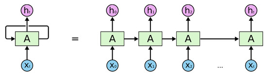
Figure 1.
Unfolded form of recurrent neural network [22].
2.2. LSTM Recurrent Neural Network
The LSTM network is a special recurrent neural network proposed by Hochreiter and Schmidhuber in 1997 [23]. It improves and perfects the loop body repeated in a chain in the conventional RNN. By adding a forget gate layer, an input gate layer, and an output gate layer in the network cell, continuous write, read, and reset operations on memory cells can be performed [24]. This enables LSTM to have long-term learning capabilities, and effectively solves the problems of gradient vanishing and gradient exploding, making it one of the most successful RNN networks. Figure 2 shows the basic network structure of LSTM, while Figure 3 shows the structure of an LSTM neuron.
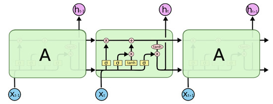
Figure 2.
The basic network structure of the long short-term memory (LSTM) network [22].
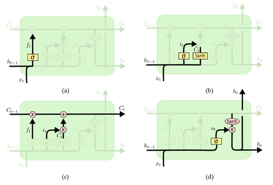
Figure 3.
The structure of an LSTM neuron [22]: (a) the forget gate layer, (b) the input gate layer, (c) the cell status, and (d) the output gate layer.
The forget gate layer of the LSTM network determines which information needs to be discarded (Figure 3). The expression is:
The input gate layer determines which new information is stored in the cell state (Figure 3b). The expression is:
Then, the current cell status (Figure 3c) is updated to:
The cell state of LSTM runs through the whole process, so that information is transmitted in a fixed and unchanging way. The output gate layer determines the information that needs to be output at that moment (Figure 3d). The expression is:
where is the input vector of the LSTM neuron; is the activation vector of the forget gate layer; is the activation vector of the input gate layer; is the output vector of the LSTM neuron; is the neuron cell state vector; is weight matrix; is the bias term; is the sigmoid function; (tanh) is the hyperbolic tangent function; the subscript indicates different moments.
3. Gas Hydrate Saturation Estimate
3.1. Geological Background
The Shenhu area is in the Pearl River Mouth Basin, in the middle of the northern slope of the South China Sea (Figure 4), and it is a key area for gas hydrate exploration. The water depth is 500–1500 m, the seabed topography is complicated, and the topographic slope varies greatly [25]. Since the late Miocene, with its gravity flow having developed and its high deposition rate, several kilometers of Mesozoic and Cenozoic sediments have accumulated to form enough organic matter to provide a source for gas hydrates [26]. In previous geological surveys of the area, many geophysical and geochemical markers indicating the existence of gas hydrates were discovered. In 2007, the Guangzhou Marine Geological Survey conducted the first gas hydrate drilling expedition in this area, and successfully drilled gas hydrate samples.
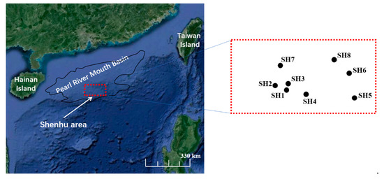
Figure 4.
The Pearl River Mouth Basin in the northern slope of the South China Sea; the Shenhu area is shown by the red rectangle.
3.2. Well Logs
Eight sites were drilled in the expedition area in 2007 (Figure 4). Gas hydrates were found in the cores of sites SH2, SH3, and SH7, but no hydrates were found at sites SH1 and SH5. The other three sites, namely, SH4, SH6, and SH9, were drilled for logging without cores.
Figure 5 shows the well logs of site SH2. The cores at this site confirmed that the gas hydrate-bearing sediments were in the range of 190–220 m, and the hydrate saturation could reach 47.3% [27].
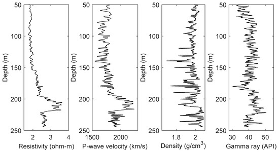
Figure 5.
Well logs at site SH2.
In the well logs of site SH2, the resistivity and acoustic velocity in the gas hydrate-bearing formations showed apparent high value anomalies, while the density and gamma showed no obvious changes. The well logs of site SH7 (Figure 6) showed that the depth of the gas hydrate-bearing formation was approximately 152–177 m, and the hydrate saturation could reach 43% [27]. The well log characteristics of the gas hydrate-bearing formation at site SH7 were completely consistent with those at site SH2.
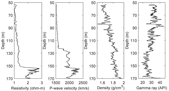
Figure 6.
Well logs at site SH7.
Gas hydrate causes the chloride concentration of the formation pore water to decrease, so the saturation of gas hydrate can be calculated by measuring the chloride concentration of pore water from cores [28] using:
where is the value of the density of pure gas hydrate in g/cm3. Here, is the in situ baseline pore water chloride concentration and is the measured chloride concentration in core water after gas hydrate dissociation. The baseline chloride concentration can be determined by smoothly fitting the chloride data above and below the gas hydrate zone [3].
Because the chloride concentration of the formation pore water was relatively less disturbed, and the chloride concentration measured by the cores was more accurate, the gas hydrate saturation calculated by the pore water chloride concentration had a higher accuracy [28]. Figure 7 shows the gas hydrate saturations calculated by using the chloride concentration measured by cores in the gas hydrate-bearing formation at sites SH2 and SH7. There were 41 gas hydrate-bearing cores at site SH2, and 21 cores containing gas hydrate at site SH7 [3,29].
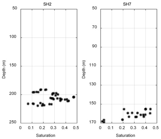
Figure 7.
Gas hydrate saturations calculated by the chloride concentration of the pore water from the cores at sites SH2 and SH7.
3.3. Data Preparation
To use the LSTM recurrent neural network to estimate the gas hydrate saturation, site SH2 was used as a training well to train the LSTM recurrent neural network, while site SH7 was used as a verification well to verify the accuracy of the network model. In site SH2, the resistivity and acoustic velocity, which are more sensitive to gas hydrate, were used as the input of the network model. The gas hydrate saturations calculated by the chloride concentration of the pore water in the cores were used as the output to train the LSTM recurrent neural network.
Because there were only 41 gas hydrate saturation values calculated from the chloride concentration at site SH2, too little training data would seriously affect the training effect of the LSTM recurrent neural network model. Therefore, the interpolation of the gas hydrate saturation was performed at the sampling interval of the well logs to obtain 1400 sample datasets in the range of 191–219 m (Figure 8) where the resistivity and the acoustic velocity were the input of the network model, and the interpolated gas hydrate saturation were output. Before the dataset was input to the LSTM recurrent neural network for training, 1000 consecutive samples were selected as the training dataset, with the remaining samples used as the test dataset. To eliminate the dimensional influence between the parameters, and to ensure that each parameter was within a reasonable distribution range, data standardization processing was required. The expression is:
where refers to the log parameters after standardization, refers to the input log parameters, and are the mean and standard deviation of the parameters, respectively.
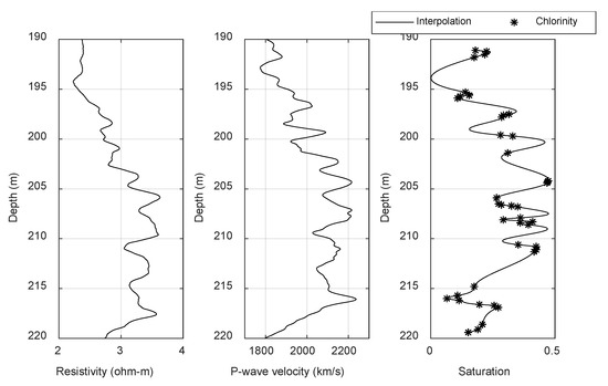
Figure 8.
Training dataset of the network model.
3.4. The Prediction Framework of the LSTM Recurrent Neural Network
We constructed an LSTM network prediction model that included an LSTM recurrent layer and two dense layers (Figure 9), where is the standardized input sequence sample of the resistivity and p-wave velocity; is the output saturation sample; LSTMi is the LSTM neuron that makes up the LSTM recurrent layer, which has the exact structure in Figure 3; is the output of the LSTM neuron; and have the same meanings as in Equations (1)–(5). Because the actual data were not particularly complicated, to improve the calculation efficiency, the number of nodes of the two fully connected layers was set to 20 and 10, respectively. The optimization algorithm adopted the Adam algorithm, and the dropout regularization method was used to prevent over-fitting.
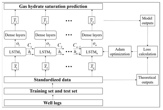
Figure 9.
The prediction framework of LSTM recurrent neural network.
The training process of the LSTM recurrent neural network was similar to that of a conventional fully connected neural network, namely: (1) Use feedforward propagation to input training data into the network, calculate the output of the LSTM unit, and then extract features through the two fully connected layers. This trains it layer by layer to the output layer to obtain the predicted estimate of this sample. (2) Back-calculate the error term of each neuron. The backward propagation of the error term of the LSTM recurrent neural network includes two directions: the first is the back propagation along time, that is, starting from the current time, calculating the error term at each time; the second is propagating the error term to the upper layer. (3) Use the Adam optimization algorithm based on gradient descent to adjust the model parameters by calculating the gradient of each weight according to the corresponding error item, so that the prediction is close to the optimization target. (4) Through the above iterations, train until it meets the required optimization target, then the LSTM recurrent neural network prediction model that meets the error requirements is established.
3.5. Results
Figure 10 shows the training results of the LSTM recurrent neural network using site SH2. The red dotted line shows the predicted saturation of the gas hydrate of the network model, and the blue curve shows the true value input into the model. The calculation shows that the correlation coefficient between the predicted value and the true value was 0.9605, and the root mean square error was 0.0208. The LSTM recurrent neural network achieved a good training effect, so it could be used for the prediction of gas hydrate saturation at site SH7.
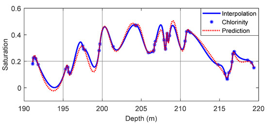
Figure 10.
Training results of the LSTM recurrent neural network at site SH2.
We selected the resistivity and acoustic velocity logs of 155–167 m at site SH7, standardized the data, and input the data into the previously trained LSTM recurrent neural network to obtain the prediction of the gas hydrate saturation (Figure 11). The black curve in Figure 11 shows the predicted value, and the black asterisks show the gas hydrate saturations calculated by the chloride concentration of the pore water at site SH7. The overall change trend of the predicted value of gas hydrate saturation obtained by the LSTM recurrent neural network was reasonable, and the prediction was basically consistent with the 21 measured values of site SH7. We picked out the corresponding 21 predicted values of gas hydrate saturation, and calculated the correlation coefficient and root mean square error between the predicted value and the true value. We obtained 0.7085 and 0.1208. We therefore achieved a relatively accurate prediction of gas hydrate saturation using the LSTM recurrent neural network.
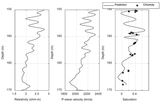
Figure 11.
Prediction of the gas hydrate saturation at site SH7.
4. Discussion
The design of the network structure is key to improving the accuracy of a network model. We used an LSTM network prediction model that included one LSTM recurrent layer and two fully connected layers. The number of nodes in the two fully connected layers was 20 and 10, respectively. We did this because the complexity of the actual data was relatively low and because we wanted to improve calculation efficiency. In addition to selecting parameters based on experience, the optimal network structure could also be selected by using the training dataset for repeated experiments. There are many ways to use dropout regularization in LSTM network training [30], either in the loop of LSTM or in the final fully connected layer. We chose to put dropout regularization in the fully connected layer.
The analysis of the cores in the Shenhu area showed that the gas hydrate-bearing sediments consisted of silt (70%), sand (<10%), and clays (15%–30%) [31]. Because the well logs of gas hydrate-bearing sediments were the comprehensive responses of lithology and gas hydrates, the log characteristics of gas hydrate-bearing sediments, with varying lithologies, were different. Therefore, the LSTM network trained by well logs is only suitable for gas hydrate saturation predictions of gas hydrate-bearing sediments with small lithological differences, such as adjacent sites in the same exploration area. For sites that are further apart, or located in other exploration areas, the predictions may have large errors.
5. Conclusions
Based on the successful application of machine learning technology in gas hydrate saturation using well logs, we proposed a method for estimating gas hydrate saturation from well logs using deep learning technology to establish the deep internal connections and laws of the data. Considering that well logs are sequence samples, this method designed the LSTM recurrent neural network to be suitable for processing sequential data, took the resistivity and acoustic velocity logs that are more sensitive to gas hydrates as input, took the gas hydrate saturation calculated by the chloride concentration as the output, and trained the LSTM recurrent neural network to accurately predict the saturation of gas hydrate. This method had higher accuracy prediction of gas hydrate saturation than traditional machine learning methods and achieved good application results in the two studied sites in the Shenhu area, South China Sea. It demonstrated the unique advantages of deep learning technology in gas hydrate saturation estimates, and laid the foundation for its further application in gas hydrate research.
Author Contributions
C.L. designed the experiments and wrote the paper; X.L. proposed the theory. All authors have read and agreed to the published version of the manuscript.
Funding
This research was funded by the National Natural Science Foundation of China (No. 41974153) and the Fundamental Research Funds for the Central Universities (No. 2652019038).
Acknowledgments
The design of this research was done by C.L. while he was a visiting scholar at the College of Earth, Ocean, and Atmospheric Sciences at Oregon State University. C.L. would like to thank Anne Tréhu for her providing the opportunity to work at Oregon State University.
Conflicts of Interest
The authors declare no conflict of interest.
References
- Ruppel, C.D. Tapping methane hydrates for unconventional natural gas. Elements 2007, 3, 193–199. [Google Scholar] [CrossRef]
- Archer, D. Methane hydrate stability and anthropogenic climate change. Biogeosci. Discuss. 2007, 4, 993–1057. [Google Scholar] [CrossRef]
- Wang, X.J.; Hutchinson, D.R.; Wu, S.G.; Yang, S.X.; Guo, Y.Q. Elevated gas hydrate saturation within silt and silty clay sediments in the Shenhu area, Souch China Sea. J. Geophys. Res. 2011, 116, B05102. [Google Scholar]
- Collett, T.S.; Ladd, J. Detection of gas hydrate with downhole logs and assessment of gas hydrate concentrations and gas volumes on the Blake Ridge with electrical resistivity log data. Proc. Ocean Drill. Program Sci. Results 2000, 164, 179–191. [Google Scholar]
- Lee, M.W.; Collett, T.S. Gas hydrate saturations estimated from fractured reservoir at Site NGHP-01-10, Krishna-Godavari Basin, India. J. Geophys. Res. 2009, 114, B07102. [Google Scholar] [CrossRef]
- Wood, W.T.; Stoffa, P.L.; Shipley, T.H. Quantitative detection of methane hydrate through high-resolution seismic velocity analysis. J. Geophys. Res. 1994, 99, 9681–9969. [Google Scholar] [CrossRef]
- Helgerud, M.B.; Dvorkin, J.; Nur, A.; Sakai, A.; Collett, T. Elastic-wave velocity in marine sediments with gas hydrates: Effective medium modeling. Geophys. Res. Lett. 1999, 26, 2021–2024. [Google Scholar] [CrossRef]
- Jakobsen, M.; Hudson, J.A.; Minshull, T.A.; Singh, S.C. Elastic properties of hydrate-bearing sediment using effective medium theory. J. Geophys. Res. 2000, 105, 561–577. [Google Scholar] [CrossRef]
- Carcione, J.M.; Gei, D. Gas-hydrate concentration estimated from P- and S-wave velocities at the Mallik 2L-38 research well, Mackenzie Delta, Canada. J. Appl. Geophys. 2004, 56, 73–78. [Google Scholar] [CrossRef]
- Carcione, J.M.; Tinivella, U. Bottom-simulating reflectors: Seismic velocities and AVO effects. Geophysics 2000, 65, 54–67. [Google Scholar] [CrossRef]
- Singh, H.; Seol, Y.; Myshakin, E.M. Prediction of gas hydrate saturation using machine learning and optimail set of well-logs. Comput. Geosci. 2020, 1–17. [Google Scholar] [CrossRef]
- Singh, H.; Seol, Y.; Myshakin, E.M. Automated Well-Log Processing and Lithology Classification by Identifying Optimal Features Through Unsupervised and Supervised Machine-Learning Algorithms. SPE J. 2020, 25. [Google Scholar] [CrossRef]
- Hinton, G.E.; Osindero, S.; The, Y.W. A fast learning algorithm for deep belief nets. Neural Comput. 2006, 18, 1527–1554. [Google Scholar] [CrossRef] [PubMed]
- Hall, B. Facies classification using machine learning. Lead. Edge 2016, 35, 906–909. [Google Scholar] [CrossRef]
- Bestagini, P.; Lipari, V.; Tubaro, S. A machine learning approach to facies classification using well logs. SEG Tech. Program Expand. Abstr. 2017, 2137–2142. [Google Scholar] [CrossRef]
- Zhang, L.; Zhan, C. Machine learning in rock facies classification—An application of XGBoost. Int. Geophys. Conf. Qingdao China. 2017, 1371–1374. [Google Scholar] [CrossRef]
- Hall, M.; Hall, B. Distribution collaborative prediction: Results of the machine learning contest. Leading Edge 2017, 36, 267–269. [Google Scholar] [CrossRef]
- Sidahmed, M.; Roy, A.; Sayed, A. Streamline rock facies classification with deep learning cognitive process. SPE Annu. Technical Conf. Exhib. 2017. [Google Scholar] [CrossRef]
- An, P.; Cao, D. Research and application of logging lithology identification based on deep learning. Prog. Geophys. 2018, 33, 1029–1034. (In Chinese) [Google Scholar]
- An, P.; Cao, D. Shale content prediction based on LSTM recurrent neural network. In Proceedings of the SEG 2018 Workshop: SEG Maximizing Asset Value Through Artificial Intelligence and Machine Learning, Beijing, China, 17–19 September 2018; pp. 49–52. [Google Scholar]
- An, P.; Cao, D.; Zhao, B.; Yang, X.; Zhang, M. Reservoir physical parameters prediction based on LSTM recurrent neural network. Prog. Geophys. 2019, 34, 1849–1858. (In Chinese) [Google Scholar]
- Sofiyanti, N.; Fitmawati, D.I.; Roza, A.A. Understand LSTM Networks. GITHUB Colah Blog 2015, 22, 137–141. [Google Scholar]
- Hochreiter, S.; Schmidhuber, J. Long short-term memory. Neural Comput. 1997, 9, 1735–1780. [Google Scholar] [CrossRef]
- Graves, A. Supervised Sequence Labelling with Recurrent Neural Networks; Springer: Berlin/Heidelberg, Germany, 2012. [Google Scholar]
- Briais, A.; Patriat, P.; Tapponnier, P. Updated interpretation of magnetic anomalies and seafloor spreading stages in the South China Sea: Implications for the tertiary tectonics of Southeast Asia. J. Geophys. Res. 1993, 98, 6299–6328. [Google Scholar] [CrossRef]
- Clift, P.; Lin, J.; Barckhausen, U. Evidence of low flexural rigidity and low viscosity lower continental crust during continental break-up in the South China Sea. Mar. Pet. Geol. 2002, 19, 951–970. [Google Scholar] [CrossRef]
- Wang, X.; Collett, T.S.; Lee, M.W.; Yang, S.; Guo, Y.; Wu, S. Geological controls on the occurrence of gas hydrate from core, downhole log, and seismic data in the Shenhu are, South China Sea. Mar. Geol. 2014, 357, 272–292. [Google Scholar] [CrossRef]
- Yuan, T.; Hyndman, R.D.; Spence, G.D.; Desmons, B. Seismic velocity increase and deep-sea gas hydrate concentration above a bottom-simulating reflector on the northern Cascadia continental slope. J. Geophys. Res. 1996, 101, 655–671. [Google Scholar] [CrossRef]
- Chen, Y.; Dunn, K.; Liu, X.; Du, M.; Lei, X. New method for estimating gas hydrate saturation in the Shenhu area. Geophysics 2014, 79, IM11–IM22. [Google Scholar] [CrossRef]
- Gal, Y.; Ghahramani, Z. A theoretically grounded application of dropout in recurrent neural networks. arXiv 2015, arXiv:1512.05287. [Google Scholar]
- Chen, F.; Zhou, Y.; Su, X.; Liu, G.; Lu, H.; Wang, J. Gas hydrate saturation and its relation with grain size of the hydrate-bearing sediments in the Shenhu Area of northern South China Sea. Mar. Geol. Quat. Geol. 2011, 31, 95–100. (In Chinese) [Google Scholar] [CrossRef]


Publisher’s Note: MDPI stays neutral with regard to jurisdictional claims in published maps and institutional affiliations. |
© 2020 by the authors. Licensee MDPI, Basel, Switzerland. This article is an open access article distributed under the terms and conditions of the Creative Commons Attribution (CC BY) license (http://creativecommons.org/licenses/by/4.0/).