Application of Equilibrium Optimizer Algorithm for Optimal Power Flow with High Penetration of Renewable Energy

Abstract

In recent decades, the energy market around the world has been reshaped to accommodate the high penetration of renewable energy resources. Although renewable energy sources have brought various benefits, including low operation cost of wind and solar PV power plants, and reducing the environmental risks associated with the conventional power resources, they have imposed a wide range of difficulties in power system planning and operation. Naturally, classical optimal power flow (OPF) is a nonlinear problem. Integrating renewable energy resources with conventional thermal power generators escalates the difficulty of the OPF problem due to the uncertain and intermittent nature of these resources. To address the complexity associated with the process of the integration of renewable energy resources into the classical electric power systems, two probability distribution functions (Weibull and lognormal) are used to forecast the voltaic power output of wind and solar photovoltaic, respectively. Optimal power flow, including renewable energy, is formulated as a single-objective and multi-objective problem in which many objective functions are considered, such as minimizing the fuel cost, emission, real power loss, and voltage deviation. Real power generation, bus voltage, load tap changers ratios, and shunt compensators values are optimized under various power systems’ constraints. This paper aims to solve the OPF problem and examines the effect of renewable energy resources on the above-mentioned objective functions. A combined model of wind integrated IEEE 30-bus system, solar PV integrated IEEE 30-bus system, and hybrid wind and solar PV integrated IEEE 30-bus system is performed using the equilibrium optimizer technique (EO) and other five heuristic search methods. A comparison of simulation and statistical results of EO with other optimization techniques showed that EO is more effective and superior and provides the lowest optimization value in term of electric power generation, real power loss, emission index and voltage deviation.

1. Introduction

1.1. Background

The urgent need for reducing the fuel cost of the conventional power generation units and minimizing the greenhouse gases emitted from the thermal power generators have led various electric power companies to go toward utilizing renewable energy resources. Furthermore, the advanced technologies of renewable energy resources have contributed significantly to them becoming the most inexpensive and environmentally friendly resources. Integrating wind and solar PV in proper locations and appropriate settings of the variables of the conventional power networks may have a significant impact on the performance of power system control and operation.

To make the modeling of wind and solar PV more accurate and realistic, the Weibull probability distribution function was used to forecast the wind speed [1,2], whereas lognormal probability distribution function was used to mimic the intermittent nature of solar irradiance in [3,4].

1.2. Literature Review

Numerous publications in the literature studied the optimal power flow (OPF) problem for systems consisting of conventional power generation and renewable energy power plants. Deterministic, stochastic or hybrid optimization methods are used extensively to address the issues associated with increased penetration of non-dispatchable renewable energy, advanced controls such as FACTS devices and deregulated electricity markets.

Various conventional optimization techniques are used to solve the OPF problem. For instance, continuous nonlinear programming (NLP) was proposed [5]. The main advantage of NLP is that it is easily applied for solving large-scale power systems but it does not consider all of the system components. An extended conic quadratic format [6] is presented to solve the economic dispatch and decrease real power loss. Besides, the predictor-corrector interior point algorithm (PCIP) is proposed to fit the OPF for solving nonlinear programming problems [7]. Quadratic programming (QP) is used to derive a loss formula based on the incremental power flow. QP’s main advantages are that it does not require the calculation of the gradient steps, it is more accurate than linear and non-linear programming, and QB is also applicable in ill-conditions problem [8]. Sequential quadratic programming (SQP) is used to address large scale OPF; it also depends on transforming the original problem to a sequence of a linearly constrained sub-problem by applying an augmented Lagrangian [9]. Mixed integer linear programming (MILP) are adapted to minimize transmission losses and reactive generator outputs. MILP can provide the most accurate way to represent power system with a discrete control parameter. However, the main drawback of MILP is the presence of a strong trade-off between the accuracy of the system and the tractability of the problem [10]. Although these methods have excellent convergence characteristics, they have various drawbacks, including failing to find the global solution because of non-convexity and facing difficulty while handling the problems with non-differentiable and discontinuous objective functions.

Recently, metaheuristic optimization algorithms have been gaining much attention due to flexibility, free of derivation, and local optima avoidance. Thus, single and multi-objective optimization methods overcome the shortcomings attributed to classical techniques. A gravitational search algorithm (GSA) to find the optimal solution for OPF and IEEE 30-bus and 57-bus systems are examined. One of the most significant merits of GSA is the gravitational constant which has the ability to adjust the accuracy of the search to speed up the solution process. Another advantage, GSA is a memory-less method but it can work effectively similarly to algorithms with memory [11]. The basic fuel cost, voltage profile, voltage stability, and non-smooth quadratic cost are minimized and optimized using a differential evolution algorithm (DE). This approach has various benefits, including simple encoding, integer discrete handling, fast convergence and optimal solution identification [12]. The black hole-based optimization method is used to address the OPF problem for IEEE 30-bus and Algerian 59-bus power systems; simplicity and the parameter-free aspect are the main two benefits of this method over well-known optimization techniques [13]. Constrained OPF problem for IEEE 30-bus, 57-bus, and 118-bus is optimized using a moth swarm algorithm [14]. A multi-objective OPF to minimize the generation cost and environmental pollution using a fuzzy membership function to choose a compromise solution from the Pareto optimal solutions is discussed [15]. The fuel cost, voltage deviation, and real power loss are minimized as a multi-objective OPF problem using a gravitational search algorithm [16]. A modified teaching learning-based optimization algorithm (MTLBO) added a self-adapting wavelet mutation strategy and a fuzzy clustering. MTLBO provides a self-adaptive wavelet to improve the search capability, diversity and convergence speed. Moreover, a fuzzy decision making method is applied to sort the solution according to their significance. Finally, a smart population selection is included to select the population of the next iterations of the algorithms [17]. A hybrid of fuzzy evolutionary and swarm optimization is proposed to minimize the cost of active power generation and real power losses [18].

A fuzzy-based modified bee colony (MABC) is presented to solve discrete OPF using multi-objective mixed integer nonlinear. Furthermore, it is proven that MABC is more effective in finding the global search exploration than original bee colony and it also does not degrade while solving the higher dimension power systems [19]. Emission, real power losses, and voltage deviation are all minimized as a multi-objective OPF using a multi-objective modified imperialist competitive algorithm. This new technique is strong, effective and fast in comparison with the original imperialist competitive algorithm [20]. The particle swarm optimization and the shuffled frog leaping algorithm are hybridized to solve OPF using the generator’s constraints, such as prohibited zones and valve point effect.This method can successfully increase the diversity of generating population by adding four dominant strategies to move each individual of the existing swarm [21]. A chaotic invasive weed optimization algorithm is proposed to solve the OPF problem with non-smooth and non-convex fuel cost curves. The difficulties that the original invasive weed optimization algorithm faces in order to reach a better optimal solution were addressed. Additionally, this method is more stable and suitable for non-linear OPF [22]. Brain storming optimization (BSO) and teaching-learning optimization(TLBO) are hybridized to minimize the fuel cost of thermal generation units; this method outperforms TLBO and BSO, owing to a self evolving principle which is applied to the control parameter and a higher memory capability during its intermediate stages [23]. A hybrid optimization algorithm is based on sequential quadratic programming (SQP) to generate an initial population. Then, a differential evolution(DE) took that population to find the optimal solution more effectively and it was used to minimize the fuel cost with valve point and the transmission line real losses, the unfavorable results of DE which include stagnation and premature convergence can be avoided through benefiting from the impressive role of SQP in relaxing the discrete variables of the system [24].

A growing and considerable effort have been made in recent years to solve and model the OPF problem, including renewable energy sources. The OPF problem with taking into account uncertainties in the wind, solar, and load forecast and optimized using a genetic algorithm and two-point estimate method is presented in [25]. A hybrid method called moth swarm algorithm and gravitational search algorithm is used to solve the problem of OPF, including wind power [26]. A modified two-point estimation method is used to solve probabilistic OPF incorporating wind and solar photovoltaic power [27]. Hybrid wind photovoltaic power systems are optimized using the unscented transformation method, which can carry out probabilistic OPF with high accuracy and less computational time [28]. The OPF, including wind, is optimized using a fuzzy-based particle swarm optimization. A fuzzy set modeled the forecast load demand and wind speed [29].

Besides, OPF incorporating wind power energy is optimized by a hybrid algorithm called a hybrid dragonfly with aging particle swarm optimization [30]. Adaptive differential evolution with proper constraint handling method is addressed OPF, including wind and solar. The forecast wind and solar photovoltaic are modeled using Weibull and lognormal probability distribution functions [4]. An optimal reactive power dispatch with solar photovoltaic power and its impact on minimizing real power losses is addressed using the Jaya algorithm to solve this issue [31]. A constrained multi-objective population external optimization method in [32] is presented to minimize the fuel cost and emission in the presence of renewable energy sources. A grey wolf optimization algorithm (GWO) in [33] was proposed to tune the parameters of a thyristor controlled series compensator and address OPF, including wind and solar power. A best guided artificial bee colony optimization in [1] was to find the optimal setting of conventional and renewable power generation.

1.3. Contribution and Paper Organization

In the present work, an equilibrium optimizer [34], which is a novel optimization method inspired by controlling the volume mass balance model for estimating both equilibrium and dynamic states, is used to prove its performance in solving the OPF problem. It is implemented on (i) IEEE 30-bus system, (ii) wind integrated IEEE 30-bus system, (iii) solar PV integrated IEEE 30-bus system, and (iv) hybrid wind and solar PV integrated IEEE 30-bus system. Real power loss minimizations, total cost minimization of generating units and emission index minimization are considered to be the objective functions of the OPF problem. Weibull and lognormal probability distribution functions are used to model the wind speed and solar irradiance to forecast the output power of wind and solar PV systems. Furthermore, aiming to fill the gap in the literature, this paper investigates the impact of the presence of only wind or only solar PV or both of them on enhancing the objective functions of the OPF problem. In addition, a comprehensive statistical analysis for the equilibrium optimizer technique (EO) and other optimization techniques are used.

The rest of this paper is organized as follows: the formulation of OPF problem is described in Section 2. Then, a mathematical model of wind and solar PV plants is introduced in Section 3. Section 4 presents the equilibrium optimizer technique (EO) and its implementation to solve the OPF problem. Section 5 presents the test systems and the input parameters of the test systems and the optimization methods. Simulation results are explained in Section 6. Finally, Section 7 draws the conclusion of this work.

2. Problem Formulation of OPF

2.1. General Structure of OPF

Generally, OPF aims to minimizes some objective functions. $f_o$ is the objective function to be minimized, and h and g are the equality and inequality constraints in the power system network; OPF can be expressed as [14,35]:

$$\begin{array}{ccc}\mathrm{M}\mathrm{i}\mathrm{n}\mathrm{i}\mathrm{m}\mathrm{i}\mathrm{z}\mathrm{e}\hfill & f_o(\mathit{x},\mathit{u})\hfill & \\ \mathrm{s}\mathrm{u}\mathrm{b}\mathrm{j}\mathrm{e}\mathrm{c}\mathrm{t} \mathrm{t}\mathrm{o}\hfill & g(\mathit{x},\mathit{u})\le 0\hfill & \\ \hfill & h(\mathit{x},\mathit{u})=0\hfill & \end{array}$$

(1)

x is a state vector of dependent variables including the real power of swing generator ($P_{G_1}$), ($V_{L_i}$) is the voltage magnitude of load buses, ($Q_{G_i}$) is the reactive power of generator at $i_{th}$ bus and ($S_{l_i}$) is the loading of the $i_{th}$ transmission line. x can be expressed as follows [14,35]:

$$x={[P_{G_1},V_{L_1},\dots ,V_{L_{npq}},Q_{G1},\dots ,Q_{G_{NG}},S_{l_1},\dots ,S_{l_{n_l}}]}^T$$

(2)

where $npq$ and $n_l$ are the number of PQ buses and transmission lines. $S_l$ and $n_l$ are the loading of transmission lines and the number of transmission lines, respectively.

u is a vector consisting of control variables, ($P_{G_i}$) is the real power of all generators excluding swing generator, ($V_{G_i}$) is the voltage magnitude of generators, ($TS$) is the branch transformer tap, and ($Q_C$) is the shunt capacitor. u can be expressed as follows [14,35]:

$$u={[P_{G_2},\dots ,P_{G_{NG}},V_{G_1},\dots ,V_{G_{NG}},Q_{C1},\dots ,Q_{C{N}_c},T{S}_1,\dots ,T{S}_{N_T}]}^T$$

(3)

where, $NG$, $N_c$ and $N_T$ are the number of generators, shunt VAR compensator and transformers, respectively.

2.2. Objective Functions of OPF

Here, the first four cases dealt with solving single objective OPF and the last one addressed the multi-objective OPF.

• Case 1: real power loss minimization
  Due to the presence of the inherent resistance for the transmission lines, the aim of this function is to minimize the active power losses and it is expressed as [14,35]:

  $$f_o(x,u)=P_{loss}=\sum _{q=1}^{nl}{G}_{q_{(ij)}}(V_i^2+V_j^2-2V_i{V}_{j}cos({\delta }_{ij}))$$

  (4)

  where $G_{q(ij)}$ is the conductance of $q_{th}$ transmission line, and $V_i$ and $V_j$ are the voltage magnitude of terminal buses of transmission line.
• Case 2: emission index minimization
  In the present case, the target is to reduce the harmful gases emission from the thermal generation units, and the coefficients of the gas emission of the thermal power generators are given in Table 1. Emission in tons per hour (t/h) can be described by [14,35]:

  $$f_o(x,u)=E=\sum _{i=1}^{NG}[({\alpha }_i+{\beta }_i{P}_{G_i}+{\gamma }_i{P}_{G_i}^2)\ast 0.01+{\omega }_{i}e{(}^{\mu i{P}_{G_i}})]$$

  (5)

  where $\alpha$, $\beta$, $\gamma$, $\omega$ and $\mu$ are the emission coefficients and G1, G2, G3, G4, G5, and G6 represent thermal power generators at buses 1, 2, 5, 8, 11, and 13, respectively, as given in Table 1.
  Table 1. Emission coefficients of thermal power generating units [14,35].

  Generator	Bus	$\mathit{\alpha }$	$\mathit{\beta }$	$\mathit{\gamma }$	$\mathit{\omega }$	$\mathit{\mu }$
  G1	1	4.091	−5.554	6.49	0.0002	2.857
  G2	2	2.543	−6.047	5.638	0.0005	3.333
  G3	5	4.258	−5.094	4.586	0.000001	8
  G4	8	5.326	−3.55	3.38	0.002	2
  G5	11	4.258	−5.094	4.586	0.000001	8
  G6	13	6.131	−5.555	5.151	0.00001	6.667

• Case 3: Basic fuel cost minimization
  The relationship between fuel cost ($\$/h$) and the power generated from the thermal generating units can be approximately given by the quadratic relationship and it is expressed as [14,35]:

  $$f_o(x,u)=FC=\sum _{i=1}^{NG}{a}_i+b_i{P}_{G_i}+c_i{P}_{G_i}^2$$

  (6)

  where $a_i$, $b_i$, $c_i$ are the cost coefficient of the thermal generators and these coefficients are provided in Table 2.
  Table 2. Cost coefficients of the thermal power generators [14,35].

  Generator	Bus	a	b	c
  G1	1	0	2	0.00375
  G2	2	0	1.75	0.0175
  G3	5	0	1	0.0625
  G4	8	0	3.25	0.00834
  G5	11	0	3	0.025
  G6	13	0	3	0.025

• Case 4: Voltage deviation minimization
  The voltage deviation index is the cumulative deviation of all load buses from nominal value of unity. It also plays a significant role in keeping the voltage quality and security of the electrical power network.This case is expressed as [14,35]:

  $$f_o(x,u)=VD=\left(\sum _{p=1}^{NL}|V_{L_p}-1|\right)$$

  (7)
• Case 5: Minimization of basic the fuel cost, emission index, voltage deviation and the real power losses.
  The aim of this case is to reduce quadratic fuel cost, active power transmission losses, environmental emission index and voltage deviation index simultaneously. It can be defined as follows [14,35]:

  $$f_o(x,u)=FC+{\lambda }_p\times P_{loss}+{\lambda }_{VD}\times VD+{\lambda }_E\times E$$

  (8)

  where ${\lambda }_p$, ${\lambda }_{VD}$ and ${\lambda }_E$ are weight factors and they are assumed to be 22, 21 and 19, respectively as in [14].

2.3. Constraints

The constraints of OPF are usually categorized into [14,35]:

• Equality constraints
  The equality constraints of OPF are usually represented by the load flow equations:

  $$P_{G_i}-P_{D_i}=V_i\sum _{k=1}^{N_B}{V}_k(G_{ik}cos{\theta }_{ik}+B_{ik}sin{\theta }_{ik})$$

  (9)

  $$Q_{G_i}-Q_{D_i}=V_i\sum _{k=1}^{N_B}{V}_k(G_{ik}sin{\theta }_{ik}-B_{ik}cos{\theta }_{ik})$$

  (10)

  where $P_{D_i}$, $Q_{D_i}$, $N_B$, and ${\theta }_{ik}$ are the active and reactive load demand, the number of buses and the angle difference between bus i and k, respectively. $G_{ik}$ and $B_{ik}$ are the transfer and susceptance conductance.
• Inequality constraints
  It can be defined by operating limits on the equipment of the power system, transmission loading and voltage of load buses.

  (a)

  Constraints of thermal and renewable energy generating units

  $$V_{G_{i,min}}\le V_{G_i}\le V_{G_{i,max}}i=1,\dots ,N$$

  (11)

  $$P_{G_{i,min}}\le P_{G_i}\le P_{G_{i,max}}i=1,\dots ,N$$

  (12)

  $$Q_{G_{i,min}}\le Q_{G_i}\le Q_{G_{i,max}}i=1,\dots ,N$$

  (13)

  (b)

  Constraints of the transformer tap setting

  $$T{S}_{k,min}\le T{S}_k\le T{S}_{k,max}k=1,\dots ,N_T$$

  (14)

  (c)

  constraints of the shunt compensator

  $$Q_{C,j,min}\le Q_C\le Q_{C,j,max}j=1,\dots ,N_C$$

  (15)

  (d)

  Constraints of the voltages at load buses

  $$V_{Lr,min}\le V_{Lr}\le V_{Lr,max}r=1,\dots ,N_L$$

  (16)

  (e)

  Constraints of the transmission line loading

  $$S_{lv}\le S_{lv,max}v=1,\dots ,n_l$$

  (17)

2.4. Constraint Handling

In order to decline the infeasible solutions of OPF and keep the dependent variables within the allowable ranges, a penalty function was modeled and added to the objective functions defined in Section 2.2 [14,35].

$$penalty=K_p{(P_{G1}-P_{G1}^{Lim})}^2+K_Q\sum _{i=1}^{NG}{(Q_{Gi}-Q_{Gi}^{Lim})}^2+K_V\sum _{i=1}^{NL}{(V_{Li}-V_{Li}^{Lim})}^2+K_S\sum _{i=1}^{nl}{(S_{li}-S_{Li}^{Lim})}^2$$

(18)

where $K_Q$, $K_p$, $K_V$ and $K_S$ are the values of penalty factors associated with generation reactive power, generation real power of the swing generator, load bus voltages and line flow of transmission lines. They are assumed to be 100, 100, 100, and 100,000, respectively [14,36], and $x^{Lim}$ is the value of the violated limit of dependent variables(x). It is equal to $x^{max}$ in case of $x>x^{max}$ or $x^{min}$ in case of $x<x^{min}$.

3. Mathematical Models of the Wind and Solar Power Generating Units

3.1. Wind Power Units

3.1.1. Uncertain and Power Model of Wind Turbines

The wind speed of the wind turbines follows the Weibull probability distribution function. The characteristic of the output power generated by the wind turbine is a random variable depending on wind speed. The Weibull probability distribution function with dimensionless shape factor (k) and scale factor (c) is used to model the wind speed $f_v(v)$. The wind speed ($f_v(v)$) can be expressed mathematically as [1,2,37,38]:

$$f_v(v)=\frac{k}{c}{\left(\frac{v}{c}\right)}^{k-1}\times e^{-{\left(\frac{v}{c}\right)}^k}$$

(19)

The electrical energy generated by a wind turbine is the result of converting the kinetic energy of wind. The actual output power of wind turbines $(P_w(v))$ can be presented as [1,2,37,38]:

$$P_w(v)=\left\{\begin{array}{cc}0\hfill & v<v_{in}andv>v_{out}\hfill \\ P_{wr}\left({\displaystyle \frac{v-v_{in}}{v_r-v_{in}}}\right)\hfill & v_{in}\le v\le v_r\hfill \\ P_{wr}\hfill & v_r<v\le v_{out}\hfill \end{array}\right.$$

(20)

where $(P_{wr})$, $(v_{in})$, $(v_{out})$ and $(v_r)$ are the rated power of the wind turbine, the cut-in wind speed of the wind turbine, the cut-out wind speed and the rated wind speed, respectively.

3.1.2. Calculation of Direct, Underestimation and Overestimation Cost of Wind Power

The direct cost of wind power plant can be defined as [4,39,40,41]:

$$C_{w,j}(P_{ws,j})=g_j{P}_{ws,j}$$

(21)

where $g_j$ is the direct cost coefficient of wind plant.

The cost function is overestimated because the actual generated power from the wind turbine is less than the estimated power by mathematical equations. The overestimation cost is used for reverse the requirements when the estimated output power of the wind turbine is more than actual output power. Reserve cost for the $j^{th}$ wind turbine can be defined as [4,39,40,41]:

$$\begin{array}{c}\hfill C_{Rw,j}(P_{ws,j}-P_{wav,j})=K_{Rw,j}(P_{ws,j}-P_{wav,j})\\ \hfill =K_{Rw,j}{\int }_0^{P_{ws,j}}(P_{ws,j}-P_{w,j})f_w(P_{w,j})d{P}_{w,j}\end{array}$$

(22)

where $K_{Rw,j}$, $P_{wav,j}$, $P_{ws,j}$ and $f_{w(P_{w,j})}$ are the reserve cost coefficient pertaining to the $j^{th}$ wind turbine, the actual available power from the same plant, the estimated power from the $j^{th}$ wind turbine and the wind power probability density function for $j^{th}$ wind turbine.

Underestimation cost function of the wind turbine is due to not using the whole power which is generated from the wind turbine. In other words, when the generated power from the wind turbine is more than the estimated power, the underestimation cost function is applied as a penalty due to wasting the surplus power. The penalty cost for the $j^{th}$ wind turbine can be defined as [4,39,40,41]:

$$\begin{array}{c}\hfill C_{Pw,j}(P_{wav,j}-P_{ws,j})=K_{Pw,j}(P_{wav,j}-P_{ws,j})\\ \hfill =K_{Pw,d}{\int }_{P_{ws,j}}^{P_{wr,j}}(P_{w,j}-P_{ws,j})f_w(P_{w,j})d{P}_{w,j}\end{array}$$

(23)

where $K_{Pw,j}$ is a coefficient representing the penalty cost of the $j^{th}$ wind turbine and $P_{wr,j}$ is the rated output power which is generated from the $j^{th}$ wind turbine. As shown in Section 3.1.2, the total cost of wind power turbines ($C_T^W$) can be described as follows:

$$C_T^W=\sum _{j=1}^{N_w}{C}_{w,j}(P_{ws,j})+C_{Rw,j}(P_{ws,j}-P_{wav,j})+C_{Pw,j}(P_{wav,j}-P_{ws,j})$$

(24)

where $N_w$ is the number of wind power turbines.

3.2. Solar Power Units

3.2.1. Uncertain and Power Model of Solar PV Plants

Solar irradiance can be modelled by lognormal probability distribution function due to its uncertain and stochastic nature. The lognormal probability distribution is a function of solar irradiance (G) with mean $\mu$ and standard deviation $\sigma$, it can be expressed mathematically as [3,4]:

$$f_G(G)=\frac{1}{G\sigma \sqrt{2\pi }}exp(\frac{-{(lnx-\mu )}^2}{2{\sigma }^2})G>0$$

(25)

The main role of PV systems is to convert the solar irradiance to electrical energy. The output power of PV system $(P_s(G))$ as a function of irradiance can be estimated as [4,39]:

$$\begin{array}{c}\hfill P_s\left(G\right)=\left\{\begin{array}{cc}{P}_{sr}{\displaystyle \frac{G^2}{G_{std}{R}_c}}\hfill & \mathrm{for}0<G<R_c\hfill \\ P_{sr}{\displaystyle \frac{G}{G_{std}}}\hfill & \mathrm{for}G\ge R_c\hfill \end{array}\right.\end{array}$$

(26)

where $G_{std}$ represents the solar irradiance in standard environment, $R_c$ is a certain irradiance point, and $P_{sr}$ is the rated output power which is generated from the solar PV system.

3.2.2. Calculation of Direct, Underestimation, and Overestimation Cost of Solar PV Power

The direct cost of solar power plant can be defined as [4,39]:

$$C_{s,k}(P_{ss,k})=h_k{P}_{ss,k}$$

(27)

where $h_k$ is a coefficient which represents the direct cost of the solar photovoltaic plant.

The same case as in the wind energy system, the solar energy system involves overestimation and underestimation cost due to its uncertain output power. Reserve cost for the overestimation of $k^{th}$ solar PV system is [4,39]:

$$\begin{array}{c}\hfill C_{Rs,k}(P_{ss,k}-P_{sav,k})=K_{Rs,k}(P_{ss,k}-P_{sav,k})\\ \hfill =K_{Rs,k}\ast f_s(P_{sav,k}<P_{ss,k})\ast \\ \hfill [P_{ss,k}-E(P_{sav,k}<P_{ss,k})]\end{array}$$

(28)

where $K_{Rs,k}$ is a coefficient which represents the reserve cost pertaining to $k^{th}$ solar PV system, $P_{sav,k}$ is the actual available power from the same plant, $f_s(P_{sav},k<P_{ss,k})$ is the probability of solar power shortage occurrence than the scheduled power $(P_{ss,k})$ and $E(P_{sav,k}<P_{ss,k})$ is the expectation of solar PV power below $P_{ss,k}$.

In the case of the underestimation of $k^{th}$ solar PV system, the penalty cost is given as [4,39]:

$$\begin{array}{c}\hfill C_{Ps,k}(P_{sav,k}-P_{ss,k})=K_{Ps,k}(P_{sav,k}-P_{ss,k})\\ \hfill =K_{Ps,k}\ast f_s(P_{sav,k}>P_{ss,k})\ast \\ \hfill [E(P_{sav,k}>P_{ss,k})-P_{ss,k}]\end{array}$$

(29)

where $K_{Ps,k}$ is a coefficient represents the penalty cost pertaining to $k^{th}$ solar PV system, $f_s(P_{sav,k}<P_{ss,k})$ is the probability of solar power surplus than the scheduled power $(P_{ss,k})$ and $E(P_{sav,k}<P_{ss,k})$ is the expectation of solar PV power above $P_{ss,k}$. As explained in Section 3.2.2, the total cost of solar PV plants ($C_T^{PV}$) consists of three terms(direct, underestimation and overestimation cost) and it can be given as follows [4,39]:

$$C_T^{PV}=\sum _{k=1}^{N_{PV}}{C}_{s,k}(P_{ss,k})+C_{Ps,k}(P_{sav,k}-P_{ss,k})+C_{Rs,k}(P_{ss,k}-P_{sav,k})$$

(30)

where $N_{PV}$ is the number of the solar PV plants.

4. Proposed EO

4.1. Inspiration and Mathematical Model

The main inspiration for this algorithm is the dynamic mass balance equation which describes the conservation of mass that enters, leaves or generates in a control volume. This equation is a first-order ordinary differential equation and it is described as the following [34]:

$$V\frac{dC}{dt}=Q{C}_{eq}-QC+G$$

(31)

where $V\frac{dC}{dt}$ is the rate of change of mass in volume, (V), C is the concentration inside the volume(V), V is the control volume, Q is the volumetric flow rate into and out of the control volume, $C_{eq}$ is the concentration at an equilibrium state, and G is the mass generator rate inside the control volume.

After reaching the steady equilibrium state of Equation (31) that is reformulated as a function of $\left(\frac{Q}{V}\right)$, which is called turnover rate $\left(\lambda =\frac{Q}{V}\right)$. The following equations are derived from Equation (31) to solve for (C) as a function of time $\left(t\right)$ [34]:

$$\frac{dC}{\lambda C_{eq}-\lambda C+\frac{G}{V}}=dt$$

(32)

$${\int }_{C_0}^C\frac{dC}{\lambda C_{eq}-\lambda C+\frac{G}{V}}={\int }_{t_0}^{t}dt$$

(33)

$$F=e^{-\lambda \left(t-t_0\right)}$$

(34)

$$C=C_{eq}+\left(C_0-C_{eq}\right)F+\frac{G}{\lambda V}\left(1-F\right)$$

(35)

where F is an exponential term to assist EO having a balance between exploitation and exploration, $t_0$ is the initial start time, and $C_0$ is the initial concentration.

The Equation (35) introduces three rules for updating the concentration of each particle. The equilibrium concentration is the first term which is described as one of the best-so-far solutions randomly chosen from the equilibrium pool. The difference between a concentration of a particle and the equilibrium state is the second term which helps particles to globally explore the domain. The final term is called the generation rate which mainly acts as an exploiter or solution refiner [34].

4.2. The Interaction between Each Term and the Search Pattern and the Definition of the EO’s Terms

4.2.1. Initialization and Function Evaluation

Firstly, the optimization process starts with the initial population. The Equation (36) describes the initial concentration process which depends on the number of particles and dimensions that are initialized in the search space in a uniform random manner [34].

$$C_i^{initial}=C_{min}+ran{d}_i\left(C_{max}-C_{min}\right)$$

(36)

where $C_i^{initial}$ is the initial concentration vector of the $ith$ particle, $C_{min}$ is the minimum value for the dimensions, $C_{max}$ is the maximum value for the dimensions and $ran{d}_i$ is a random vector ranging between zero and one. After that, the fitness function of the particles are evaluated and then solved to determine the equilibrium conditions.

4.2.2. Equilibrium Pool and Candidates ($C_{Eq}$)

The global optimum of EO is represented by the equilibrium state. At the beginning, no information about the equilibrium state exists, but equilibrium candidates are identified to provide a search domain for the particles. There are five equilibrium candidates as given in Equation (37). Four of them are the best-so-far particles determined during the optimization process and the last one is the arithmetic mean of the previous-mentioned four particles. The main goal of the first four candidates is to improve the exploration capability, whereas the fifth candidate enhances the exploitation [34]

$$C_{avg}=({\overrightarrow{C}}_{eq}\left(1\right)+{\overrightarrow{C}}_{eq}\left(2\right)+{\overrightarrow{C}}_{eq}\left(3\right)+{\overrightarrow{C}}_{eq}\left(4\right))/4$$

(37)

$$C_{eq,pool}=\left\{{\overrightarrow{C}}_{eq}\left(1\right),{\overrightarrow{C}}_{eq}\left(2\right),{\overrightarrow{C}}_{eq}\left(3\right),{\overrightarrow{C}}_{eq}\left(4\right),{\overrightarrow{C}}_{\left(ave\right)}\right\}$$

(38)

4.2.3. Exponential Term (F)

The exponential term (F) helps EO to have an acceptable balance between exploration and exploitation. Referring back to Equation (34), the time (t) in Equation (34) depends on the iteration $(Iter)$ and it is described as follows [34]:

$$t={\left(1-\frac{Iter}{Ma{x}_{iter}}\right)}^{\left(a_2\frac{Iter}{Ma{x}_{iter}}\right)}$$

(39)

For the purpose of convergence, $t_0$ in Equation (10) is proposed to slow down the search speed as well as enhancing the exploration and exploitation ability of EO [34].

$$t_0=\frac{1}{\overrightarrow{\lambda }}ln\left(-a_{1}sign(\overrightarrow{r}-0.5)[1-e^{-\overrightarrow{\lambda }t}]\right)$$

(40)

where $a_1$ and $a_2$ are constant values for controlling exploration and exploitation ability, $sign(\overrightarrow{r}-0.5)$ is a factor that determines the direction of exploration and exploitation and r is a random vector ranges between zero and one.

4.2.4. The Generation Rate (G)

The generation rate aims to provide the exact solution by enhancing the exploitation ability of EO and can be described as [34]:

$$\overrightarrow{G}=\overrightarrow{G_0}{e}^{-\overrightarrow{k}\left(t-t_0\right)}$$

(41)

After assumption that $k=\lambda$, the equation of generation rate was updated as follows [34]:

$$\overrightarrow{G}=\overrightarrow{G_0}\overrightarrow{F}$$

(42)

$$\overrightarrow{G_0}=\overrightarrow{GCP}\left(\overrightarrow{C_{eq}}-\overrightarrow{\lambda }\overrightarrow{C}\right)$$

(43)

$$\overrightarrow{GCP}=\left\{\begin{array}{cc}0.5r_1,\hfill & r_2\ge GP\hfill \\ 0,\hfill & r_2<GP\hfill \end{array}\right.$$

(44)

where $r_1$ and $r_2$ are a random number between zero and one, $GCP$ is the generation rate control parameter.

The generation rate control parameter (GCP) mainly depends on generation probability (GP) which defines the number of particles of the generation term to update their states.

State of the art state that EO at $GP=0.5$; EO can achieve a good balance between exploration and exploitation. The updating rule of EO is given as:

$$\overrightarrow{C}=\overrightarrow{C_{eq}}+\left(\overrightarrow{C}-\overrightarrow{C_{eq}}\right)\overrightarrow{F}+\frac{\overrightarrow{G}}{\overrightarrow{\lambda }V}\left(1-\overrightarrow{F}\right)$$

(45)

The second and third terms of Equation (45) can increase variation and thus help EO to better explore in case of they have same signs or to decrease the variation and aiding EO in local searches in case of having opposite signs [34].

4.2.5. Particle’s Memory Saving

This can help each particle track with its coordinates in the space. It aids EO in exploitation capability and avoids getting trapped in local minima [34].

4.3. Implementation of EO to Solve the OPF Problem

The proposed EO is applied to solve OPF problem including wind and solar PV generation units. The following pseudo code and flowchart shown in Figure 1 explain the steps of the application of EO for OPF problem.

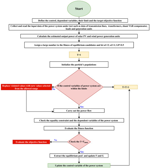
Figure 1. Flowchart of implementation of EO to solve OPF problem.

• Define the control and dependent variables and their limits, as well as the target objective function defined in Section 2.2 [34].
• Collect and read the input data of the power system under test, such as data of transmission lines, transformers, shunt VAR compensator, loads and generation units.
• Calculate the estimated output power of solar PV and wind power generation units, as defined and explained in Section 3 [34].
• Initialize the particle’s populations [34].
• Assign a large number to the fitness of equilibrium candidates and let a1 = 2; a2 = 1; GP = 0.5 [34].
• Do the main while loop as the following [34]:

  (a)

  While (current iteration (Iter) <maximum number of iteration (Max-iter))

  (b)

  For i=1: particles’ number (n)

  (c)

  Find the fitness value of the $i_{th}$ particle

  • If fitness ($C_i$) <fitness ($C_{eq1}$) then
    Substitute ($C_{eq1}$) with ($C_i$) and fitness ($C_{eq1}$)
    with fitness ($C_i$)
  • Else if fitness ($C_i$) >fitness ($C_{eq1}$) & fitness ($C_i$) <fitness ($C_{eq2}$) then
    Substitute ($C_{eq2}$) with ($C_i$) and fitness ($C_{eq2}$)
    with fitness ($C_i$)
  • Else if fitness ($C_i$) >fitness ($C_{eq1}$) & fitness ($C_i$) >fitness ($C_{eq2}$) & fitness ($C_i$) <fitness ($C_{eq3}$) then
    Substitute ($C_{eq3}$) with ($C_i$) and fitness ($C_{eq3}$)
    with fitness ($C_i$)
  • Else if fitness ($C_i$) >fitness ($C_{eq1}$) & fitness ($C_i$) >fitness ($C_{eq2}$) & fitness ($C_i$) >fitness ($C_{eq3}$) & fitness ($C_i$) <fitness ($C_{eq4}$) then
    Substitute ($C_{eq4}$) with ($C_i$) and fitness ($C_{eq4}$) with fitness ($C_i$)

  (d)

  End (if)

  (e)

  End (for)

• Find the $\overrightarrow{C_{avg}}$ according to Equation (37).
• Construct the equilibrium pool according to Equation (38) [34].
• In case of the current iteration >1, accomplish memory saving [34].
• Assign t according to Equation (39).
• Do the second for loop as following:
  For i=1: particles’ number

  (a)

  Select one candidate from the equilibrium pool randomly.

  (b)

  Create the two random vector ($\lambda$ and r).

  (c)

  Construct F, $GCP$, $G_0$ and G according to the Equations (34) and (42)–(44), respectively [34].

  (d)

  Update the concentration C according to Equation (45)

  End the second for loop.
• Increase the current iteration by one.
• End the main while loop.
• Extract and analyse of the results.

5. Test Systems and Control Parameters of Optimization Methods

5.1. Description of the Test Power Systems

• Test system 1: IEEE 30-bus system
  The IEEE 30-bus system consists of six thermal power generators, as presented in Figure 2. The data about transmission lines, tap changing transformers, AVR compensators, limitations on generators and load voltages, active and reactive power demand are given in [42,43,44]. The general specifications of this system are described in Table 3.
  

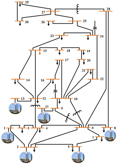  Figure 2. Scenario 1: IEEE 30-bus system.
  Table 3. The general specification of all test power systems.

  	Values and Details
  Characteristics	Test System 1 [42,43,44]	Test System 2	Test System 3	Test System 4
  Buses	30	30	30	30
  Transmission Lines	41	41	41	41
  Limitation on generator voltage	[0.9–1.1]	[0.9–1.1]	[0.9–1.1]	[0.9–1.1]
  Limitation on load voltage	[0.95–1.1]	[0.95–1.1]	[0.95–1.1]	[0.95–1.1]
  Thermal power generators	6	3	3	3
  Wind power plants	0	2	0	5
  Solar power plants	0	3	5	0
  Shunt VAR compensation	9	9	9	9
  Transformer with tap ratio	4	4	4	4
  Control Variables	24	28	28	28
  Active and Reactive power demand	283.4 MW, 126.2 Mvar	283.4 MW, 126.2 Mvar	283.4 MW, 126.2 Mvar	283.4 MW, 126.2 Mvar

• Test system 2: Hybrid wind and solar PV integrated IEEE 30-bus system
  This modified test power system is simulated to show its behavior in the presence of both wind and solar PV power generating units, as depicted in Figure 3. The IEEE 30-bus system has been modified by replacing the thermal power generating units at buses 5, 11, and 13 with wind generator at bus 11 and solar PV at buses 5 and 13. In addition, the new solar PV and wind power generators are constructed at bus 24, and 30, respectively. The objective functions defined in Section 2.2 are modified by adding the output power of solar PV plants ($P_s(G)$) and the output power of wind plants ($P_w(v)$) given in Section 3. Case 3 and case 5 described in Section 2.2 are modified by adding the total cost of solar PV plants ($C_T^{PV}$) and the total cost of wind plants ($C_T^w$) defined in Section 3. The specification of this hybrid power system is given in Table 3. The data of wind and solar PV plants are described in Table 4 and Table 5, respectively.
  

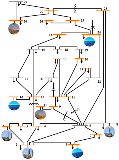  Figure 3. Hybrid wind and solar PV integrated IEEE 30-bus system.
  Table 4. Data of wind power plant for Test system 2.

  Unit	Bus	No. of Turbines	${\mathit{P}}_{\mathit{wr}}$ [MW]	k	c	${\mathit{g}}_{\mathit{i}}$ [$/MWH]	${\mathit{K}}_{\mathit{Rw},\mathit{i}}$ [$/MWH]	${\mathit{K}}_{\mathit{Pw},\mathit{i}}$ [$/MWH]	${\mathit{v}}_{\mathit{in}}$ [m/s]	${\mathit{v}}_{\mathit{out}}$ [m/s]	${\mathit{v}}_{\mathit{r}}$ [m/s]
  1	11	12	2	2	9	1.7	2.8	1.7	4	25	13
  2	30	12	2	2	10	1.7	2.8	1.7	4	25	13

  Table 5. Data of solar power plant for Test system 2.

  Unit	Bus	${\mathit{P}}_{\mathit{sr}}$ [MW]	${\mathit{G}}_{\mathit{std}}$ [W/m${}^2$]	${\mathit{R}}_{\mathit{c}}$ [W/m${}^2$]	$\mathit{\mu }$	$\mathit{\sigma }$	${\mathit{h}}_{\mathit{k}}$ [$/MWh]	${\mathit{K}}_{\mathit{Ps},\mathit{k}}$ [$/MWh]	${\mathit{K}}_{\mathit{Rs},\mathit{k}}$ [$/MWh]
  1	5	24	800	170	6	0.6	1.55	3.2	1.30
  2	13	30	800	170	6	0.6	1.45	3.1	1.45
  3	30	30	800	200	6	0.6	1.60	3.0	1.30

• Test system 3: Solar PV integrated IEEE 30-bus system
  This system is modified by locating solar PV generators at buses 5, 11, and 13 instead of the thermal power generators. Furthermore, two new solar power generation units are installed at buses 24, and 30, as shown in Figure 4. The objective funtions defined in Section 2.2 are modified by adding the output power of solar PV plants ($P_s(G)$) given in Section 3. Case 3 and case 5 described in Section 2.2 are modified by adding the total cost of solar PV plants ($C_T^{PV}$) defined in Section 3. The general data of this system and solar PV plants are presented in Table 3 and Table 6, respectively.
  

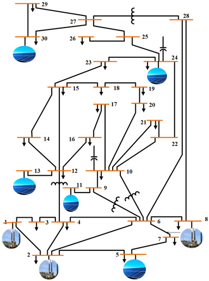  Figure 4. Solar PV integrated IEEE 30-bus system.
  Table 6. Data of solar power plant for Test system 3.

  Unit	Bus	${\mathit{P}}_{\mathit{sr}}$ [MW]	${\mathit{G}}_{\mathit{std}}$ [W/m${}^2$]	${\mathit{R}}_{\mathit{c}}$ [W/m${}^2$]	$\mathit{\mu }$	$\mathit{\sigma }$	${\mathit{h}}_{\mathit{k}}$ [$/MWh]	${\mathit{K}}_{\mathit{Ps},\mathit{k}}$ [$/MWh]	${\mathit{K}}_{\mathit{Rs},\mathit{k}}$ [$/MWh]
  1	5	24	800	170	6	0.6	1.55	3.2	1.30
  2	11	24	800	200	6	0.6	1.45	2.8	1.30
  3	13	24	800	170	6	0.6	1.60	3.1	1.45
  4	24	30	800	170	6	0.6	1.60	3.0	1.30
  5	30	30	800	200	6	0.6	1.60	3.0	1.30

• Test system 4: wind integrated IEEE 30-bus system
  In this system, the IEEE 30-bus system is modified by replacing the thermal power generating units at buses 5, 11, and 13 with wind power generators. Moreover, two new wind generators have been added at buses 24, and 30, as seen in Figure 5. The objective functions defined in Section 2.2 is modified by adding the output power of wind plants ($P_w(v)$) given in Section 3. Case 3 and case 5 described in Section 2.2 are modified by adding the total cost of wind plants ($C_T^w$) defined in Section 3. The general specifications of this system and the data of wind power plants are given in Table 3 and Table 7, respectively.
  

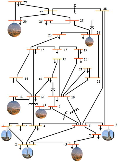  Figure 5. Wind integrated IEEE 30-bus system.
  Table 7. Data of wind power plant for Test system 4.

  Unit	Bus	No. of Turbines	${\mathit{P}}_{\mathit{wr}}$ [MW]	k	c	${\mathit{g}}_{\mathit{i}}$ [$/MWH]	${\mathit{K}}_{\mathit{Rw},\mathit{i}}$ [$/MWH]	${\mathit{K}}_{\mathit{Pw},\mathit{i}}$ [$/MWH]	${\mathit{v}}_{\mathit{in}}$ [m/s]	${\mathit{v}}_{\mathit{out}}$ [m/s]	${\mathit{v}}_{\mathit{r}}$ [m/s]
  1	5	12	2	2	9	1.65	2.6	1.5	4	25	13
  2	11	12	2	2	10	1.60	2.6	1.5	4	25	13
  3	13	12	2	2	9	1.60	2.6	1.5	4	25	13
  4	24	15	2	2	10	1.65	2.6	1.5	4	25	13
  5	30	15	2	2	9	1.70	2.6	1.5	4	25	13

5.2. Control Parameters of Optimization Methods

The number of iterations, population size, testing ranges and other parameters of the optimization methods are given in Table 8.

Table 8. Control parameters values for optimization methods.

Algorithm	Parameters	Values
MPSO [45]	Inertia coefficient (w)	decreasing linearly from 0.9 to 0.4
	Number of search agents	50
	Maximum number of iteration	100
	Udapting factor (C1,C2)	Described in [45]
	Acceleration coefficient (c1,c2)	c1 = 1, c2 = 2
TLBO [46]	Teaching factor	Selected randomly [1,2]
	Population size	50
	Maximum number of iteration	100
TACPSO [45]	Inertia coefficient (w)	decreasing linearly from 0.9 to 0.4
	Number of search agents	50
	Maximum number of iteration	100
	Udapting factor (C1,C2)	Described in [45]
	Acceleration coefficient (c1,c2)	c1 = 1, c2 = 2
MFO [47]	Population size	50
	Maximum number of iteration	100
	Shape constant (b)	1
AGPSO 1 [45]	Inertia coefficient (w)	decreasing linearly from 0.9 to 0.4
	Number of search agents	50
	Maximum number of iteration	100
	Udapting factor (C1,C2)	Described in [45]
	Acceleration coefficient (c1,c2)	c1 = 1, c2 = 2
EO [34]	Constant values for controlling exploration ($a_1$)	2
	Constant values for controlling exploitation ($a_2$)	1
	Number of search particles	50
	Maximum number of iteration	100
	Generation probability	0.5

6. Results and Discussion

The performance and effectiveness of the EO are verified for solving OPF problem by carrying out 20 independent test trial runs for all cases discussed in Section 2.2. The EO [34] and other five metaheuristic optimization techniques: MFO [47], TACPSO [45], AGPSO1 [45], TLBO [46] and MPSO [45] have been tested on four power test systems given in Section 5.1. All these optimization techniques are implemented on 2.8-GHz i7 PC with 16 GB of RAM using MATLAB 2017.

6.1. Discussion and Analysis of the Objective Functions of OPF

6.1.1. Minimization of Real Power Loss

The EO [34], TLBO [46], MPSO [45], MFO [47], AGPSO1 [45], and TACPSO [45] algorithms are implemented on the test system 1, test system 2, test system 3, and test system 4 for the minimization of the real power loss as defined in Section 2.2. Figure 6a shows the convergence characteristics of real power loss yielded by the best solution of the EO and other optimization methods for test system 1. It observed that the better convergence characteristic is yielded by the EO. Furthermore, Figure 6b,c display voltage and loading profiles of test system 1 for case 1. It is clear that the EO and other optimization methods obey the voltage limits of buses and loading limits of transmission lines. The results of EO and other techniques for test system 1 are displayed in Table 9. It can be observed that EO achieves the minimum real power loss, but other optimization techniques such as TLBO and MFO have less fuel cost at 967.24 $/h and 967.44 $/h, respectively. Furthermore, other techniques have less voltage deviations at minimization this objective function. However, it is clear that the loading of transmission lines for EO is healthy and less than other methods.

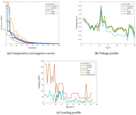
Figure 6. Comparative convergence, voltage and loading profiles for case 1 for all test systems.

Table 9. Results of EO and other methods of case 1 for Test system 1.

	MFO	TACPSO	AGPSO1	TLBO	EO	MPSO
$VD$ (p.u.)	0.867649	0.898003	0.898362	0.87350728	0.917249	0.679794
$FC$ ($/h)	967.4482	967.6206	967.6485	967.2492825	967.5865	967.7676
$P_{loss}$ (MW)	3.124412	3.100891	3.094156	3.108417583	3.087342	3.144079
E (ton/h)	0.207299	0.207259	0.207266	0.207286164	0.207268	0.207273
$f_o$	3.124412	3.100891	3.094156	3.108417583	3.087342	3.144079
$Improvement (\%)$	1.18	0.43	0.22	0.68	-	1.81

The loss and loading profiles using EO for all test systems are given in Figure 7. The optimal (best) results yielded by the EO method for the test system 1, test system 2, test system 3, and test system 4 are tabulated in Table 10. From Figure 7 and Table 10, it is seen that the losses of test system 2, test system 3, and test system 4 reduced by 23.6%, 31.52%, and 33.32%, respectively, compared to test system 1. Additionally, it can be seen that the contribution of power generation of Test system 2 from wind, solar PV and thermal power generation are 15.05%, 33.01%, and 51.93%, respectively. With respect to Test system 3, the contribution of power generation from solar PV and thermal power are 53.33% and 46.66%, respectively. Besides, the wind power plants of Test system 4 contributes 52.35% of the total power generation.

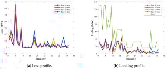
Figure 7. Loss and loading Profiles of case 1 for all test systems using EO.

Table 10. Optimal settings of dependent and control variables for case 1 for all test systems using EO.

Parameters	Min	Max	Test System 1	Test System 2	Test System 3	Test System 4
PG2 (MW)	20	80	79.9983006	72.14028714	48.22886744	51.07651611
PG5 (MW)	15	50	49.9982627	49.99945385	49.97347066	49.98470056
PG8 (MW)	10	35	34.99453958	26.20234283	34.77838714	34.92764479
PG11 (MW)	10	30	29.99984469	29.42347144	29.97517159	29.67713532
PG13 (MW)	10	40	39.99027741	25.72695297	29.69711674	39.69895071
PG24 (MW)	10	30		18.61010237	27.4148297	15.73782289
PG30 (MW)	10	40		13.58641689	15.23102984	14.35575851
V1 (p.u.)	0.95	1.1	1.061430345	1.033582214	1.037749499	1.056224426
V2 (p.u.)	0.95	1.1	1.057379791	1.027683624	1.032739079	1.051241045
V5 (p.u.)	0.95	1.1	1.037622078	1.003632229	1.013755431	1.032812731
V8 (p.u.)	0.95	1.1	1.044007621	1.015022765	1.02707043	1.045463882
V11 (p.u.)	0.95	1.1	1.073279794	1.063216144	0.999050197	1.042867188
V13 (p.u.)	0.95	1.1	1.051619936	1.034701938	1.044856898	1.020563172
V24 (p.u.)	0.95	1.1		1.024480465	1.009002895	1.020352939
V30 (p.u.)	0.95	1.1		1.022453184	1.018925985	1.040981535
QC10 (MVAr)	0	5	4.287709826	4.782286758	2.62406261	3.612693403
QC12 (MVAr)	0	5	2.093601675	0.000803534	0.986423834	2.416935212
QC15 (MVAr)	0	5	3.996488379	1.898614523	0.206692775	3.600783886
QC17 (MVAr)	0	5	4.136235738	4.356883849	2.716911629	0.342465282
QC20 (MVAr)	0	5	4.495134896	3.354513668	4.692404829	3.296807199
QC21 (MVAr)	0	5	5.000000000	0.046094293	2.038284465	0.872744865
QC23 (MVAr)	0	5	3.197386977	4.967912056	4.957773966	4.740324068
QC24 (MVAr)	0	5	4.806462479	4.536993047	3.79952116	3.698494945
QC29 (MVAr)	0	5	2.461175597	0.21865228	4.63994E−05	3.927880442
T11 (p.u.)	0.9	1.1	1.055740955	1.015687471	1.020034326	1.0962353
T12 (p.u.)	0.9	1.1	0.924042761	0.951998195	0.957069803	0.900424717
T15 (p.u.)	0.9	1.1	0.988530694	0.989254661	1.094558386	0.991494831
T36 (p.u.)	0.9	1.1	0.975749345	0.977273155	1.010207101	1.010623787
PG1 (MW)	50	200	51.50611659	50.08572807	50.22954768	50.01396753
QG1 (MVAr)	−20	150	−5.485983591	−1.712627012	−9.408754457	−4.363894439
QG2 (MVAr)	−20	60	7.574416698	7.129014137	3.920290677	9.504062082
QG5 (MVAr)	−15	62.5	21.13271229	17.01446382	19.68757038	20.6489489
QG8 (MVAr)	−15	48	26.41312254	26.16274206	28.52016815	33.06577869
QG11 (MVAr)	−10	40	19.21231862	19.38101083	0.13383456	18.93870787
QG13 (MVAr)	−15	44	2.247530335	8.029799729	33.49981989	−2.320248965
QG24 (MVAr)	−15	44		3.105401958	3.720374455	2.56415683
QG 30 (MVAr)	−15	44		0.296246809	2.993820748	1.368798025
$VD$ (p.u.)			0.917249187	0.367181831	0.252949566	0.482190403
$FC$ ($/h)			967.5864625	417.7815499	358.1435956	368.1354088
$P_{loss}$ (MW)			3.087341565	2.374755583	2.128420834	2.072496662
E (ton/h)			0.20726839	0.09655031	0.09111361	0.091202895
$TC$ ($/h)				863.2203104	823.476285	867.8385329
$C_T^W$ ($/h)				141.4837171		499.7031241
$C_T^{PV}$ ($/h)				303.9550435	465.3326895
$f_o$ (MW)			3.087341565	2.374755583	2.128420834	2.072496662

The statistical results (the best, the worst, the mean, and the standard deviation) of the real power loss for the EO and other optimization techniques are given in Table 11. As shown in Table 11, the minimum best, standard deviation, and mean are resulted from the EO.

Table 11. Summary of the statistical analysis of case 1 for Test system 1.

	Best	Worst	Mean	Std dev
MFO	3.124412	3.469255	3.313791	0.115148
TACPSO	3.100891	3.495604	3.162984	0.119564
AGPSO1	3.094156	3.558659	3.136808	0.175963
TLBO	3.108418	3.271804	3.200392	0.057571
EO	3.087342	3.131426	3.089549	0.013218
MPSO	3.144079	3.417325	3.202598	0.080901

As expected, the addition and location of the renewable energy resources in the power system have a significant impact on reducing the real power loss.

6.1.2. Emission Index Minimization

In this case, the emission index defined in Section 2.2 was minimized for all test systems. Figure 8 demonstrates the convergence characteristics, loss profiles, and loading profiles for emission minimization using EO and other methods. It can be noticed from Figure 8a that the EO has the smoothest and speediest convergence curves in comparing with other techniques, as well as Figure 8b,c showing that there is no violation in the voltage limits of buses and loading limits of transmission lines. As we can see from Table 13 and Figure 8c that EO can achieve the lowest real power loss and the lowest loading of the transmission lines while minimizing this objective function, but other optimization methods can obtain less voltage deviations in comparison to EO.

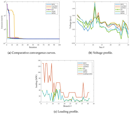
Figure 8. Comparative convergence, voltage and loading Profiles for case 2 for all test systems.

The best (optimal) results obtained using the EO for all test systems for case 2 are shown in Table 12. As we can see from Figure 9 and Table 12 that emission index reduced by 55.54% for test system 2, test system 3, and test system 4 compared to test system 1. In this case, the contribution of power generation from wind power plants for Test system 2 and Test system 4 are 12.25% and 54.12% of the total generation, respectively. In addition, the contribution of power generation from solar PV for Test system 2 and Test system 3 are 41.69% and 53.93% of the total generation, respectively.

Table 12. Optimal settings of dependent and control variables for case 2 for all test systems using EO.

Parameters	Min	Max	Test System 1	Test System 2	Test System 3	Test System 4
PG2 (MW)	20	80	67.52765352	47.15393481	46.93784062	46.74579811
PG5 (MW)	15	50	49.99976843	49.99997692	48.55695793	49.63943974
PG8 (MW)	10	35	34.99979715	34.99785564	35.00000000	34.99981323
PG11 (MW)	10	30	30.00000000	13.08937369	24.11263394	28.93951933
PG13 (MW)	10	40	39.99994042	39.97364116	38.90979918	31.15977654
PG24 (MW)	10	30		29.67649489	20.72363213	13.68967898
PG30 (MW)	10	40		22.06349364	22.1793691	32.00183302
V1 (p.u.)	0.95	1.1	1.061391900	1.035577033	1.017785294	1.007633877
V2 (p.u.)	0.95	1.1	1.055299891	1.03014784	1.009596473	0.99225379
V5 (p.u.)	0.95	1.1	1.036061646	0.975474909	0.982885915	0.966515297
V8 (p.u.)	0.95	1.1	1.042336524	0.994262522	0.996877809	0.970873143
V11 (p.u.)	0.95	1.1	1.056098162	0.99155371	1.066472978	1.018197794
V13 (p.u.)	0.95	1.1	1.061630874	1.045591502	1.053301428	0.990382535
V24 (p.u.)	0.95	1.1		0.994310052	1.023161602	1.006430427
V30 (p.u.)	0.95	1.1		0.976743321	0.962066536	0.995194145
QC10 (MVAr)	0	5	4.194820255	0.691891638	0.00000000	2.28917862
QC12 (MVAr)	0	5	0.527663733	3.89808945	4.781805725	0.003693677
QC15 (MVAr)	0	5	4.925786364	0.093781976	4.681393138	3.767863825
QC17 (MVAr)	0	5	4.982842903	2.766984513	4.998326488	4.887538377
QC20 (MVAr)	0	5	4.671024822	4.426843395	4.610963598	5.000000000
QC21 (MVAr)	0	5	4.976075346	1.329009086	4.940763823	2.759967479
QC23 (MVAr)	0	5	2.74762835	3.54838243	0.002439547	4.271161763
QC24 (MVAr)	0	5	4.992557282	0.606928317	0.970384621	2.50397663
QC29 (MVAr)	0	5	2.088379542	4.949034272	0.000438444	2.957731038
T11 (p.u.)	0.9	1.1	1.045594251	0.951879814	0.938502294	0.940072546
T12 (p.u.)	0.9	1.1	0.921878284	0.962206441	1.096587454	0.919312335
T15 (p.u.)	0.9	1.1	1.00248085	1.099174642	1.018026147	1.023627655
T36 (p.u.)	0.9	1.1	0.972355171	0.92579926	1.099689643	1.060629423
PG1 (MW)	50	200	64.09434175	50.00003511	50.00023516	50.00000501
QG1 (MVAr)	−20	150	−5.544691231	0.054641352	−1.33241509	18.58616272
QG2 (MVAr)	−20	60	6.45002148	47.44923402	4.202024706	1.97952536
QG5 (MVAr)	−15	62.5	21.67156016	−1.442938766	13.43474762	19.83503047
QG8 (MVAr)	−15	48	27.29675405	23.11453954	7.583267029	12.95707181
QG11 (MVAr)	−10	40	11.72500454	−6.137543909	13.66528344	1.654000716
QG13 (MVAr)	−15	44	9.840166661	39.23629311	21.68524583	6.151027816
QG24 (MVAr)	−15	44		1.089772208	24.29742231	20.10756016
QG 30 (MVAr)	−15	44		−13.49116551	0.162345045	0.721702425
$VD$ (p.u.)			0.90040310	0.298468513	0.404641642	0.391340877
$FC$($/h)			944.2808599	354.7638857	354.038595	353.3864113
$P_{loss}$ (MW)			3.22150126	3.554805885	3.020468191	3.775864192
E (ton/h)			0.204818699	0.091061921	0.091060623	0.091060048
$TC$ ($/h)				877.5739313	865.4758094	867.8663197
$C_T^W$ ($/h)				108.3986993		514.4799085
$C_T^{PV}$ ($/h)				414.4113463	511.4372144
$f_o$ (ton/h)			0.204818699	0.091061921	0.091060623	0.091060048

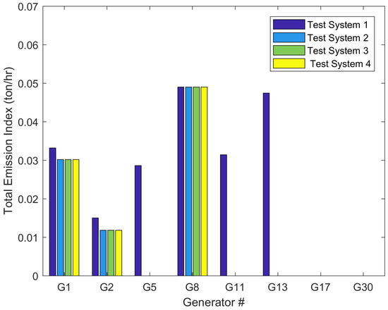
Figure 9. Total Emission index (ton/hr) of case 2 for all test systems using EO.

Table 13 presents the results of the EO and other methods for test system 1 with the minimization of emission index. For example, the objective function of case 2 for EO was 0.204819 ton/h compared to 0.204862 ton/h and 0.204885 ton/h for MFO [47] and TLBO [46] algorithms, respectively.

Table 13. Results of EO and other methods of case 2 for Test system 1.

	MFO	TACPSO	AGPSO1	TLBO	EO	MPSO
$VD$ (p.u.)	0.702001	0.856848	0.921129	0.541768425	0.900403	0.661504
$FC$ ($/h)	944.3434	944.6554	944.3977	944.6873755	944.2809	944.4382
$P_{loss}$ (MW)	3.356033	3.286856	3.235581	3.336091467	3.221501	3.267419
E (ton/h)	0.204862	0.204839	0.204823	0.204854728	0.204819	0.204833
$f_o$ (ton/h)	0.204862	0.204839	0.204823	0.204854728	0.204819	0.204833

Table 14 summarizes the statistical results for the present case. It can be found from Table 14 that the EO provides the smallest best, standard deviation, and median than other methods.

Table 14. Summary of the statistical analysis of case 2 for Test system 1.

	Best	Worst	Mean	Std Dev
MFO	0.204862	0.204997	0.20495	4.15 × 10${}^{-5}$
TACPSO	0.204839	0.205089	0.204943	9.14 × 10${}^{-5}$
AGPSO1	0.204823	0.204999	0.204921	5.14 × 10${}^{-5}$
TLBO	0.204855	0.204931	0.204892	2.43 × 10${}^{-5}$
EO	0.204819	0.204878	0.204834	1.78 × 10${}^{-5}$
MPSO	0.204833	0.20497	0.204934	5.44 × 10${}^{-5}$

6.1.3. Minimization of the Total Cost of Generating Units

The comparative convergence characteristics, loading profiles, and loss profiles for test system 1 for the EO and other optimization techniques are presented in Figure 10. As observed in Figure 10, the voltage and loading profiles are kept within the acceptable ranges and the EO gives the best convergence characteristics compared to other methods. The optimal results of the EO and other techniques for test system 1 are summarized in Table 15. From Table 15, the EO leads to 800.4486 $/h total cost of generators which is better than the total cost obtained by the other compared methods. From Figure 10b,c, it can be found that even though EO can obtain the minimum value of the total cost of power generation, the loading of the transmission lines is more than other methods and voltage deviation of EO is higher than other optimization techniques.

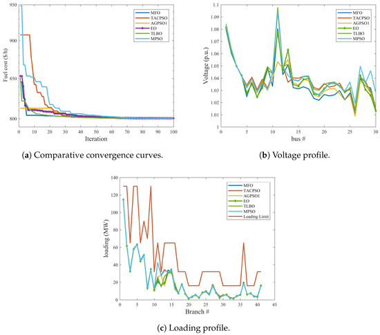
Figure 10. Comparative convergence, voltage and loading Profiles for case 3 for all test systems.

Table 15. Results of EO and other methods of case 3 for Test system 1.

	MFO	TACPSO	AGPSO1	TLBO	EO	MPSO
$VD$ (p.u.)	0.740965	0.845878	0.761669	0.811019872	0.865075	0.877139
$FC$ ($/h)	800.8283	800.5201	800.5595	800.616176	800.4486	800.5346
$P_{loss}$ (MW)	9.134902	9.02898	9.040104	8.97569702	9.041464	9.059254
E (ton/h)	0.366492	0.366315	0.365967	0.363482104	0.367478	0.366949
$f_o$ ($/h)	800.8283	800.5201	800.5595	800.616176	800.4486	800.5346

The statistical results yielded by the EO and other optimization techniques are given in Table 16.

Table 16. Summary of the statistical analysis of case 3 for Test system 1.

	Best	Worst	Mean	Std Dev
MFO	800.8283	802.8078	801.5102	0.72899
TACPSO	800.5201	804.0448	800.6766	1.305504
AGPSO1	800.5595	802.1145	800.7023	0.453581
TLBO	800.6162	802.225	800.8366	0.471362
EO	800.4486	800.646	800.4793	0.057894
MPSO	800.5346	804.6442	801.1155	1.810857

From Table 17 and Figure 11, it can be observed that the total cost of generating units for test system 2, test system 3, and test system 4 declined by 3.54%, 3.47%, and 2.91%, respectively, compared to test system 1. In this case, as shown in Table 17; the contribution of power generation from wind power plants for Test system 2 and Test system 4 are 9.58% and 35.68% of the total generation, respectively. Moreover, the contribution of power generation from solar PV for Test system 2 and Test system 3 are 21.33% and 41.17% of the total generation, respectively.

Table 17. Optimal settings of dependent and control variables for case 3 for all test systems using EO.

Parameters	Min	Max	Test System 1	Test System 2	Test System 3	Test System 4
PG2 (MW)	20	80	48.74605575	45.18712121	21.21838812	38.17119779
PG5 (MW)	15	50	21.4315437	15.00195728	15.40668673	19.095538
PG8 (MW)	10	35	21.18353338	29.97018297	15.60913424	10.08641797
PG11 (MW)	10	30	11.52952165	13.07275916	29.402226	20.7452611
PG13 (MW)	10	40	12.0107829	19.71387022	30.51540057	17.9328134
PG24 (MW)	10	30		27.19702311	26.3304831	25.32965431
PG30 (MW)	10	40		14.74139467	17.72178713	20.28023584
V1 (p.u.)	0.95	1.1	1.081191705	1.022713246	1.02314065	1.059255936
V2 (p.u.)	0.95	1.1	1.063110135	1.006065736	1.008766945	1.043719467
V5 (p.u.)	0.95	1.1	1.032684857	0.956733982	0.961917138	1.009460201
V8 (p.u.)	0.95	1.1	1.036543249	0.994159517	0.985269141	1.02095678
V11 (p.u.)	0.95	1.1	1.097591909	1.012587735	1.049992902	1.0845661
V13 (p.u.)	0.95	1.1	1.051244633	1.054638289	1.011514979	1.046208927
V24 (p.u.)	0.95	1.1		1.035583887	1.011800496	1.043496784
V30 (p.u.)	0.95	1.1		0.950000000	0.996591531	1.048407181
QC10 (MVAr)	0	5	2.971616423	3.739491269	4.902790106	0.325756054
QC12 (MVAr)	0	5	0.655177618	4.809891924	1.662706176	3.06145818
QC15 (MVAr)	0	5	3.197516308	0.002648509	0.249875162	3.301750446
QC17 (MVAr)	0	5	4.723716655	3.279961844	1.827574807	1.707154585
QC20 (MVAr)	0	5	3.650622268	0.917150962	1.107119341	0.418013886
QC21 (MVAr)	0	5	5.000000000	4.948708899	2.08610321	4.893042007
QC23 (MVAr)	0	5	2.498554056	4.535914953	4.240774401	3.58924067
QC24 (MVAr)	0	5	4.985418463	5.000000000	0.00000000	1.169769378
QC29 (MVAr)	0	5	2.584313587	4.144114834	4.95463484	1.500067393
T11 (p.u.)	0.9	1.1	1.027284076	1.048412041	1.099843892	0.985023037
T12 (p.u.)	0.9	1.1	0.971275895	0.90000000	0.922169184	0.989956238
T15 (p.u.)	0.9	1.1	0.972373363	1.002944153	1.006664961	0.991751478
T36 (p.u.)	0.9	1.1	0.9815263	1.059841992	0.944073975	0.971316876
PG1 (MW)	50	200	177.5400261	125.374001	133.7249716	138.0708394
QG1 (MVAr)	−20	150	−0.570024945	−0.833938199	−5.669301771	−1.647701957
QG2 (MVAr)	−20	60	19.80925666	13.30674022	30.0465083	18.91158888
QG5 (MVAr)	−15	62.5	25.58480054	6.160576051	11.07617293	21.00268292
QG8 (MVAr)	−15	48	23.28431397	23.75265502	14.5584729	21.65678972
QG11 (MVAr)	−10	40	25.55139519	8.157153402	35.09222447	19.52230631
QG13 (MVAr)	−15	44	1.335643081	21.55072062	12.13070192	7.287213883
QG24 (MVAr)	−15	44		22.34214251	15.27252587	8.101017671
QG 30 (MVAr)	−15	44		−5.331414964	−8.278410983	−1.403218975
$VD$ (p.u.)			0.865074691	0.312619858	0.288839815	0.653856503
$FC$ ($/h)			800.4486031	529.3973749	432.2815387	473.5571537
$P_{loss}$ (MW)			9.041463508	6.858309749	6.529077621	6.311958209
E (ton/h)			0.367478227	0.141650437	0.159248156	0.163097259
$TC$ ($/h)				772.2465456	772.7810970	777.3121394
$C_T^W$ ($/h)				85.46692162		303.7549857
$C_T^{PV}$ ($/h)				157.3822491	340.4995583
$f_o$ ($/h)			800.4486031	772.2465456	772.7810970	777.3121394

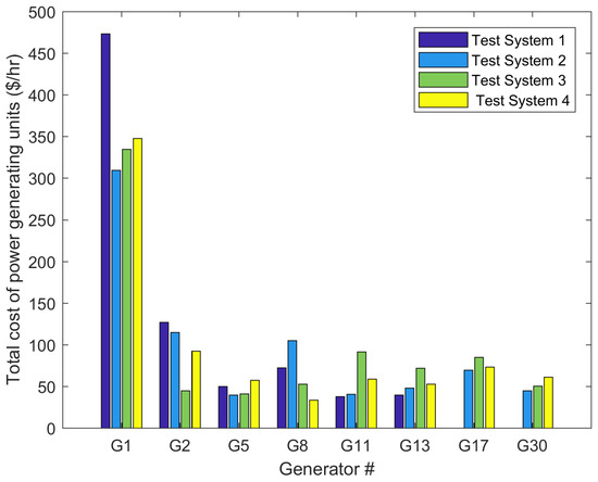
Figure 11. Total cost of generating units of case 3 for all test systems using EO.

6.1.4. Voltage Deviation Minimization

Figure 12 demonstrates the voltage profiles for all test systems for this case using EO. The optimal solution obtained by EO for test system 1, test system 2, test system 3, and test system 4 are tabulated in Table 18. As shown in Figure 12 and Table 18, the presence of the renewable energy resources improves the voltage profiles and reduced the voltage deviation for test system 2, test system 3, and test system 4 by 22.46%, 37.39%, and 29.61%, respectively, compared to test system 1. Besides, it can be observed that the power generation contribution of Test system 2 from wind, solar PV and thermal power generation are 17.57%, 17.87%, and 64.54%, respectively. With respect to Test system 3, the contribution of power generation from solar PV and thermal power are 34.69% and 65.30%, respectively. Moreover, the wind power plants of Test system 4 contribute 55.34% of the total power generation.

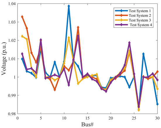
Figure 12. Voltage profiles of case 4 for all test systems using EO.

Table 18. Optimal settings of dependent and control variables for case 4 for all test systems using EO.

Parameters	Min	Max	Test System 1	Test System 2	Test System 3	Test System 4
PG2 (MW)	20	80	70.18121441	35.84850999	73.22346542	42.82238053
PG5 (MW)	15	50	25.52703119	20.27116158	33.56379457	47.02961201
PG8 (MW)	10	35	28.87890546	17.61889372	18.04097353	33.85695266
PG11 (MW)	10	30	29.30401557	24.63092203	10.13966121	14.67013887
PG13 (MW)	10	40	27.92172576	15.28698582	21.57955174	39.93831108
PG24 (MW)	10	30		16.34156919	10.07569951	28.44997135
PG30 (MW)	10	40		26.43024961	24.9797807	28.73744876
V1 (p.u.)	0.95	1.1	1.009811989	1.032801388	1.022207169	1.012647301
V2 (p.u.)	0.95	1.1	1.003153500	1.026505843	1.020581934	1.004121334
V5 (p.u.)	0.95	1.1	1.015213206	1.016105476	1.019877057	1.020275353
V8 (p.u.)	0.95	1.1	1.008124785	0.993094249	0.998231049	1.001227396
V11 (p.u.)	0.95	1.1	1.038640051	1.003641057	1.02134836	0.99563608
V13 (p.u.)	0.95	1.1	1.005894818	1.02703208	0.996453698	1.022325949
V24 (p.u.)	0.95	1.1		1.013528762	1.014235434	1.018656779
V30 (p.u.)	0.95	1.1		1.002929877	0.993533496	0.998414844
QC10 (MVAr)	0	5	4.999434200	1.057601365	4.449085771	1.224696754
QC12 (MVAr)	0	5	4.602398118	2.55410853	4.99999823	2.663316679
QC15 (MVAr)	0	5	4.960424711	4.999607248	1.610176653	3.415934203
QC17 (MVAr)	0	5	0.01181544	0.217347144	1.996228043	0.019033266
QC20 (MVAr)	0	5	4.996883927	4.92956648	4.978309396	4.994054795
QC21 (MVAr)	0	5	4.956429831	1.646590977	0.034134918	4.819904248
QC23 (MVAr)	0	5	4.972309922	0.427048793	1.956957345	1.039869954
QC24 (MVAr)	0	5	4.980435681	2.406207968	4.614781826	0.613094925
QC29 (MVAr)	0	5	2.520824595	1.71349761	3.890942901	3.740081954
T11 (p.u.)	0.9	1.1	1.056622635	1.012874303	1.035801681	1.002332018
T12 (p.u.)	0.9	1.1	0.901402975	0.900602964	0.902285005	0.901103808
T15 (p.u.)	0.9	1.1	0.981060937	1.013218403	0.960787866	0.998733169
T36 (p.u.)	0.9	1.1	0.966944023	0.987755959	0.989855906	0.98143194
PG1 (MW)	50	200	108.1160533	133.9296827	97.60688393	51.45175998
QG1 (MVAr)	−20	150	−19.10239902	−19.59757178	−19.11821266	−0.518817877
QG2 (MVAr)	−20	60	−14.85253038	31.85856685	18.90601653	−16.64972076
QG5 (MVAr)	−15	62.5	57.49581183	49.60698522	51.42002978	56.50571855
QG8 (MVAr)	−15	48	45.23093447	11.80532985	26.14354452	31.44056819
QG11 (MVAr)	−10	40	20.12674964	2.380585374	10.62092072	−1.914317997
QG13 (MVAr)	−15	44	−1.74441538	13.80317636	−8.465359993	10.55389137
QG24 (MVAr)	−15	44		14.86630972	15.99035449	13.88576475
QG 30 (MVAr)	−15	44		−4.888937122	−7.68659143	−7.960636408
$VD$ (p.u.)			0.088397534	0.08005165	0.064632335	0.07266919
$FC$ ($/h)			848.7795548	480.1984844	514.2584395	339.455916
$P_{loss}$ (MW)			6.528945889	6.957974748	5.809810669	3.556575273
E (ton/h)			0.240505607	0.155665569	0.119726864	0.091393798
$TC$ ($/h)				787.9483007	810.1863986	861.8303756
$C_T^W$ ($/h)				164.0403370		522.3744597
$C_T^{PV}$ ($/h)				143.7094792	295.9279591
$f_o$ (p.u.)			0.088397534	0.080051650	0.064632335	0.07266919

It is clear from Table 19; the minimum best, standard deviation, and median are obtained by the EO.

Table 19. Summary of the statistical analysis of case 4 for Test system 1.

	Best	Worst	Mean	Std Dev
MFO	0.100862	0.137899	0.117452	0.011555
TACPSO	0.092725	0.177792	0.116202	0.025827
AGPSO1	0.102816	0.144276	0.131944	0.015650
TLBO	0.103244	0.152343	0.112717	0.015185
EO	0.088398	0.097568	0.092814	0.002809
MPSO	0.093414	0.202628	0.124612	0.038641

From Figure 13, the voltage and loading profiles for this case for all optimization methods obey the constraints of voltages at load buses and transmission line loading. It can also be observed that the EO convergence characteristic outperforms the convergence characteristics of other methods. The results of EO and other methods for test system 1 are given in Table 20. From Figure 13b,c and Table 20, it can be seen that EO achieves the minimum emission index while minimizing the objective function of voltage deviation. In addition, EO and MFO can obtain the lowest real power loss at 6.528 MW and 5.965 MW, respectively. Nevertheless, MPSO, TLBO, TACPSO, and ACPSO1 obtain lower fuel cost in comparison to EO.

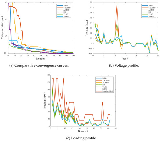
Figure 13. Comparative convergence, voltage and loading profiles for case 4 for all test systems.

Table 20. Results of EO and other methods of case 4 for Test system 1.

	MFO	TACPSO	AGPSO1	TLBO	EO	MPSO
$VD$ (p.u.)	0.100862	0.092725	0.102816	0.103243	0.088398	0.093414
$FC$ ($/h)	901.7397	852.0642	834.1079	829.58791	848.7796	841.3429
$P_{loss}$ (MW)	5.965677	9.980964	7.492151	8.391654	6.528946	7.564352
E (ton/h)	0.248497	0.359732	0.273799	0.337325	0.240506	0.275282
$f_o$ (p.u.)	0.100862	0.092725	0.102816	0.103243	0.088398	0.093414

6.1.5. Case 5: Minimization of the Total Cost of the Generating Units, Voltage Deviation, Real Power Loss, and Emission Index

It is clear from Figure 14 that the EO has the best convergence characteristics compared to the other optimization algorithms and the voltage and loading profiles for all algorithm ranges within the allowable limits. The results of EO and other methods for test system 1 of this case are shown in Table 21. It is clear from Figure 14b,c and Table 21 that while EO achieves the minimum value of voltage deviation and fuel cost in comparison to other methods, other optimization techniques obtain lower values of emission index and real power loss than EO.

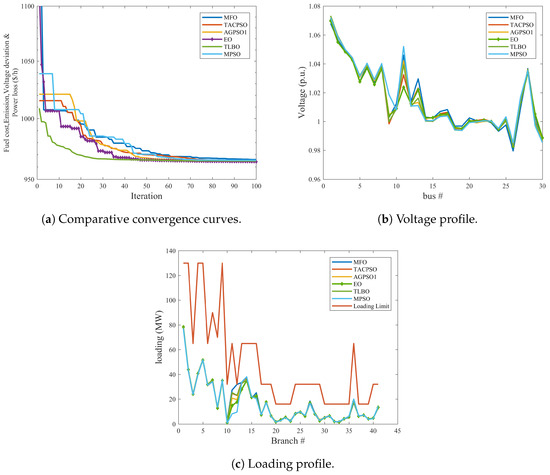
Figure 14. Comparative convergence, voltage and loading profiles for case 5 for all Test system 1.

Table 21. Results of EO and other methods of case 5 for Test system 1.

	MFO	TACPSO	AGPSO1	TLBO	EO	MPSO
$VD$ (p.u.)	0.312222	0.301092	0.2979	0.292001838	0.291525	0.315655
$FC$ ($/h)	832.131	833.4427	831.8455	831.251448	829.9924	833.2358
$P_{loss}$ (MW)	5.569804	5.471244	5.542919	5.575077257	5.604236	5.490564
E (ton/h)	0.250434	0.249973	0.251339	0.252691258	0.253454	0.249919
$f_o$ ($/h)	965.9816	964.8825	964.8211	964.8363202	964.2232	965.4054

The statistical analysis of the EO and other methods for test system 1 is given in Table 22. As shown in the table, the EO gives the minimum best, median and standard deviation.

Table 22. Summary of the statistical analysis of case 5 for Test system 1.

	Best	Worst	Mean	Std dev
MFO	965.9816	970.7178	968.0071	1.616872
TACPSO	964.8825	968.5757	965.8415	1.251791
AGPSO1	964.8211	967.8093	965.6185	0.874411
TLBO	964.8363	968.0825	966.0087	1.105687
EO	964.2232	966.3464	964.5618	0.655197
MPSO	965.4054	978.9642	966.4455	4.054598

It is clear from Figure 15 and Table 23 that the objective function for this case for test system 2, test system 3, and test system 4 dropped by 3.90%, 7.77%, and 7.84%, respectively compared to test system 1. It is found from Table 23 that the real power loss for test system 2, test system 3, and test system 4 dropped by 30.94%, 20.75%, and 46.06%, respectively compared to test system 1. It can be noted in Figure 15 that the contribution of power generation from wind for Test system 2 and Test system 4 are 15.67% and 49.37% of the total power generation, respectively. While the solar PV contributes 33.36% and 44.69% of the total power for test system 2 and test system 3, respectively. Moreover, it is observed from Table 23 that emission index for test system 2, test system 3, and test system 4 dropped by 61.24%, 54.91%, and 58.58%, respectively compared to test system 1.

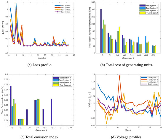
Figure 15. Total cost of generating units, total emission index, voltage and loss profiles of case 5 for all test systems.

Table 23. Optimal settings of dependent and control variables for case 5 for all test systems using EO.

Parameters	Min	Max	Test System 1	Test System 2	Test System 3	Test System 4
PG2 (MW)	20	80	52.34900301	43.76198174	46.85392201	39.04580002
PG5 (MW)	15	50	31.41892625	25.13957863	41.57764325	49.63341394
PG8 (MW)	10	35	34.99720302	28.83722988	15.57308058	21.63539649
PG11 (MW)	10	30	26.95716205	27.72005416	28.54767347	26.5299306
PG13 (MW)	10	40	20.69034077	37.30220041	21.35593529	20.93782021
PG24 (MW)	10	30		33.41823981	19.87429698	27.03669094
PG30 (MW)	10	40		17.31391519	17.29441758	17.27175615
V1 (p.u.)	0.95	1.1	1.073302714	1.024270078	1.031881955	1.034535652
V2 (p.u.)	0.95	1.1	1.05933056	1.012773005	1.014838234	1.023955028
V5 (p.u.)	0.95	1.1	1.031867076	0.991186486	0.965629646	1.002922115
V8 (p.u.)	0.95	1.1	1.039079245	0.991138879	0.993005954	1.010973253
V11 (p.u.)	0.95	1.1	1.039336016	1.100000000	1.038730973	1.039568814
V13 (p.u.)	0.95	1.1	1.016224258	1.023619922	1.047631647	1.010922024
V24 (p.u.)	0.95	1.1		1.027240201	1.008908379	1.012804196
V30 (p.u.)	0.95	1.1		1.026258901	1.033487159	1.015369168
QC10 (MVAr)	0	5	1.42704702	0.24222794	5.00000000	3.367347878
QC12 (MVAr)	0	5	0.114983911	4.465905221	5.00000000	4.957438998
QC15 (MVAr)	0	5	2.71927269	0.00000000	1.436680682	3.38628092
QC17 (MVAr)	0	5	4.777257639	4.971408287	0.00000000	4.999449612
QC20 (MVAr)	0	5	4.891165116	4.864936873	5.00000000	4.836689278
QC21 (MVAr)	0	5	4.917867343	4.114355205	4.252301174	2.729537609
QC23 (MVAr)	0	5	4.944826897	4.912774176	0.00000000	1.224294666
QC24 (MVAr)	0	5	4.999139393	3.383242169	2.790571405	4.901232863
QC29 (MVAr)	0	5	2.36221935	0.622641699	5.00000000	0.478740405
T11 (p.u.)	0.9	1.1	1.098277898	1.041847001	0.996768732	1.070613035
T12 (p.u.)	0.9	1.1	0.937769396	0.906411875	1.061448786	0.920185016
T15 (p.u.)	0.9	1.1	1.02148431	0.939592837	0.983885511	0.995441894
T36 (p.u.)	0.9	1.1	1.002153866	0.991006369	0.904079564	0.993400466
PG1 (MW)	50	200	122.5915999	73.77703	96.76396309	84.33186618
QG1 (MVAr)	−20	150	0.44760914	4.980415704	11.6826979	−1.350997342
QG2 (MVAr)	−20	60	13.45186855	10.12960773	16.17020662	8.009356413
QG5 (MVAr)	−15	62.5	22.96436543	30.2545861	−0.480850004	19.94798351
QG8 (MVAr)	−15	48	25.09929462	4.325252485	25.37843413	24.0097914
QG11 (MVAr)	−10	40	20.42841833	39.34377358	16.58858651	20.9433804
QG13 (MVAr)	−15	44	4.484753294	−4.510415315	19.67801235	1.913484758
QG24 (MVAr)	−15	44		−1.505790029	2.129992746	2.949992903
QG 30 (MVAr)	−15	44		3.138390036	−7.584798837	0.645488754
$VD$ (p.u.)			0.291524702	0.340717958	0.287869453	0.142747756
$FC$ ($/h)			829.9923878	378.7198323	401.6872426	364.5623372
$P_{loss}$ (MW)			5.604235892	3.870229887	4.440932453	3.022674546
E (ton/h)			0.253453881	0.098214148	0.114249163	0.104949647
$TC$ ($/h)				832.9987095	783.9164460	817.6301115
$C_T^W$ ($/h)				144.7990782		453.0677743
$C_T^{PV}$ ($/h)				309.4797989	382.2292034
$f_o$ ($/h)			964.2232199	927.1649129	889.8329526	889.1206976

7. Conclusions

In this study, a novel proposed EO method has been successfully applied to solve single and multi-objective OPF with integrated wind turbines and solar PV generators. Its performance and effectiveness were evaluated on four power system, namely: IEEE 30-bus system, wind integrated IEEE 30-bus system, solar PV integrated IEEE 30-bus system, and hybrid wind and solar PV integrated IEEE 30-bus system. Realistic models for the wind turbines and solar PV systems have been proposed and thus real power outputs of wind turbines and solar PV power plants have been accurately forecasted. Therefore, a correct and efficient decision can be taken for inclusion the wind turbines and solar PV power plants in the proper locations. The simulation and statistical results indicate and approve that the EO [34] method outperforms other optimization techniques, namely: TLBO [46], MPSO [45], MFO [47], AGPSO1 [45], and TACPSO [45]. Our research has highlighted the importance of the proper locations of the renewable energy resources on improving the objective functions of OPF problem. Furthermore, adding wind turbines and solar PV play an integral role in enhancing the performance of the standard IEEE 30-bus system. For example, they significantly reduce the fuel cost and emission of the conventional power generators, as well as minimize real power loss and voltage deviation.

References

- Roy, R.; Jadhav, H. Optimal power flow solution of power system incorporating stochastic wind power using Gbest guided artificial bee colony algorithm. Int. J. Electr. Power Energy Syst. 2015, 64, 562–578. [Google Scholar] [CrossRef]
- Shi, L.; Wang, C.; Yao, L.; Ni, Y.; Bazargan, M. Optimal power flow solution incorporating wind power. IEEE Syst. J. 2011, 6, 233–241. [Google Scholar] [CrossRef]
- Biswas, P.P.; Suganthan, P.N.; Mallipeddi, R.; Amaratunga, G.A. Optimal reactive power dispatch with uncertainties in load demand and renewable energy sources adopting scenario-based approach. Appl. Soft Comput. 2019, 75, 616–632. [Google Scholar] [CrossRef]
- Biswas, P.P.; Suganthan, P.; Amaratunga, G.A. Optimal power flow solutions incorporating stochastic wind and solar power. Energy Convers. Manag. 2017, 148, 1194–1207. [Google Scholar] [CrossRef]
- Dommel, H.; Tinney, W. Optimal power flow solutions. IEEE Trans. Power Appar. Syst. 1968, PAS-87, 1866–1876. [Google Scholar] [CrossRef]
- Jabr, R.A. Optimal power flow using an extended conic quadratic formulation. IEEE Trans. Power Syst. 2008, 23, 1000–1008. [Google Scholar] [CrossRef]
- Lin, W.M.; Huang, C.H.; Zhan, T.S. A hybrid current-power optimal power flow technique. IEEE Trans. Power Syst. 2008, 23, 177–185. [Google Scholar] [CrossRef]
- Glavitsch, H.; Spoerry, M. Quadratic loss formula for reactive dispatch. IEEE Trans. Power Appar. Syst. 1983, PAS-102, 3850–3858. [Google Scholar] [CrossRef]
- Burchett, R.; Happ, H.; Wirgau, K. Large scale optimal power flow. IEEE Trans. Power Appar. Syst. 1982, PAS-101, 3722–3732. [Google Scholar] [CrossRef]
- Lobato, E.; Rouco, L.; Navarrete, M.; Casanova, R.; Lopez, G. An LP-based optimal power flow for transmission losses and generator reactive margins minimization. In Proceedings of the 2001 IEEE Porto Power Tech Proceedings (Cat. No. 01EX502), Porto, Portugal, 10–13 September 2001; Volume 3. 5p. [Google Scholar]
- Duman, S.; Güvenç, U.; Sönmez, Y.; Yörükeren, N. Optimal power flow using gravitational search algorithm. Energy Convers. Manag. 2012, 59, 86–95. [Google Scholar] [CrossRef]
- El Ela, A.A.; Abido, M.; Spea, S. Optimal power flow using differential evolution algorithm. Electr. Power Syst. Res. 2010, 80, 878–885. [Google Scholar] [CrossRef]
- Bouchekara, H. Optimal power flow using black-hole-based optimization approach. Appl. Soft Comput. 2014, 24, 879–888. [Google Scholar] [CrossRef]
- Mohamed, A.A.A.; Mohamed, Y.S.; El-Gaafary, A.A.; Hemeida, A.M. Optimal power flow using moth swarm algorithm. Electr. Power Syst. Res. 2017, 142, 190–206. [Google Scholar] [CrossRef]
- Hazra, J.; Sinha, A. A multi-objective optimal power flow using particle swarm optimization. Eur. Trans. Electr. Power 2011, 21, 1028–1045. [Google Scholar] [CrossRef]
- Bhattacharya, A.; Roy, P. Solution of multi-objective optimal power flow using gravitational search algorithm. IET Gener. Transm. Distrib. 2012, 6, 751–763. [Google Scholar] [CrossRef]
- Shabanpour-Haghighi, A.; Seifi, A.R.; Niknam, T. A modified teaching–learning based optimization for multi-objective optimal power flow problem. Energy Convers. Manag. 2014, 77, 597–607. [Google Scholar] [CrossRef]
- Kumar, S.; Chaturvedi, D. Optimal power flow solution using fuzzy evolutionary and swarm optimization. Int. J. Electr. Power Energy Syst. 2013, 47, 416–423. [Google Scholar] [CrossRef]
- Khorsandi, A.; Hosseinian, S.; Ghazanfari, A. Modified artificial bee colony algorithm based on fuzzy multi-objective technique for optimal power flow problem. Electr. Power Syst. Res. 2013, 95, 206–213. [Google Scholar] [CrossRef]
- Ghasemi, M.; Ghavidel, S.; Ghanbarian, M.M.; Gharibzadeh, M.; Vahed, A.A. Multi-objective optimal power flow considering the cost, emission, voltage deviation and power losses using multi-objective modified imperialist competitive algorithm. Energy 2014, 78, 276–289. [Google Scholar] [CrossRef]
- Narimani, M.R.; Azizipanah-Abarghooee, R.; Zoghdar-Moghadam-Shahrekohne, B.; Gholami, K. A novel approach to multi-objective optimal power flow by a new hybrid optimization algorithm considering generator constraints and multi-fuel type. Energy 2013, 49, 119–136. [Google Scholar] [CrossRef]
- Ghasemi, M.; Ghavidel, S.; Akbari, E.; Vahed, A.A. Solving non-linear, non-smooth and non-convex optimal power flow problems using chaotic invasive weed optimization algorithms based on chaos. Energy 2014, 73, 340–353. [Google Scholar] [CrossRef]
- Krishnanand, K.; Hasani, S.M.F.; Panigrahi, B.K.; Panda, S.K. Optimal power flow solution using self-evolving brain-storming inclusive teaching-learning—Based algorithm. In Proceedings of the International Conference in Swarm Intelligence, Harbin, China, 12–15 June 2013; Springer: Berlin/Heidelberg, Germany, 2013. [Google Scholar]
- Sivasubramani, S.; Swarup, K. Sequential quadratic programming based differential evolution algorithm for optimal power flow problem. IET Gener. Transm. Distrib. 2011, 5, 1149–1154. [Google Scholar] [CrossRef]
- Reddy, S.S. Optimal power flow with renewable energy resources including storage. Electr. Eng. 2017, 99, 685–695. [Google Scholar] [CrossRef]
- Shilaja, C.; Arunprasath, T. Optimal power flow using Moth Swarm Algorithm with Gravitational Search Algorithm considering wind power. Future Gener. Comput. Syst. 2019, 98, 708–715. [Google Scholar]
- Aien, M.; Fotuhi-Firuzabad, M.; Rashidinejad, M. Probabilistic optimal power flow in correlated hybrid wind–photovoltaic power systems. IEEE Trans. Smart Grid 2014, 5, 130–138. [Google Scholar] [CrossRef]
- Aien, M.; Rashidinejad, M.; Firuz-Abad, M.F. Probabilistic optimal power flow in correlated hybrid wind-PV power systems: A review and a new approach. Renew. Sustain. Energy Rev. 2015, 41, 1437–1446. [Google Scholar] [CrossRef]
- Liang, R.H.; Tsai, S.R.; Chen, Y.T.; Tseng, W.T. Optimal power flow by a fuzzy based hybrid particle swarm optimization approach. Electr. Power Syst. Res. 2011, 81, 1466–1474. [Google Scholar] [CrossRef]
- Shilaja, C.; Ravi, K. Optimal power flow using hybrid DA-APSO algorithm in renewable energy resources. Energy Procedia 2017, 117, 1085–1092. [Google Scholar] [CrossRef]
- Das, T.; Roy, R.; Mandal, K.K.; Mondal, S.; Mondal, S.; Hait, P.; Das, M.K. Optimal Reactive Power Dispatch Incorporating Solar Power Using Jaya Algorithm. In Computational Advancement in Communication Circuits and Systems; Springer: Berlin/Heidelberg, Germany, 2020; pp. 37–48. [Google Scholar]
- Chen, M.R.; Zeng, G.Q.; Lu, K.D. Constrained multi-objective population extremal optimization based economic-emission dispatch incorporating renewable energy resources. Renew. Energy 2019, 143, 277–294. [Google Scholar] [CrossRef]
- Rambabu, M.; Nagesh Kumar, G.; Sivanagaraju, S. Optimal Power Flow of Integrated Renewable Energy System using a Thyristor Controlled Series Compensator and a Grey-Wolf Algorithm. Energies 2019, 12, 2215. [Google Scholar] [CrossRef]
- Faramarzi, A.; Heidarinejad, M.; Stephens, B.; Mirjalili, S. Equilibrium optimizer: A novel optimization algorithm. Knowl. Based Syst. 2019, 195, 105190. [Google Scholar] [CrossRef]
- Biswas, P.P.; Suganthan, P.N.; Mallipeddi, R.; Amaratunga, G.A. Optimal power flow solutions using differential evolution algorithm integrated with effective constraint handling techniques. Eng. Appl. Artif. Intell. 2018, 68, 81–100. [Google Scholar] [CrossRef]
- Shaheen, A.M.; El-Sehiemy, R.A.; Farrag, S.M. Solving multi-objective optimal power flow problem via forced initialised differential evolution algorithm. IET Gener. Transm. Distrib. 2016, 10, 1634–1647. [Google Scholar] [CrossRef]
- Panda, A.; Tripathy, M. Security constrained optimal power flow solution of wind-thermal generation system using modified bacteria foraging algorithm. Energy 2015, 93, 816–827. [Google Scholar] [CrossRef]
- Shargh, S.; Mohammadi-Ivatloo, B.; Seyedi, H.; Abapour, M. Probabilistic multi-objective optimal power flow considering correlated wind power and load uncertainties. Renew. Energy 2016, 94, 10–21. [Google Scholar] [CrossRef]
- Biswas, P.P.; Suganthan, P.N.; Qu, B.Y.; Amaratunga, G.A. Multiobjective economic-environmental power dispatch with stochastic wind-solar-small hydro power. Energy 2018, 150, 1039–1057. [Google Scholar] [CrossRef]
- Hu, F.; Hughes, K.J.; Ma, L.; Pourkashanian, M. Combined economic and emission dispatch considering conventional and wind power generating units. Int. Trans. Electr. Energy Syst. 2017, 27, e2424. [Google Scholar] [CrossRef]
- Hu, F.; Hughes, K.J.; Ingham, D.B.; Ma, L.; Pourkashanian, M. Dynamic economic and emission dispatch model considering wind power under Energy Market Reform: A case study. Int. J. Electr. Power Energy Syst. 2019, 110, 184–196. [Google Scholar] [CrossRef]
- Taha, I.B.; Elattar, E.E. Optimal reactive power resources sizing for power system operations enhancement based on improved grey wolf optimiser. IET Gener. Transm. Distrib. 2018, 12, 3421–3434. [Google Scholar] [CrossRef]
- Alsac, O.; Stott, B. Optimal load flow with steady-state security. IEEE Trans. Power Appar. Syst. 1974, PAS-93, 745–751. [Google Scholar] [CrossRef]
- Zimmerman, R.D.; Murillo-Sánchez, C.E.; Gan, D. MATPOWER: A MATLAB power system simulation package. Manual Power Syst. Eng. Res. Center Ithaca NY 1997, 1, 8–38. [Google Scholar]
- Mirjalili, S.; Lewis, A.; Sadiq, A.S. Autonomous particles groups for particle swarm optimization. Arab. J. Sci. Eng. 2014, 39, 4683–4697. [Google Scholar] [CrossRef]
- Rao, R.V.; Savsani, V.J.; Vakharia, D. Teaching—Learning-based optimization: An optimization method for continuous non-linear large scale problems. Inf. Sci. 2012, 183, 1–15. [Google Scholar] [CrossRef]
- Mirjalili, S. Moth-flame optimization algorithm: A novel nature-inspired heuristic paradigm. Knowl. Based Syst. 2015, 89, 228–249. [Google Scholar] [CrossRef]
Publisher’s Note: MDPI stays neutral with regard to jurisdictional claims in published maps and institutional affiliations. |
© 2020 by the authors. Licensee MDPI, Basel, Switzerland. This article is an open access article distributed under the terms and conditions of the Creative Commons Attribution (CC BY) license (http://creativecommons.org/licenses/by/4.0/).