Abstract
The paper is devoted to computer simulations of the distribution and time evolution of the temperature in a wooden house in summer. The goal of simulations was to assess the effect of covering walls inside the house with a PCM (phase change material) on its passive cooling, which prevents the undesired overheating of the house and provides the required thermal comfort for the occupants under warm summer days. Computer simulations were performed by the COMSOL Multiphysics software (COMSOL Inc., Stockholm, Sweden). A model of a house without the PCM coverage was compared with models of houses in which the PCM was located on all walls, except a floor, and on a wall opposite the window. Results of simulations proved that the wood wall thickness and PCMs location influence overheating the wooden house. Under studied conditions, the coverage of a wall opposite the window best eliminated extremes of the air temperature inside the house. The maximum temperature decrease was 3.9 C (i.e., drop of 31.1%) comparing the house which wall opposite the window was covered by the PCM and the house without the PCM coverage.
1. Introduction
The popularity of wooden houses continues to increase in the Czech Republic because of their comfort and cost-effective living. While the number of new wooden houses was 133 in 2000, 2749 wooden houses were built in 2019 [1]. Compared with brick buildings, wooden houses are beneficial in many ways, including a shorter period of time to build, lower cost, and environmentally-friendly building construction. Due to the lower consumption of energy, wooden houses have low carbon emission levels. Furthermore, wooden houses support the environmentally-friendly lifestyle of their habitants because wood is deemed to be a healthy choice over metals, plastics, and other materials.
In terms of the occupant’s required thermal comfort, wooden houses can suffer with problems from the thermal properties of the wood, such as during tropical summer days when the solar radiation has a high intensity and the outside air temperature is high throughout the day, including the night, which causes the building to overheat [2]. Furthermore, tropical summer days are predicted to become more frequent and longer in many parts of Europe. On the other hand, traditional building materials, such as bricks, accumulate heat energy better and are more difficult to heat than the wood. Therefore, it takes longer to heat brick houses in winter.
The high air temperature inside buildings is a significant burden on the human body, which can be dangerous for children, seniors, or sick people. Long-term higher temperatures, especially in poorly ventilated buildings, can cause excessive fatigue and subsequent injuries, or health complications, such as respiratory and circulatory problems, and even collapse due to excessive heat or stroke. Therefore, the air temperature in residential buildings is recommended not to exceed 27 C [3].
Methods of the active and passive cooling are used to maintain the required thermal comfort inside residential buildings. The active cooling of the interior of a wooden house can be very effective, but their main disadvantage is the operating costs associated with the consumption of electricity for their operation. Meanwhile, tools for passive cooling of buildings can have a high purchase price, but their operating costs are much lower than tools for active cooling [4,5]. Many kinds of thermal insulating materials are used for the optimal heat transfer and thermal accumulation through outside walls of buildings with regard to the climate conditions of their location [6]. Phase change materials (PCMs) have become very popular materials for both active [7,8,9,10,11,12,13,14] and passive heating and cooling of buildings [9,10,13,15,16,17,18], and the research related to this topic is increasing, as shown in Figure 1a [19].
There are many possibilities to incorporate PCMs into a building. In the case of passive heating and cooling, they can be compounds of building bricks and blocks [20], window panels [21], and so on. They can be also used as separate layers that are parts of enclosure walls, ceilings [22], and floors [23]. Many studies deal with possibility of incorporating PCMs into wallboards [6,24,25,26,27,28,29,30].
PCMs can also be incorporated into gypsum boards, plasters, concrete matrix or open cell cements of the building’s structure. Previous studies have proved the improved thermal storage properties of this modification of these materials [20,31]. In work [32], the thermal storage behavior of PCMs was compared with other selected materials. Results of numerical simulations proved the maximum storable energy for 10 mm of the PCM wallboard thickness, as shown in Figure 1b.

Figure 1.
Research aimed at using phase change materials (PCMs) in building structures; (a) number of works related to the passive heating and cooling of buildings using PCMs according to the Web of Science database, available online [19]; (b) storable energy of the PCM that covers the inner walls of the studied house compared to the energy of other building materials operating between 18 C and 26 C for 24 h. Adapted from [29].

The advantage of PCMs lies in their ability to store the thermal energy. In a limited temperature range, they provide a large heat capacity. If the temperature increases, PCMs absorb thermal energy and change phase from solid to liquid. If the temperature drops, PCMs release thermal energy and change phase from solid to liquid [33]. The latent heat that needs to be absorbed or transferred during the phase transition represents a relatively large amount of energy. This feature distinguishes PCMs from other materials that use only sensible heat.
For the possibility of using PCMs in a building’s structure, their phase change temperature should be in the range of 18 C to 30 C. Zhou et al. [30] summarize that the latent heat storage with PCMs incorporated into walls, floors, and ceiling can significantly reduce the temperature fluctuation by storing solar energy for use as passive solar heating.
The effectiveness of PCMs in building structures with regard to their thermal stability can be tested experimentally under laboratory or real conditions [16,34,35,36], by computer simulations [2,32,37,38,39,40,41,42] or by a combination of both of these methods [43]. Experimental testing can provide more accurate results than computer simulations. However, in many cases, real or laboratory testing is much more demanding in terms of time and cost in a shorter time period, although simplified models of a real objects are formulated.
This paper studies the influence of PCMs in terms of passive cooling of residential buildings represented by a simple wooden house (see Figure 2). We use COMSOL Multiphysics software for the computer modeling of the heat transfer in a building environment. A possibility to apply computing tools of COMSOL Multiphysics was verified in [44] by a comparative Building Energy Simulation Test [45]. This methodology enables to access by computer programs desired for simulations of the whole building energy and to find out predictive disagreement sources.
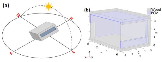
Figure 2.
Sketch of the studied issue; (a) location of the wooden house that is exposed to high outdoor temperatures and solar radiation; (b) geometry of the symmetric model used for computer simulations.
The present study will assess the influence of PCM panels covering the inner walls of a wooden house on the air temperature of its interior in the summer using output data obtained by computer simulations. The aim of the study is to create methods and tools for the fast and high-quality assessment of the thermal stability and thermal comfort of occupants in wooden houses in terms of preventing their overheating. The following sections describe how we formulated the tests of the models of wooden houses, including a physical background of the studied problem and the results obtained from the output data performed by simulations in a COMSOL user interface, which was subsequently processed and evaluated by MATLAB software (MathWorks Inc., Natick, MA, USA).
2. Methodology
In this section, we will describe how we formulated the models of the wooden house and we will outline the conditions that were used for computer simulation. COMSOL Multiphysics 5.3 software was used for computer simulations using the Finite element method. MATLAB 2020b was used for subsequent analysis and graphical processing of the output data from simulations. The aim of the simulations was to assess the effect of covering the walls inside a house with a layer of the PCM on its passive cooling during the high outdoor temperatures and solar radiation in summer.
2.1. Model Description
The 3D model of the wooden house was formulated in the Heat Transfer user interface of the COMSOL Multiphysics software, which includes tools for modeling of the non-stationary heat transfer by conduction, convection, and radiation, including surface-to-surface and solar radiation. Because the physical background of thermal processes of the studied problems is very complex, the formulated model is composed only of the basic elements that significantly influence the heat transfer between the house interior and outside environment, as shown in Figure 2.
In the present study, three variants of the model are compared with regard to the coverage of the walls with the PCM. Model is represented by a house in which the construction consists only of wooden walls without PCM coverage. In model , the wooden walls and ceiling of the house are covered by a thin layer of the PCM (see Figure 2b). In model , only a wall opposite the window (a back wall) is covered by the PCM. Given the limitations of computational time and the computer’s memory reduction, geometric symmetry was assumed, and the simulations were performed on one half of the house, as shown in Figure 2b.
2.2. Physical Background
The model was used to monitor the time evolution of the air temperature inside a wooden house that was exposed to time-varying conditions of the outdoor air temperature and solar radiation for seven summer days, as shown in Figure 3. From the physical point of view, this is a problem of non-stationary (i.e., time dependent) heat transfer during which both the temperature of the air inside the house and the temperature of all of the elements of its construction are functions of time t and spatial coordinates . The heat transfer between the outside environment and environment inside the house is caused by the temperature gradient due to the heat flows in the direction of decreasing temperature [46,47,48]. The formulated model includes both the transfer of thermal energy through the walls, ceiling, door, and window of the house and the transfer of heat by radiation due to solar radiation. The heat radiation and absorption of the wall surfaces inside the house are also considered.
The non-stationary heat transfer in a house covered by PCMs can be described by a governing Equation (1) [46,49]:
where T denotes the thermodynamic temperature, t denotes the time of the process, and v is the fluid velocity. is the thermal conductivity, is density, is the specific heat capacity. stands for the rate the inner heat-generation per unit volume.
Equation (1) includes the heat transfer by conduction in solid elements of the house, the heat convection in fluids (i.e., in the air inside the house), and the heat accumulation in the mass of a specific domain. The sum of this thermal energies is equal to the domain heat energy source. In the studied cases, neither a heat source nor active cooling was considered inside the house.
Next, we supposed the phase change of a PCM located inside the house. During this process, the PCM releases or absorbs a large amount of thermal energy. Therefore, the specific heat capacity of the PCM includes the latent heat and can be described by Equation (2) [49]:
where represents a material in a phase 1, represents material in a phase 2. denotes their volume fraction, and L is the latent heat.
A mass fraction of the solid and liquid phases can be expressed as follows:
For an assumption of a smooth transition over , with a phase mass fraction , it holds:
The effective thermal conductivity is defined as:
For the studied non-stationary heat transfer, the temperature and heat flow density on a surface were assumed, and a convective boundary condition can be described by Equation (6):
where the convective heat transfer depends on the heat transfer coefficient h, surface temperature , convective exchange temperature . is the incident radiant heat flow per unit surface area.
A condition describing the heat transfer by radiation was applied on boundaries between solid surfaces and the air. It can be expressed as follows:
Symbol denotes the surface emissivity, is the surface thermodynamical temperature, and is the thermodynamical ambient temperature. is Stephan-Boltzmann constant.
Finally, an external radiation source condition was used to simulate the influence of the solar radiation on the house, as depicted in Figure 2a. In the COMSOL Multiphysics user interface, the Sun’s radiation direction can be defined from the geographical position and time. A sunlight direction (zenith, angle, and the solar elevation) can be automatically calculated from the latitude, longitude, time zone in which the object is located, and the date and time of the simulated day.
2.3. Simulation Conditions
The supposed house was located in the Czech Republic region with geographic coordinates of the longitude 17.663 E, latitude 49.224 N, and altitude 250 m above sea level.
The structure of the walls of the house is shown in Figure 2b. Its internal length was 8 m. The width was 6 m, and the height was 3 m. Area of the window took of the front wall area. The PCM layer thick is 30 mm thickness, and it covers the selected walls and the ceiling inside the studied house.
The phase change temperature of the PCM was 22 C. The latent heat from solid and liquid phase , and the transition interval was 4 C. The thermal conductivity, density, specific thermal capacity, and emissivity of all geometrical elements used in the model are listed in Table 1. For simplification of the simulation, the temperature dependence of these parameters was neglected, and their mean values were used.
The initial temperature of the walls was 23 C. Initial temperature of the air inside the house was 24 C, and its velocity was . Figure 3a depicts the time evolution of the outside air temperature measured during 7 days in August. Figure 3b shows the solar radiation acting on walls of the studied house. The data were used from the Czech technical standard [50]. A floor was thermally insulated from the outside throughout simulations.

Figure 3.
Conditions of simulations; (a) the time evolution of temperature of the air outside the house and (b) solar radiation, from [51], based on solar radiation intensity recommendations [50].
Figure 3.
Conditions of simulations; (a) the time evolution of temperature of the air outside the house and (b) solar radiation, from [51], based on solar radiation intensity recommendations [50].


Table 1.
Properties of materials used in the tested models. From [51].
Table 1.
Properties of materials used in the tested models. From [51].
| Material | Thermal | Density | Specific | Emissivity |
|---|---|---|---|---|
| Conductivity | Heat Capacity | |||
| Wood | 0.18 | 400 | 2510 | 0.89 |
| Glass | 0.76 | 2600 | 840 | 0.96 |
| PCM | 0.18 0.14 | 800 | 9000 | 0.99 |
Thermal conductivity in solid phase. Thermal conductivity in liquid phase.
2.4. Simulation Settings
A free tetrahedral mesh was used to solve the studied problem. A mesh matrix density (degrees of freedom) was influenced on a geometric arrangement of the studied model. The size of the parameters of the model’s elements depended on their dimensions. The number of elements was between 123,258 (for the model with wood thickness of 0.4 m without a PCM) and 339,798 (for the model in which wood thickness was 0.4 m and PCM layers of thickness 30 mm covered all walls, except a floor). The quality of the mesh that we used was influenced by computer capability.
The simulation time took between 3 and 8 days, depending on the geometric arrangement of the studied model. The model was calculated on a computer with a processor Intel(R) Core(TM) i7-5820K CPU 3.30 GHz, with six cores. The available memory was 64 GB. The simulations were performed by the generalized minimal residual iterative method (GMRES). The maximum maximum allowed error of simulation steps was 0.1.
A time dependent study was applied for a time range from 0 h to 168 h. The time step was 2 h. The tested thickness of the wood walls was 0.2–0.4 m.
3. Results of the Simulations
The time evolution of the air temperature inside a tested wooden house for a time period of 7 days considering outdoor climatic conditions and geometric structure of the studied model is displayed in Figure 4. The values of the air temperature were evaluated in the middle of the house. In each of the studied models (i.e., , , ), the simulations were compared for the wood wall thickness of 0.2 m, 0.3 m, and 0.4 m. The results obtained for model of the house without the PCM coverage are depicted in Figure 4a. Temperature curves in model with walls, except a floor, covered by the PCM are shown in Figure 4b. Results for model in which only a back wall (i.e., a wall opposite the window) was covered by a PCM layer are depicted in Figure 4c. The results show considerable fluctuations in the daily air temperature in all of the houses as a reaction of changing the outdoor thermal conditions. However, a temperature increase during the tested time period is seen in all of the studied models. The maximum temperatures were 36.6 C for model , 34.7 C for model , and 32.8 C for model . In all of the studied cases, the dependence of temperature increase on the wood wall thickness was found. The maximum temperature difference with regards to wooden wall thickness was monitored in model , in which the maximum difference was 1.5 C.
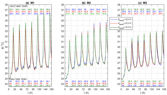
Figure 4.
The time evolution of the air temperature in the center of the house; (a) model : house without the PCM coverage; (b) model : house with all walls (except the floor) covered by the PCM; (c) model : house in which only the back wall is covered by the PCM. The wooden wall thickness is 0.2 m, 0.3 m, and 0.4 m.
A more detailed comparison of the effect of the PCM coverage on the temperature of the air inside the house is shown in Figure 5. Temperature differences were calculated for the air in the middle of the house in selected simulated times. Blue dots indicate differences between the air temperature in the house covered by PCM presented by model and model of the house without PCM coverage calculated according to relation . Red dots indicate differences between the air temperature in model with the PCM coverage and model without the PCM coverage calculated according to relation .
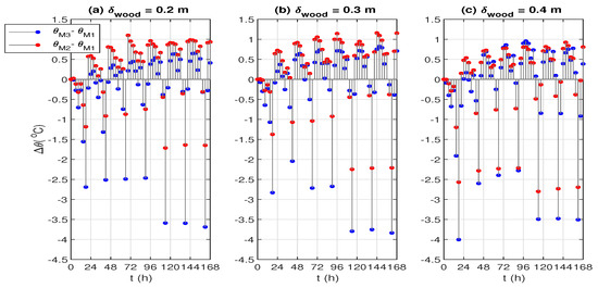
Figure 5.
Differences of the air temperature inside the house with the PCM coverage to the house without PCM coverage. Results for the house with wood wall thickness of (a) 0.2 m; (b) 0.3 m; (c) 0.4 m.
The results presented in Figure 5a were evaluated under the assumption that the thickness of the wooden wall is 0.2 m. In Figure 5b, the assumed thickness of the wooden wall is 0.3 m. In Figure 5c, the assumed thickness of the wooden wall is 0.4 m. The maximum temperature differences were found in the evening hours, when the house was most warmed due to actual climatic conditions. The air temperatures determined in the house with the PCM coverage in morning, afternoon and night hours were more in line with the air temperatures in a house without the PCM coverage. The maximum temperature difference was indicated for model with a wooden wall thickness of 0.2 m. In this case, at a simulated time of 162 h, the air temperature inside the house was 3.9 C lower than the temperature of the house without the PCM coverage.
Similarly, the maximum daily temperature differences between models and (except the first simulated day) were compared. If the thickness of the wooden wall was 0.4 m, then the daily maximum ranged from 2.2 C (at a simulated time of 90 h) to 2.8 C (at a simulated time of 114 h), as is shown in Figure 5c. For a wooden wall thickness of 0.3 m, the maximum daily differences between and were in the range of 0.9 C (at a simulated time of 90 h) to 2.2 C (at a simulated time of 114 h), as shown in Figure 5b. If the thickness of the wooden wall was 0.2 m, then the maximum daily differences between and were in the range of 0.7 C (at a simulated time of 90 h) to 1.7 C (at a simulated time of 114 h), as shown in Figure 5a.
By comparing the results of the simulations, the output data for the first simulated day were not evaluated. We supposed that they are not precise because we did not know some of the real initial conditions (e.g., the initial temperatures of the walls), so we only used estimated values for the simulations. Under this assumption, the temperature differences in daily maximum ranged from 2.3 C (at a simulated time of 90 h) to 3.5 C (at a simulated time of 162 h) by comparing models and with a wooden wall thickness of 0.4 m (see Figure 5c) for simulated days 2–7. The temperature differences between 2.0 C (at a simulated time of 42 h) and 3.9 C (at a simulated time of 162 h) were found for these models with a wooden wall thickness of 0.3 m (see Figure 5b). The differences approximately between 2.5 C (at a simulated time of 42 h) and 3.6 C (at a simulated time of 162 h) were found for models and with a wooden wall thickness of 0.2 m (see Figure 5a).
The simulations also allowed us to assess the thermal behavior of the walls and PCM located in the house. The thermal behavior of the PCM located in model is shown in Figure 6 and Figure 7. Figure 6 depicts a temperature distribution in a house with 0.3 m wooden walls thickness covered by the PCM in time 158 h when the maximum temperature of the air inside the house was achieved.
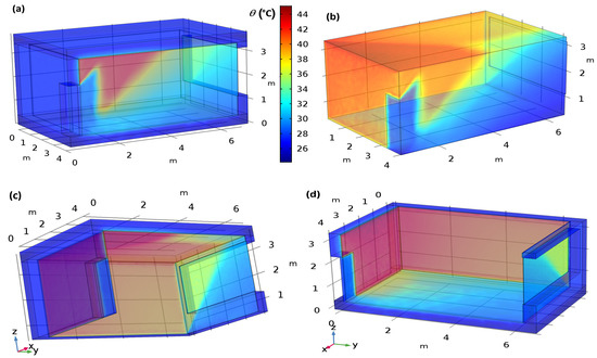
Figure 6.
Temperature distribution in model of 0.3 m wooden wall thickness covered by a PCM after 158 h; (a) completed model of the house; (b) air inside the house; (c) walls and a ceiling; (d) walls and a floor.
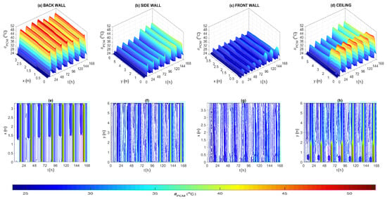
Figure 7.
Time evolutions of temperatures on PCM surfaces in model with the wood layer thickness of 0.3 m. (a,e) the 3D time evolution and 2D temperature field of the back wall (wall opposite the window). The temperature data are evaluated in the x direction from distance from a floor m; (b,f) the 3D time evolution and 2D temperature field of the side wall. The temperature data are evaluated in the height of 1.5 m in the y direction; (c,g) the 3D time evolution and 2D temperature field of the front wall (wall with a window). The temperature data are evaluated in height 0.4 m in the x direction; (d,h) the 3D time evolution and 2D temperature field of the ceiling. The temperature data are evaluated in distance m in the y direction.
Surface temperatures of the PCM layers covering all walls are shown in Figure 6c,d. It can be seen that surface temperatures of a floor and PCM layer applied on the front wall with the window are much lower than the surface temperatures of the PCM layer located on the side wall, back wall, and ceiling. The greatest accumulation of the thermal energy can be seen in the PCM covering the wall opposite the window. This is also reflected in the distribution of air temperature inside the house, as shown in Figure 6a,b.
The time evolutions of the temperature on the PCM surfaces are depicted in Figure 7. They show periodic changes of temperatures caused by changes in the intensity of sunlight passing through the window of the house and by changes in the temperature of the outside air.
Maximum and minimum PCM surface temperatures calculated in models and of 0.3 m wooden walls thickness for each simulated day are summarized in Table 2. They were calculated as average values of temperatures, which were determined in individual points of the mesh forming the given surface at a given time. By comparing the daily maximum temperatures, the highest value was achieved on the PCM surface of the back wall in model with all walls, except a floor, were coated by the PCM. In this case, the PCM surface temperature reached 50.9 C for the fourth simulated day. In model with a PCM-coated back wall, the maximum temperature of 49.5 C was determined, as seen in Table 2a.
Table 2.
Daily maximum and minimum temperature on the PCM surfaces.
The results listed in Table 2b show that the PCM surface temperatures did not reach higher values than 28.0 C at the times of daily minima. This value was calculated on the surface of the PCM located on the front wall of in the seventh simulated day. As was mentioned, the temperatures calculated for the first simulated day were not included in the evaluation. Under this assumption, the lowest temperatures in the daily minima were calculated on the surface of the PCM side wall, in which the temperature strongly depends not only on time but also on the distance from the window, as seen in Figure 7b,f.
4. Discussion
The optimum position to apply PCMs in building walls depends on many factors. For the optimal efficiency of PCMs, it is necessary to perform a daily complete melt-freeze cycle. The optimal PCMs’ application in building walls is influenced by many parameters, such as properties and quantity of PCMs, thermophysical properties of wall materials, indoor and outdoor thermal conditions, and the incident solar radiation [6].
The results of the computer simulations that have been presented in this study have confirmed that the incorporation of PCMs into the structure of a wooden house can affect the distribution and time evolution of the air temperature in its interior. The appropriate placement of PCMs on the inner walls of the house is essential for maintaining the required thermal comfort for the occupants, which proves a comparison of the time evolutions of indoor air temperature for the studied models and . In terms of passive cooling, model (in which only a back wall was covered by the PCM) was more efficient than model (in which all walls, except a floor, were covered by the PCM). This may be caused by the release of more thermal energy from the PCM material in model during the night.
For all of the studied models, the air temperature inside the house on each simulated day reached the highest values between approximately 4:00 p.m. and 6:00 p.m., which corresponds to time courses of the outdoor air temperature and solar radiation intensity with regard to the time delay of thermal transfer through the walls and windows of the house. The results obtained by comparing the efficiency of the PCM coverage in both of models and are summarized in Table 3. The values represent the percentage decrease in air temperature in models and with the PCM, relative to the air temperature of model without the CPM coverage. The values were compared at times when the air temperature inside the house reached a maximum for each simulated day. Data for the first simulated day were not included in the evaluation because these results were inaccurate due to the estimated initial conditions inserted into the models. The results proved the higher efficiency of the passive cooling in model (in which only a back wall was covered by the PCM) than in model (in which all walls, except a floor, were covered by the PCM). Under the studied conditions, the maximum efficiency reached 31.1% in the seventh simulated day.
Table 3.
Efficiency of the PCM coverage.
The results also showed that the PCM coverage can prevent an extreme increase in the air temperature in a house, especially in the afternoon and evening hours, when a house is most heated by the influence of outdoor conditions with respect to time lag between indoor and outdoor temperature courses [52,53]. However, the results of the simulations did not confirm that the coverage of the PCM walls would significantly affect the average daily temperature of the air inside the house under the considered conditions, as shown in Table 4a. This is probably related to the ability of PCMs to decrease air temperature fluctuations [32]. The average daily temperatures of the air inside the house were calculated as average values from temperatures in the middle of the studied house obtained by COMSOL Multiphysics for each time step of the simulation of the studied day.
Table 4.
Average daily temperature of the air inside the house and the range of temperature values.
The wooden wall thickness affects the thermal comfort of the indoor environment. In this study, the wood thickness was tested in the range of 0.2 m to 0.4 m because the walls of the studied model represent the outer walls of a wooden house. But, when assessing the effect of the interior walls of a building, it would be necessary to also analyze thicker walls.
The influence of the wood wall thickness in the range of 0.1 m to 0.5 m on the mean air temperature inside the studied model is depicted in Figure 8. The results showed that the maximum mean daily temperature difference was 0.8 C in the tested thickness range. Similarly, the maximum temperature differences were 0.6 C in daily minima of the indoor air temperature and 1.4 C in daily maxima of indoor air temperature.
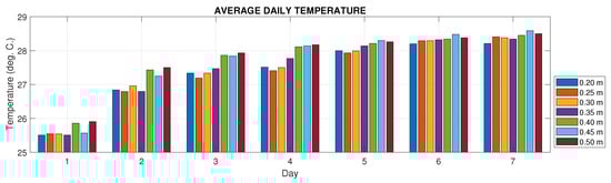
Figure 8.
Average daily temperature of the air inside the house with the wood wall thickness in the range of 0.2 m to 0.5 m.
5. Conclusions
Testing the influence of PCMs on the thermal stability and thermal comfort inside buildings by computer simulations has allowed us to obtain basic information for further detailed assessment of the studied issue, or for creating new architectural designs and proposals for changes in building renovations. The use of software tools for these purposes brings financial savings compared to real experiments and also gives us the ability to quickly obtain the desired results. The main parameters can be incorporated into formulated models of studied buildings, and the results can be compared by modifying these parameters.
On the other hand, there are a number of limitations that it is necessary to consider when performing computer simulations to test non-stationary thermal phenomena which are in many cases very complex. Therefore, computer simulations can be used as a support tool, but when compiling architectural designs in practice, it is necessary to supplement them with analysis under real conditions. In particular, these limitations include the need to simplify due to the limited memory of the computer that we used. Consequently, a spatially symmetric model was formulated in the present study. This enabled us to reduce the number of network points used for the calculation by half compared to the same model without using the symmetry condition. Next, the basic construction of the studied models was represented only by simple wooden walls.In addition, the PCM layer structure was very simple. Based on the results of a previous study [54], only a 30-mm thick PCM layer that is suitable for covering residential buildings was tested in the present study. To further simplify the calculation, average values of thermophysical properties of PCM for the studied temperature range were entered into the models instead of their the temperature-dependent values.
Furthermore, only thermal conditions were assessed in the present study, but there are many factors that influence indoor environment conditions. Therefore, it is expected that future work further research will include a more complex study of optimal indoor conditions for the health of individuals, including not only optimal thermal but also lighting factors in summer and winter for various kinds of residential buildings. In the present study, 7 summer days were assessed. But, it will be necessary to carry out a more detailed case study on a given day as a part of our research.
Author Contributions
Methodology, M.Z., H.C. and A.P.; Investigation, H.C.; Visualization, H.C. and A.P. All authors have read and agreed to the published version of the manuscript.
Funding
This work was supported by the European Regional Development Fund under the project CEBIA-Tech Instrumentation No. CZ.1.05/2.1.00/19.0376 and by the Ministry of Education, Youth and Sports of the Czech Republic within the National Sustainability Programme project No. LO1303 (MSMT-7778/2014).
Conflicts of Interest
The authors declare no conflict of interest.
Abbreviations
| Specific heat capacity, | |
| h | Heat transfer coefficient, |
| L | Latent heat, |
| n | Normal vector, |
| q | Heat flow density, |
| Incident radiant heat flow per unit surface area, | |
| t | Time, |
| T | Thermodynamic temperature, |
| Ambient temperature, | |
| External temperature, | |
| Surface temperature, | |
| Initial temperature of a body, | |
| v | Fluid velocity, |
| x, y, z | Space coordinates, |
| Vapor mass fraction, | |
| Wall thickness, | |
| Thermal conductivity, | |
| Inner heat-generation rate per unit volume, | |
| Density, | |
| Temperature, (C) | |
| Convective exchange temperature, (C) | |
| Surface temperature, (C) | |
| Volume fraction, | |
| Emissivity, | |
| Stephan-Boltzmann constant, | |
| Model of a wooden house without the PCM coverage | |
| Model of a wooden house with all walls, except a floor, covered by the PCM | |
| Model of a wooden house with back wall (i.e., wall opposite the window) covered by the PCM | |
| PCM | Phase change material |
References
- Czech Statistical Office Residential and Non-Residential Construction and Buildings Permits—Time Series. Available online: https://www.czso.cz/csu/czso/bvz_ts (accessed on 4 November 2020).
- Adekunle, T.; Nikolopoulou, M. Thermal comfort, summertime temperatures and overheating in prefabricated timber housing. Build. Environ. 2016, 103, 21–35. [Google Scholar] [CrossRef]
- CSN EN 16789-1, Energy Performance of Buildings—Ventilation for Buildings—Part 1: Indoor Environmental Input Parameters for Design and Assessment of Energy Performance of Buildings Addressing Indoor Air Quality, Thermal Environment, Lighting and Acoustics—Module M1-6; Office for Technical Standardization, Metrology and State Testing: Prague, Czech Republic, 2020.
- Saffari, M.; De Gracia, A.; Ushak, S.; Cabeza, L. Economic impact of integrating PCM as passive system in buildings using Fanger comfort model. Energy Build. 2016, 112, 159–172. [Google Scholar] [CrossRef]
- Bergia Boccardo, L.; Kazanci, O.; Quesada Allerhand, J.; Olesen, B. Economic comparison of TABS, PCM ceiling panels and all-air systems for cooling offices. Energy Build. 2019, 205. [Google Scholar] [CrossRef]
- Al-Absi, Z.A.; Isa, M.H.M.; Ismail, M. Phase change materials (PCMs) and their optimum position in building walls. Sustainability 2020, 12, 1294. [Google Scholar] [CrossRef]
- Barzin, R.; Chen, J.J.; Young, B.R.; Farid, M.M. Application of PCM underfloor heating in combination with PCM wallboards for space heating using price based control system. Appl. Energy 2015, 148, 39–48. [Google Scholar] [CrossRef]
- Yan, T.; Xu, X.; Gao, J.; Luo, Y.; Yu, J. Performance evaluation of a PCM-embedded wall integrated with a nocturnal sky radiator. Energy 2020, 210. [Google Scholar] [CrossRef]
- Li, Y.; Nord, N.; Xiao, Q.; Tereshchenko, T. Building heating applications with phase change material: A comprehensive review. J. Energy Storage 2020, 31. [Google Scholar] [CrossRef]
- Faraj, K.; Khaled, M.; Faraj, J.; Hachem, F.; Castelain, C. Phase change material thermal energy storage systems for cooling applications in buildings: A review. Renew. Sustain. Energy Rev. 2020, 119. [Google Scholar] [CrossRef]
- Qiao, Y.; Cao, T.; Muehlbauer, J.; Hwang, Y.; Radermacher, R. Experimental study of a personal cooling system integrated with phase change material. Appl. Therm. Eng. 2020, 170. [Google Scholar] [CrossRef]
- Tang, L.; Zhou, Y.; Zheng, S.; Zhang, G. Exergy-based optimisation of a phase change materials integrated hybrid renewable system for active cooling applications using supervised machine learning method. Sol. Energy 2020, 195, 514–526. [Google Scholar] [CrossRef]
- Zhou, Y.; Zheng, S.; Liu, Z.; Wen, T.; Ding, Z.; Yan, J.; Zhang, G. Passive and active phase change materials integrated building energy systems with advanced machine-learning based climate-adaptive designs, intelligent operations, uncertainty-based analysis and optimisations: A state-of-the-art review. Renew. Sustain. Energy Rev. 2020, 130. [Google Scholar] [CrossRef]
- Skovajsa, J.; Zalesak, M. The use of the photovoltaic system in combination with a thermal energy storage for heating and thermoelectric cooling. Appl. Sci. 2018, 8, 1750. [Google Scholar] [CrossRef]
- Li, G.; Bi, X.; Feng, G.; Chi, L.; Zheng, X.; Liu, X. Phase change material Chinese Kang: Design and experimental performance study. Renew. Energy 2020, 150, 821–830. [Google Scholar] [CrossRef]
- Gholamibozanjani, G.; Farid, M. A comparison between passive and active PCM systems applied to buildings. Renew. Energy 2020, 162, 112–123. [Google Scholar] [CrossRef]
- Rucevskis, S.; Akishin, P.; Korjakins, A. Parametric analysis and design optimisation of PCM thermal energy storage system for space cooling of buildings. Energy Build. 2020, 224. [Google Scholar] [CrossRef]
- Hussein, M. Improvements of building envelope using passive cooling techniques to reduce the cooling load in hot-dry regions. Heat Transf. Asian Res. 2019, 48, 3831–3842. [Google Scholar] [CrossRef]
- Web of Science Platform. Available online: https://apps.webofknowledge.com (accessed on 4 November 2020).
- Hawes, D.; Banu, D.; Feldman, D. Latent heat storage in concrete. II. Sol. Energy Mater. 1990, 21, 61–80. [Google Scholar] [CrossRef]
- Kolacek, M.; Charvatova, H.; Sehnalek, S. Experimental and numerical research of the thermal properties of a PCM window panel. Sustainability 2017, 9, 1222. [Google Scholar] [CrossRef]
- Pasupathy, A.; Velraj, R. Effect of double layer phase change material in building roof for year round thermal management. Energy Build. 2008, 40, 193–203. [Google Scholar] [CrossRef]
- Xu, X.; Zhang, Y.; Lin, K.; Di, H.; Yang, R. Modeling and simulation on the thermal performance of shape-stabilized phase change material floor used in passive solar buildings. Energy Build. 2005, 37, 1084–1091. [Google Scholar] [CrossRef]
- Scalat, S.; Banu, D.; Hawes, D.; Parish, J.; Haghighata, F.; Feldman, D. Full scale thermal testing of latent heat storage in wallboard. Sol. Energy Mater. Sol. Cells 1996, 44, 49–61. [Google Scholar] [CrossRef]
- Neeper, D. Thermal dynamics of wallboard with latent heat storage. Sol. Energy 2000, 68, 393–403. [Google Scholar] [CrossRef]
- Kuznik, F.; Virgone, J. Experimental investigation of wallboard containing phase change material: Data for validation of numerical modeling. Energy Build. 2009, 41, 561–570. [Google Scholar] [CrossRef]
- Lai, C.-M.; Chen, R.; Lin, C.Y. Heat transfer and thermal storage behaviour of gypsum boards incorporating micro-encapsulated PCM. Energy Build. 2010, 42, 1259–1266. [Google Scholar] [CrossRef]
- Hasse, C.; Grenet, M.; Bontemps, A.; Dendievel, R.; Sallée, H. Realization, test and modelling of honeycomb wallboards containing a Phase Change Material. Energy Build. 2011, 43, 232–238. [Google Scholar] [CrossRef]
- Kuznik, F.; Virgone, J.; Johannes, K. In-situ study of thermal comfort enhancement in a renovated building equipped with phase change material wallboard. Renew. Energy 2011, 36, 1458–1462. [Google Scholar] [CrossRef]
- Zhou, D.; Zhao, C.; Tian, Y. Review on thermal energy storage with phase change materials (PCMs) in building applications. Appl. Energy 2012, 92, 593–605. [Google Scholar] [CrossRef]
- Baetens, R.; Jelle, B.P.; Gustavsen, A. Phase change materials for building applications: A state-of-the-art review. Energy Build. 2010, 42, 1361–1368. [Google Scholar] [CrossRef]
- Kuznik, F.; Virgone, J.; Noel, J. Optimization of a phase change material wallboard for building use. Appl. Therm. Eng. 2008, 28, 1291–1298, cited By 180. [Google Scholar] [CrossRef]
- Soares, N.; Costa, J.; Gaspar, A.; Santos, P. Review of passive PCM latent heat thermal energy storage systems towards buildings’ energy efficiency. Energy Build. 2013, 59, 82–103. [Google Scholar] [CrossRef]
- Sun, W.; Zhang, Y.; Ling, Z.; Fang, X.; Zhang, Z. Experimental investigation on the thermal performance of double-layer PCM radiant floor system containing two types of inorganic composite PCMs. Energy Build. 2020, 211. [Google Scholar] [CrossRef]
- Kong, X.; Wang, L.; Li, H.; Yuan, G.; Yao, C. Experimental study on a novel hybrid system of active composite PCM wall and solar thermal system for clean heating supply in winter. Sol. Energy 2020, 195, 259–270. [Google Scholar] [CrossRef]
- Wang, T.; Guan, Y.; Hu, W.; Yang, H.; Guo, J.; Zhang, R. Experimental study on improving thermal environment in solar greenhouse with active—Passive phase change thermal storage wall. Environ. Sci. Eng. 2020, 1243–1252. [Google Scholar] [CrossRef]
- Hagenau, M.; Jradi, M. Dynamic modeling and performance evaluation of building envelope enhanced with phase change material under Danish conditions. J. Energy Storage 2020, 30. [Google Scholar] [CrossRef]
- Ye, R.; Huang, R.; Fang, X.; Zhang, Z. Simulative optimization on energy saving performance of phase change panels with different phase transition temperatures. Sustain. Cities Soc. 2020, 52. [Google Scholar] [CrossRef]
- Zhu, N.; Li, S.; Hu, P.; Lei, F.; Deng, R. Numerical investigations on performance of phase change material Trombe wall in building. Energy 2019, 187. [Google Scholar] [CrossRef]
- Guan, Y.; Wang, T.; Tang, R.; Hu, W.; Guo, J.; Yang, H.; Zhang, Y.; Duan, S. Numerical study on the heat release capacity of the active-passive phase change wall affected by ventilation velocity. Renew. Energy 2020, 150, 1047–1056. [Google Scholar] [CrossRef]
- Li, M.; Gui, G.; Lin, Z.; Jiang, L.; Pan, H.; Wang, X. Numerical thermal characterization and performance metrics of building envelopes containing phase change materials for energy-efficient buildings. Sustainability 2018, 10, 2657. [Google Scholar] [CrossRef]
- Herbinger, F.; Desgrosseilliers, L.; Groulx, D. Thermal Modeling in a Historical Building—Improving Thermal Comfort through the Siting of a Passive Mass of Phase Change Material; COMSOL Inc.: Boston, MA, USA, 2014; pp. 1–7. [Google Scholar]
- Kylili, A.; Theodoridou, M.; Ioannou, I.; Fokaides, P. Numerical Heat Transfer Analysis of Phase Change Material (PCM)—Enhanced Plasters; COMSOL Inc.: Munich, Germany, 2016; pp. 1–7. [Google Scholar]
- Gerlich, V.; Sulovska, K.; Zalesak, M. COMSOL Multiphysics validation as simulation software for heat transfer calculation in buildings: Building simulation software validation. Measurement 2013, 46, 2003–2012. [Google Scholar] [CrossRef]
- Neymark, J.; Judkoff, R. International Energy Agency Building Energy Simulation TEST and Diagnostic Method (IEA BESTEST). In-Depth Diagnostic Cases for Ground Coupled Heat Transfer Related to Slab-on-Grade Construction; National Renewable Energy Laboratory: Golden, CO, USA, 2008; pp. 549–572.
- Carslaw, H.; Jaeger, J. Conduction of Heat in Solids; Clarendon Press: Oxford, UK, 1992. [Google Scholar]
- Fan, Y.; Xu, K.; Wu, H.; Zheng, Y.; Tao, B. Spatiotemporal modeling for nonlinear distributed thermal processes based on KL decomposition, MLP and LSTM network. IEEE Access 2020, 8, 25111–25121. [Google Scholar] [CrossRef]
- Khovanskyi, S.; Pavlenko, I.; Pitel, J.; Mizakova, J.; Ochowiak, M.; Grechka, I. Solving the coupled aerodynamic and thermal problem for modeling the air distribution devices with perforated plates. Energies 2019, 12, 3488. [Google Scholar] [CrossRef]
- COMSOL. Heat Transfer Module User’s Guide; v. 5.3 Edition; COMSOL Multiphysics: Stockholm, Sweden, 2017. [Google Scholar]
- CSN 73 0540-3, Thermal Protection of Buildings—Part 3: Design Value Quantities; Office for Technical Standardization, Metrology and State Testing: Prague, Czech Republic, 2005. (In Czech)
- Charvatova, H.; Zalesak, M.; Kolacek, M.; Sehnalek, S. Experimental and Numerical Testing of Possibilities and Limits for Applications of Phase Changed Materials in Buildings. MATEC Web Conf. 2019, 292. [Google Scholar] [CrossRef]
- Oktay, H.; Yumrutas, R.; Argunhan, Z. An experimental investigation of the effect of thermophysical properties on time lag and decrement factor for building elements. Gazi Univ. J. Sci. 2020, 33, 492–508. [Google Scholar] [CrossRef]
- Jannat, N.; Hussien, A.; Abdullah, B.; Cotgrave, A. A comparative simulation study of the thermal performances of the building envelope wall materials in the tropics. Sustainability 2020, 12, 4892. [Google Scholar] [CrossRef]
- Charvatova, H.; Prochazka, A.; Zalesak, M. Computer simulation of temperature distribution during cooling of the thermally insulated room. Energies 2018, 11, 3205. [Google Scholar] [CrossRef]


Publisher’s Note: MDPI stays neutral with regard to jurisdictional claims in published maps and institutional affiliations. |
© 2020 by the authors. Licensee MDPI, Basel, Switzerland. This article is an open access article distributed under the terms and conditions of the Creative Commons Attribution (CC BY) license (http://creativecommons.org/licenses/by/4.0/).