Abstract
This paper presents a controller design process for an aircraft tracking problem when not all states are available. In the study, a nonlinear-transport aircraft simulation model was used and identified through Maximum Likelihood Principle and Extended Kalman Filter. The obtained mathematical model was used to design a Linear–Quadratic Regulator (LQR) with optimal weighting matrices when not all states are measured. The nonlinear aircraft simulation model with LQR controller tracking abilities were analyzed for multiple experiments with various noise levels. It was shown that the designed controller is robust and allows for accurate trajectory tracking. It was found that, in ideal atmospheric conditions, the tracking errors are small, even for unmeasured variables. In wind presence, the tracking errors were proportional to the wind velocity and acceptable for small and moderate disturbances. When turbulence was present in the experiment, state variable oscillations occurred that were proportional to the turbulence intensity and acceptable for small and moderate disturbances.
1. Introduction
The growth of commercial aviation results in increased requirements for the guidance systems as they need to provide better capabilities of the system while not lowering the safety level. Disturbances that act on the object (e.g., wind) can cause departure from the planned trajectory and thus lead to potentially dangerous situations. Moreover, if aircraft follows the prescribed path accurately, it is possible to optimize certain flight segments in order to save time and cost e.g., by using continuous descent operations [1]. Thus, the aircraft trajectory tracking problem is of great interest [2,3,4,5,6,7].
The full-state Linear–Quadratic Regulator (LQR) controller was successfully applied for trajectory tracking for various aircraft: fixed-wing [6,8,9], helicopters [10,11] and UAVs [12,13]. In case of incomplete state information, the LQG controller can be used instead. In [14] the LQG controller was designed to handle the tracking task for a linear business jet aircraft. In [15] a controller was designed for a nonlinear system that was sequentially linearized for missile path-following. In [16] the system stability is regained by using a LQG controller. A different approach is used in [17] to handle with the partial information- reduced-order observer is used to estimate unmeasured states.
The tracking problem can be also solved by using model predictive control (MPC). In this approach an object representation is used to predict the dynamic response of the object and basing on this information optimal control strategy is found. In [18] a nonlinear MPC was used to deal with tracking of a small-scale helicopter with unmodelled dynamics for a box manoeuvre in turbulent conditions. In [19] a nonlinear MPC was used to track fixed wing UAV in extreme manoeuvres (fast turn, sharp turn, flip), in case of actuators failures and for obstacle avoidance. The MPC was also used for off-road unmanned ground vehicle path tracking with taking into account sliding and steering constrains [20].
In the paper we propose another, new approach—to use LQR in which unmeasured states were directly omitted.
More precisely, this is a LQR problem with static output feedback, where the gain matrix is derived from the optimal gain matrix of the standard LQR problem by simply deleting columns corresponding to these state vector coordinates which are not present in the output vector. This simple construction proved to be very effective. We show conditions when it can be applied, that is, when the resulting closed-loop system is asymptotically stable. This approach requires an accurate model representing the aircraft dynamics, however, that can be obtained using system identification techniques. Several methods can be used for that purpose and those related to aerodynamic modelling are presented, e.g., in [21]. The most popular approach is the output-error method, which was used in numerous applications including icing modelling [22], missile microspoiler parameters estimation [23], aerodynamic coefficients identification [6,24] and performing near real time data compatibility check [25]. However, the output-error approach does not allow for process noise presence and thus aerodynamic turbulence strongly affects the identification quality. The problem is solved by including Kalman filter. In [26] the stability and control derivatives of the linear model were found by using this approach. In [27] the linear Kalman filter was used around the trim points to find the nonlinear model. A more common approach when dealing with nonlinear aircraft models is to use the Extended Kalman Filter. In [28] this was done for kite flight path reconstruction. Aerodynamic coefficients were estimated by using this approach in [29]. The nonlinear model can be also considered when Unscented Kalman Filter is introduced as in [30] for dealing with upset flight conditions. Unscented Kalman filter was also applied to identify a fixed-wing aircraft and a rotorcraft in [31]. Those results were compared with Extended Kalman Filter outcomes and time domain output error approach. It was found that the computational load of the Unscented Kalman Filter is at least twice of the Extended Kalman Filter and it does not result in significant gain in convergence or accuracy when aerodynamic coefficients are estimated [32]. Another possibility to deal with environmental uncertainties was presented in [33] where a nonlinear observer supplied by a Kalman Bucy filter was used to adjust tire–ground parameters in near-real time.
This paper is organized as follows. A nonlinear aircraft simulation model is presented in Section 2. In the remaining part of the paper this model is a treated like a real aircraft. This approach is often used in flight dynamics, as it allows to reduce costs when new designs or system modifications are tested [34,35]. In Section 3 the algorithm used for identifying the aircraft aerodynamic coefficients is shown. Estimation results and their validation is presented in this part as well. Problem formulation (trajectory tracking) is shown in Section 4. To solve this task a LQR controller was designed thought the approach shown in Section 5. The case scenario is presented in Section 6. The final outcomes are shown in Section 7. This is done for ideal atmospheric conditions and under atmospheric disturbances (wind, turbulence). The paper ends with short conclusions summary.
The novelty is twofold. First, the system identification approach with Kalman filtering is used to obtain an accurate nonlinear aircraft model for LQR design to track the aircraft trajectory. The second aspect of the novelty is related to the state measurements unavailability. In the case of incomplete state measurements a common practice is to use a LQG controller. In this paper we show that it is possible to solve our problem also by LQR with static output feedback—that is, without the restoration of the full state vector by an observer or a filter—applying gain matrices calculated during standard LQR controller synthesis. We explain when this method can be applied (in Section 5).
2. Nonlinear Aircraft Model
In the study, the Basic Aircraft Model (BACM) was used to represent the real aircraft. This is a nonlinear aircraft simulation model developed in the Matlab/Simulink environment. Besides aircraft dynamics, BACM also contains environment and sensors models. The environment model is based on International Standard Atmosphere model and WGS-84 system. Throttle position, aileron, elevator and rudder deflections are the inputs for the model. Model outputs consist of aircraft position and attitude, linear velocity components and angular rates, linear acceleration components and aerodynamic angles. Those elements are obtained from a IMU model (consisting of three-axis accelerometer and three-axis rate gyro) and pressure tube model.
The reason for BACM selection was twofold. First, using simulation models in flight dynamics is a common practice as it allows us to greatly lower the costs when new modifications or updated algorithms are to be assessed. Secondly, this would allow for direct comparison with [6] where BACM model was used for trajectory tracking when all states measurements were available.
The BACM is a nonlinear simulation model described in body axes. Equations of motion are obtained from momentum and angular momentum change theorems [36]:
where F and are external force and moment, is the angular rate and the dot symbol denotes time derivative.
The object is treated as rigid body, which centre of gravity coincides with the origin of the body axes frame (). The coordinate frame is shown in Figure 1.
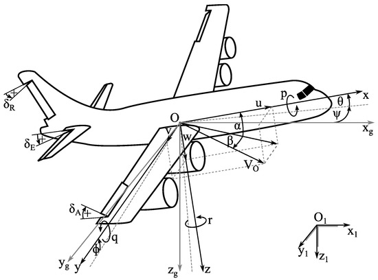
Figure 1.
Body axes system, state and control variables.
As the system identification experiment lasts for a short period of time, fuel consumption is neglected i.e., mass is assumed constant. Moreover, the airplane has a vertical symmetry plane in terms of geometry and mass. Due to those assumptions momentum and angular momentum are given as [36]:
where is the linear velocity, m stands for mass and I is the inertia matrix in which and .
This leads to the following equation set [36]:
where u, v and w are linear velocity components, p, q and r are angular velocity components, and are roll and bank angles, is the dynamic pressure, S is the wing area and and b stand for mean aerodynamic chord and wingspan, respectively.
The aerodynamic coefficients are given as [37]:
where and are angle of attack and sideslip angle, , and and ailerons, elevator and rudder deflections, k is the drag polar coefficient, is the horizontal tail arm denotes wing-body and H index stands for horizontal tail. The aerodynamic angles were obtained directly from linear velocity components: and . In the aerodynamic coefficients expressions, , , stand for lift, side and drag force aerodynamic biases and , , are rolling, pitching and yawing aerodynamic moment biases. The nondimensional coefficients express the i-th force or moment coefficient change due to j-th flight parameter or control, e.g., is the rolling moment coefficient change due to sideslip angle. The cross-coupling derivatives represent the i-th force or moment coefficient change due to k-th flight parameter effect on j, e.g., is the yawing moment coefficient change due to yaw rate resulting from angle of attack change.
The model was excited with D-optimal multi-step inputs presented in [37]. In that study, it was shown that designed inputs can provide accurate results for this aircraft if the flight is performed in calm atmosphere. The inputs are shown in Figure 2.
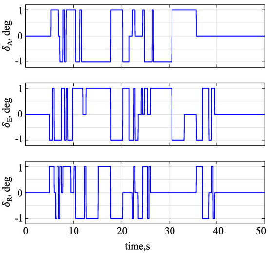
Figure 2.
Input signals.
While the model response was evaluated the states (u, , , p, q, r, , ) were corrupted by the process noise inclusion. After the evaluations, measurement noise was added to the outputs (states and acceleration components, i.e., , and ). From this point, the nondimensional aerodynamic parameters were considered as unknowns that must be estimated.
3. Aircraft System Identification
Presented aircraft model can be described by the following equations [32]:
where f and g are nonlinear functions, x, y and z are states, outputs and measurements, respectively, u is control, are model parameters, w and are process and measurement noise, whilst F and G are their distributions and is time at discrete k-th point.
The unknown parameters can be found by using the maximum likelihood principle. In this approach, a set of parameters that maximize conditional probability of observing measurements z is found [32]:
For the multidimensional normal distribution, the probability density function is given as:
The same result is obtained by performing a simpler task—minimization of the negative log-likelihood [32,37]:
where tilde symbol denotes predicted value. To estimate the residuals covariance matrix following formula can be used [32,37]:
For uncorrelated measurements errors and after neglecting constant terms the cost function simplifies to [32,37]:
In the study, the aircraft response was recorded in turbulent conditions. Due to process noise presence (turbulence), it was not possible to use the output error method, which is the most frequently used system identification method. To solve this issue, a Kalman filter was incorporated in the estimation algorithm accordingly to [32]. Resulting filter error method, which can be seen as the output error method extension, allows also for less local minima and faster convergence. To achieve this aim, the unknown parameters vector consists of model parameters and process noise distribution .
On the other hand, one has to bear in mind that the filter error method will allow us to obtain good match between the identified outputs and measurements even if the estimates are inaccurate. Thus, when performing the identification, special attention must be paid to statistical properties of the estimates. Moreover, using data from multiple experiments (for which process noise is different) requires estimating multiple process noise distributions.
Nonlinear model is incorporated into the Kalman filter prediction step to estimate the state variables x and outputs y [32]:
The correction step is given as [32]:
The steady-state Kalman gain matrix is used, as the nonlinearities are not large and the system is time invariant [32]:
The output matrix is found through numerical linearization:
State prediction error covariance matrix P is obtained by solving the Riccati equation [32]:
The equation can be solved by eigenvector decomposition (Potter’s method). First, the Hamiltonian matrix is build [32]:
After evaluating its eigenvectors and eigenvalues, those eigenvectors are sorted in descending order with respect to real parts of their corresponding eigenvalues. The obtained eigenvectors rearranged matrix is further decomposed [32]:
Finally, the state prediction error covariance matrix P is given as [32]:
To perform cost function minimization Gauss-Newton algorithm was used to estimate the aerodynamic coefficients [32]:
where the Fisher Information matrix is given as [32]:
and the gradient matrix is as follows [32]:
Finite difference approximation is used to evaluate gradients of each model response j for each model parameter l:
where is the l-th parameter small perturbation and e is a column vector with 1 in l-th row and zeros elsewhere. Evaluation of the predicted outputs when the model parameters are perturbed requires evaluation of the predicted states and corrected states for the perturbed parameters as well. This is done by evaluating (11) and (13) for the perturbed parameters .
To provide that the measurement noise covariance matrix is physically meaningful it must be positive-semi definitive. This is true when all eigenvalues of are real and less than one. The matrix tends to be diagonal-dominant, thus, the condition can be approximated by verifying if the diagonal elements satisfy the condition. The nonlinear inequality constraints can be approximated by [32]:
If this is satisfied for all conditions, the iteration is complete. Otherwise, the solution is given by [32]:
The gradient in constrained equation M is [32]:
where and are element indices, is the violated constrains number and is the estimated parameters number.
The auxiliary vector is [32]:
In the method, the R is estimated when all other parameters are fixed, and their values are estimated for fixed R. This approach works well if there is no strong correlation between those two. When the strong correlation exists the matrix is updated to compensate for revised R. This is done by using a heuristic procedure [32]:
where , , are indices, is the number of process noise variables being estimated, while old and new denote former and updated terms.
The described filter error method was used to identify nondimensional aerodynamic derivatives. We used the BACM model without assuming any knowledge of the aerodynamic derivatives, as in a case of dealing with true aircraft. To determine the aerodynamic coefficients, we identified the system by using the described Filter Error Method. When performing the system identification, we assumed initial values of the aerodynamic derivatives based on general flight dynamics knowledge (e.g., phugoid motion due to potential and kinetic energy conversion), empirical formulas [38] and aerodynamic derivatives values for similar aircraft. As estimating to many parameters at the same time may lead to local minima (and thus less accurate results), extends the estimation time and lowers convergence, a two-stage procedure was adopted. This approach was possible because cross-coupling had a secondary effect on aircraft dynamics.
Step 1a: first, while performing the identification it was assumed that u, , q and have primary influence on longitudinal motion. Those components formed the state vector used to evaluate the outputs. Besides mentioned state variables, the output vector consisted of longitudinal and vertical acceleration ( and ) for better convergence. The remaining motion variables (, p, r, , ) were weighted by 0, thus lateral-dimensional dynamics did not influence the longitudinal motion outcomes. In this step only the coefficients related to longitudinal motion were identified (, , , , , , ). The remaining aerodynamic derivatives were kept fixed at their initial values.
Step 1b: then, it was assumed that , p, r and influence mainly the lateral-directional motion. Besides mentioned state variables, the output vector consisted of lateral acceleration for better convergence. The remaining motion variables (u, , q, , and ) were weighted by 0, thus longitudinal dynamics did not influence the lateral-directional motion outcomes. In this step only the coefficients related to lateral directional motion were estimated (, , , , , , , , , , , , , , , , , ). The remaining aerodynamic derivatives were kept fixed at their previous values (i.e., estimated from longitudinal motion data in Step 1a).
Step 2: in the second stage, all state variables and acceleration components formed the output vector. The cross-coupling derivatives (, , , , , ) were also included in the estimation, i.e., all aerodynamic derivatives were identified. The values of the aerodynamic derivatives in the first iteration were taken from the estimates obtained when only longitudinal and only lateral-directional data was used (Step 1a and Step 1b, respectively).
In each step (Steps 1a, 1b, 2) the estimation was stopped when the relative change of the cost function in (10) was smaller than 1 × 10.
Relative deviations of the estimated aerodynamic coefficients are shown in Table 1. A rule of thumb is that relative standard deviations below 10% denote accurate estimates [32]. From the obtained outcomes, it can be seen that all the parameters were estimated with high precision. The results are also comparable with the outcomes obtained in previous studies [6]—when process noise was not present in the data and thus output error method was used.

Table 1.
Relative standard deviations, %.
The estimated model was also validated by feeding it with the data not used during system identification and comparing obtained time histories with the measured ones. This is shown in Figure 3, where blue lines denote measured responses and red lines stand for the estimated model outputs.
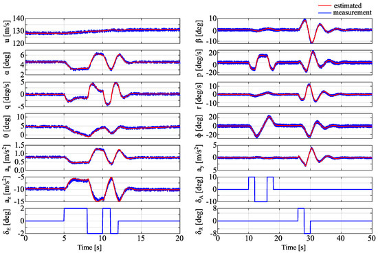
Figure 3.
Model verification.
From Figure 3 it can be seen that a very good visual match was obtained for the estimated model. To express this match quantitatively was used [39]:
where W is a diagonal weighting factor matrix. When the observations are in given in ft/s, ft/s, rad or rad/s the denotes high accuracy of the estimates if a six-DoF model with cross-coupling effects is used [39]. In the study, longitudinal velocity u and linear acceleration components , , were given in m/s or m/s, respectively. Therefore, a factor of 0.3048 was selected for those outputs in the weighting matrix W. The remaining non-zero elements in the weighting matrix were set to 1. In result the , what indicates high accuracy of the estimates and supports previous outcomes. To assess the estimated model predicting capabilities Theil Inequality Coefficient can be used [39]:
A rule of thumb is that indicates good predicting capabilities [39]. The obtained for the validation data was . Thus, it also confirms that the model was estimated with high precision.
4. Output Tracking Problem in Aircraft Modelling
Aircraft model development and verification leads to the output tracking problem, inherently. Availability of the aircraft state vector is crucial for it. However, the aircraft full state vector usually is not measured: side velocity, angular rates or WGS Cartesian coordinates are not used in standard flight control. Environmental state is known only partially: GPS can be used to obtain wind velocity and direction, but vertical air velocity is usually unknown. Usually, Pitot tube is used to measure angle of attack and sideslip angle, but it is also possible to obtain aerodynamic angles from measured velocity components or by using five-hole differential pressure probe. Another approach is to use Flush Air Data System, but this system needs to be designed, especially for each particular aircraft type. In practice, turbulence parameters are not available and can be identified for, e.g., Dryden or von Karman spectra. Air density , crucial in flight mechanics applications is hard to measure and can be obtained only indirectly from ideal gas law.
Thus, the tracking problem in aviation is then essentially an output tracking problems in which number of measurements m is usually less than state dimension n, .
The output tracking problem can be formulated in general as follows:
Given the measurements and inputs of a real aircraft and registered atmospheric conditions, find the inputs that provide the computed aircraft model outputs to be close to the measurements. Optionally, controls providing the outputs and the measurements matching should be close to those recorded in flight.
The success in tracking problem handling essentially depends on data availability and accuracy. If all states of an aircraft are available, the computed control should assure the state local error minimization with regard to the recorded state . In output tracking problem one should require control u that uniformly minimizes local error of the output with regard to the measurements .
In case of incomplete state measurements, when , much less accuracy of tracking error is to be expected, in general. The control that realizes output tracking is expected to be less regular than that obtained in tracking based on full state measurement. Issues that concern controlability and stabilizability will hardly influence control evaluation for output tracking problem.
The tracking problem is of an evolution type that makes use of recorded data given in long sampled time series. Thus, the time-domain approach are in favour over the frequency domain methods for its analysis.
There are several possibilities of handling the output tracking problems in time domain. The simplest one, based on classical PID controllers, is rather precluded because of large dimension of problem (greater than twelve) and strong cross dependencies between the system states.
The robust H-type (, , ) method defined in the frequency domain (e.g., [40,41]) can be formulated in time domain, but this require selection of pre- and post-compensator modules for plant (aircraft) dynamics, which is very difficult for real systems.
The most common approach to the output tracking problem is to use the Linear Quadratic Gauss regulator (LQG). It makes use of Kalman filter to restore the state vector from measurements in some stochastic sense. It is widely known that LQG was very successful in a variety of aerospace applications [40]. However, the LQG control requires knowledge (or assumption) on probabilistic characteristics of model and measurements disturbances, which are assumed to be Gaussian. Such information is rarely known in practice, that makes the use of LQG problematic in the considered output tracking problem.
In the present work, the LQR with static output feedback is proposed for handling the output tracking problem. This version of LQR is not widely used, but it will be shown here that the LQR can be applied successfully if some conditions (concerning detectability and stabilizability of the system, but not only) are fulfilled [42,43]. It will be shown that the robustness of LQR seems to be enough for assuring good properties of the controller in output tracking problem considered here.
5. LQR with Static Output Feedback
The output tracking problem can be solved by a LQR optimal control. The LQR working principle with incomplete states observation is presented in Figure 4.
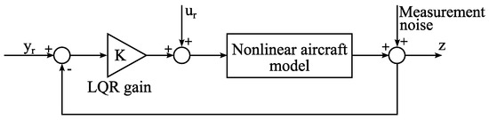
Figure 4.
LQR working principle.
The LQR control problem consists in the determination of the output feedback control law (index o indicates the output feedback) [40,42]
where and are output and control vectors at time t, and m, p are dimensions of control and output, respectively. The controller design process applied in the study is shown in Figure 5.
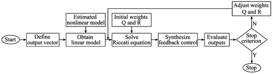
Figure 5.
Linear–Quadratic Regulator (LQR) design flowchart.
The optimal control law of type (32) is found by solving the constrained optimization problem where is a quadratic performance index which will be minimized
with the initial state , where n is the dimension of the state space and weighting matrices and for state and control, respectively. The constrains are given by the control law (32), together with the linear plant and output models
with initial conditions
where , and are the state, control and output matrices, respectively. It is assumed that the initial state is a random variable of a known probability distribution.
If the full state is measured, , the initial state is given as a (deterministic) vector of numbers and we have the classical LQR problem:
Index s of the control law indicates the state feedback.
When [44]:
- Q matrix is positive semidefinite,
- matrix R is strictly positive definite,
- the pair is stabilizable, and the pair , where D is such that is detectable,
the solution of the LQR problem (37)–(40) exists and is given by a stationary, linear control law
in which the optimal gain matrix is calculated as
where is the unique, positive semidefinite, symmetric solution of the stationary Riccati equation
Moreover, the closed-loop dynamic system (38) and (40), now with the dynamics
is asymptotically stable and the criterion (37) takes the value:
LQR control has favorable robustness properties, e.g., in SISO case: infinite gain and 60 phase margin and thus is appealing in various applications.
Unfortunately, it is not the case when output is given by (35) and . However, as we will show, the gain matrix , that is the solution of the standard LQR problem, can still be used.
In [45] it is assumed, that control is generated also via output linear feedback with time-invariant feedback gains, i.e., in (32):
and the optimization problem (33)–(36) can be rewritten as:
In the case, when the state transformation matrix
is stable, that is its eigenvalues lie in the negative halfplane, and, as in [45], the initial state is a random variable uniformly distributed on the surface of the n-dimensional unit sphere, in order for to be optimal it is necessary that , positive semidefinite and positive definite are solutions of the system of nonlinear equations [42,45]:
where is given by (51). The optimal value of the criterion (48) is:
Unfortunately, unlike the standard LQR problem with state feedback (37)–(40), Equations (52)–(54) are only necessary conditions, and there might be several solutions of these equations which are not optimal [45]. Moreover, conditions for the existence and global uniqueness of solutions to (52)–(54) such, that is positive semidefinite, is positive definite and the matrix
is stable are not known [46]. The latter problem itself is often cited as one of the difficult open problems in systems and control for which a satisfactory answer has yet to be found [43,47,48].
The algorithms solving LQR problem with output feedback were proposed by many authors [42]. The most popular solve many times the Riccati Equations (52) and (53) for properly changed, fixed matrices [42,45,49]. A basic issue for all of them is the selection of an initial stabilizing static output feedback gain [42]. Methods proposed in [42] are quite complicated. Since it is a very difficult problem, perhaps NP-hard [47], heuristic methods can be proposed, which proved to be effective while solving specific problems.
One of the specific class of problems is when the output vector y is formed by some of the coordinates of the state vector x. Let us denote the set of indices of x present in y as Z (it may be ordered, but it is not necessary). Hence, we may write:
The matrix C will be then formed from the n-dimensional row versors corresponding to subsequent elements of the set Z, that is
Let us take as a stabilizing gain matrix the submatrix of the matrix , being the optimal solution of the standard (that is with state feedback) LQR problem (37)–(40), which contains only columns corresponding to the coordinates of the vector y, that is
The closed-loop system (49) will take the form:
Let us notice that the matrix
is built of versors and n-dimensional vectors of zeros. A versor is in the i-th column of W when , that is the coordinate of the state vector is one of the coordinates of the output vector y. The remaining columns contain zeros. We may write:
where is the characteristic function of the set Z:
Let us denote by the -th row of the matrix B, by the j-th column of the matrix and by H the product of matrices B and . We will have:
Let us now apply the Gershgorin circle theorem [50] to the solution of the standard LQR problem (37)–(40). The LQR theory guarantees, that the system with matrix is asymptotically stable. Assume that the sufficient condition resulting from the Gershgorin theorem is satisfied, that is for all rows of there is:
and
Our system matrix in the case of the output feedback is
The matrix is simply the matrix H with zeroed columns corresponding to those coordinates of the state vector x, which were not taken to the output vector y, that is having indices . Hence, the Gershgorin conditions for all the eigenvalues of the matrix to have negative real parts will take the form:
Comparing (69) with (66) we obtain that when the matrices A and H satisfy the conditions:
that is, when the matrices A, B and , making use of (64), satisfy the conditions:
and from (66) and (68)
the closed-loop system with linear output feedback (60) for is asymptotically stable. It is not a solution of the problem (48)–(50) itself, but of a different LQR problem with output feedback, where some matrices were modified [43].
In LQR problems there are no constraints either on the current control , nor on the current state . Such problems, including those with mixed functional constraints on current control and state are very important in many areas of engineering. The methods of their solutions are presented e.g., in [51,52].
6. Case Scenario
The task is to compute the control for a cargo aircraft resulting in its flight path close to a given trajectory with time synchronization. In other words, aircraft should track the trajectory at the same time time points as during the flight recording. Such a problem is thus the output tracking problem in the sense defined in Section 4. In practice, this is a problem of flight management that provides high safety level in dense airspace.
The key point in practical implementation of the output tracing problem is the number and quality of the available measurements.
The full state vector of an aircraft dimension of is
where are the linear velocities defined in aircraft fixed coordinate system, are the angular velocities defined in aircraft fixed coordinate system, are the aircraft’s positions in WGS coordinate system and are orientation angles of an aircraft with respect to the WGS coordinate system.
It is assumed that the basic instrumentation is available, including GPS. The five hole differential pressure probe is also available, thus the sideslip angle can be measured. The measurements are thus: total velocity V, sideslip angle , latitude and longitude , attitude angles: pitch , roll and yaw (heading) . The positions X and Y are computed from latitude and longitude taken from GPS. The side velocity v is computed from total velocity V and sideslip angle . The output vector is then:
Its dimension is considerably less than that of state dimension .
The real problem described above are surely too hard to handle with PID controllers, because of its nonlinearity and couplings between states. Tuning the separated PID controllers seems to be rather problematic in such case. The extended LQR controller, in turn, gives a chance to find control K for the whole system at once states due to the use of weighting matrices Q and R.
The synthesis of the LQR controller requires selection of weighting matrices Q and R and deriving linearized state and control matrices A and B.
Matrices A and B are computed as the Jacobians of nonlinear model equations :
They depend on actual state and control and were computed at each time step using an approximate finite difference formula of fourth order. The four point formula was chosen since it turned out to be more accurate than two point formula and was stable enough. Jacobians were computed for non-equilibrium states in the same manner as it was done in many papers concerning generalization of the LQR control for nonlinear problems. Both Jacobians did not change significantly in time, so we tried also the use of constant Jacobians computed once for all at the beginning of simulated flight. No significant differences were observed in that case.
Weighting matrices Q and R selection (both diagonal) matrices Q and R is a key aspect of the LQR design. Poorly selected Q and R may cause inaccurate tracking or aircraft motion instability. To assure stability, the weighting matrices components maximum values were limited. This is because too-high values caused oscillations of control that lead to flight instability. On the other hand, too small contributions of the weights result in inaccurate tracking and departure from the prescribed trajectory. Designing of matrices Q and R is not trivial, because of implicit dependencies between their elements, which are not known. Therefore, experience based trial and error procedure was used to select them. First, low values for elements of Q and R are assumed and simulation runs are performed. In those simulations, tracking accuracy and stability of flight are examined. Next, the elements of Q and R are increased until instability appears. If it is observed, some elements of Q or R are decreased by a few percent until stability is recovered. Usually a few tens of runs are required for tuning matrices Q and R.
Using the above procedure, the weighting matrices Q and R are finally selected as
and
Note, that matrix Q has two zeros on the positions that correspond to the vertical velocity w and roll angle . Such a choice was found to fulfil detectability conditions.
The system is controllable since matrix is stable in each time step. This was checked by computing its eigenvalues and verifying that their real parts are negative. What is interesting, there was one unstable mode of A (the spiral one), but it was both observable and controllable. The system is observable for chosen outputs since they have been selected in such a manner to assure that observation matrix has full rank. It has been verified in a standard manner by checking nonsingularity of Gramian matrix .
Due to the inherent nonlinearity of the considered output tracking problem the the LQR controller properties can be assessed only qualitatively through numerical simulations. Robustness of the LQR control was investigated experimentally by introducing disturbances induced by atmospheric phenomena: steady wind and turbulence.
7. Results
A number of tests were performed to assess quantitatively the stability and detectability of the nonlinear output tracking problem based on the LQR control. The simulation approach has been used for this purpose. The robustness of output LQR control with respect to atmospheric disturbances was examined by applying two types of such of disturbances: systematic (constant wind) and irregular disturbances with zero mean value (turbulence).
Assessing the stability and tracing accuracy of the extended LQR control was done for long lasting flights. Three cases were examined: flight with no atmospheric disturbances, flight with steady side wind and no turbulence and flight with omnidirectional turbulence.
In Figure 6 a reference trajectory (only the geometry) is shown.
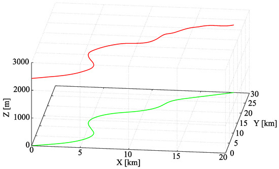
Figure 6.
Exemplary trajectory.
7.1. Ideal Atmospheric Conditions
To investigate the extended LQR control stability and tracking accuracy during long lasting flights, a scenario with no environmental perturbations was evaluated first. For this purpose, the local errors of states were examined. In Figure 7 output tracking errors are shown.
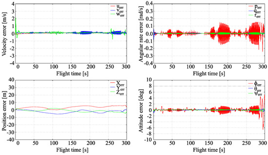
Figure 7.
Full tracking errors, quiet atmosphere.
The flight is stable and it can be seen that the output tracking is very accurate in the considered case. The local errors are low (roughly a few percent of the nominal values) and roughly uniform for over all the flight time, even these of the unobserved states . It can be stated that linear velocity errors are quite small, being of order 0.1–0.5 m/s. The position errors are less than ten meters at the end of flight, what is possible only if velocity errors are small enough. Considerable oscillations, which are of order 5 deg/s, are observed in roll angular rate p which is not measured. However, other states that are not measured () do not exhibit such behaviour. Oscillations of measured roll angle , attaining almost two degrees, are a consequence of roll rate oscillations. Pitch and yaw angle errors are very small, generally up to one degree over all the flight time. No significant oscillations of them are observed.
The LQR generated controls (control surfaces deflections) match good those that were recorded in flight, as can be seen in Figure 8. The elevator and rudder deflections match well the recorded values whereas computed deflections of aileron, although also close to recorded values, exhibits some oscillations. This coincides with oscillations of roll angular velocity p and roll angle .
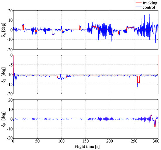
Figure 8.
Control errors.
The reasons of roll rate oscillations are not clear. They cannot be attributed fully to the lack of its measurement, because other not measured states do not exhibit oscillations. It is thus a suspicion that its origin lies in improper tuning of Q matrix that results in middle instability of the nonlinear closed loop system (aircraft-LQR controller).
Comparing to the similar results obtained for full state tracking with LQR [6], one can conclude that the overall stability and sensitivity of the output tracking problem with assumed measurements, although degraded to some extent (which was expected) does not significantly loose its ability to accurately track the prescribed flight path.
In a conclusion, results described above indicate that the generalized LQR control used for output tracking problem is stable. Moreover, it provides accurate tracking for the given path in the absence of external perturbations e.g., due to atmospheric conditions.
7.2. Influence of Atmospheric Disturbances
To investigate the robustness of the extended LQR control in an output-tracking problem, the influence of disturbances was examined. There are two types of disturbances: modelling and physical ones. Modelling errors are considered as exogenous disturbances [40] and are assumed neglectable, because the aircraft model was identified with high fidelity. Physical disturbances are caused by atmospheric phenomena, such as wind or turbulence. The perturbations concern both state and environment and they are usually diverse. Typical errors of disturbances are presented in Table 2.
Table 2.
Typical measurement errors in of nominal values percentage [6].
The first test concerns checking the robustness of LQR control with respect to constant disturbances. Steady horizontal right-side wind with velocity 5 m/s was introduced. No turbulence has been added. Results are presented in Figure 9.
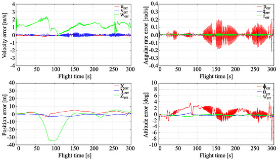
Figure 9.
Full tracking errors, wind presence.
There are no significant changes in LQR control efficiency when compared to outcomes presented in testing it with no disturbances. Increasing the wind velocity results in an approximately proportional decrease in tracking accuracy. The aircraft stability was affected only moderately. The selective oscillations of the roll rate and roll angle can be observed. Higher vertical velocity error and the Z coordinate error are caused by the changes in flight conditions introduced by wind that was not present in recorded flight. However, too high wind velocity or its adverse direction (tail wind), destroy stability and tracking completely and causes quick departure of an aircraft from the prescribed flight path. Maximal level of wind velocity that does not destroy tracking depends strongly on its direction and is roughly 20 m/s for head wind, 10 m/s for side wind and 5 m/s for tail wind.
The control errors are presented in Figure 10. It can be seen that the controls computed by LQR are less accurate when compared to the recorded ones. This is caused by the wind influence that was not present in recorded of flight. Higher level of aileron oscillations comparing to that of undisturbed case may also be observed.
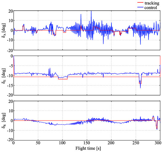
Figure 10.
Controls errors, wind presence.
In conclusion, it can be stated that steady wind does not cause a significant change in tracking accuracy and aircraft flight stability. Therefore the LQR control used in the output-tracking problem is robust enough with respect to the constant disturbances of moderate level.
The second test concerns checking the LQR control robustness regarding the stochastic type perturbations. Random turbulence with zero mean and variance proportional to velocity components in Table 2 was added to the measurement vector y. Wind has not been added in this test. Results are presented in Figure 11.
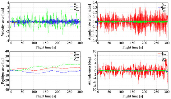
Figure 11.
Full tracking errors, turbulent conditions.
As in the previous test with steady wind, there are no significant changes in LQR control efficiency when compared to the outcomes shown in testing it with no disturbances. The main difference is that oscillations are present in all states. Oscillations of the roll rate and roll angle are higher than those of other states. Increasing the intensity of turbulence results in roughly proportional increasing oscillations of states, but tracking accuracy and aircraft flight stability was affected only moderately. However, too-high level of turbulence intensity destroys stability and tracking completely and causes quick departure of an aircraft from the flight path. The maximal level of turbulence intensity that did not destroy tracking was of order 3 m/s.
The controls computed by LQR are presented in Figure 12. It can be seen that they are largely distorted comparing to the recorded ones, although their mean values are close to these recorded in flight with no turbulence. A higher level of aileron oscillations is present compared to that of the undisturbed case. It is worth of notice, however, that oscillations of control computed by LQR are usually quite significant, even for problems with smooth states.
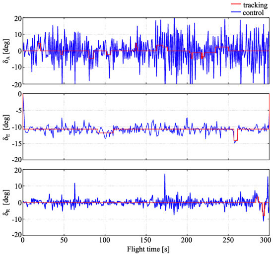
Figure 12.
Controls errors, turbulent conditions.
In conclusion, it can be stated that moderate turbulence does not cause a significant distortion of tracking accuracy as well as stability of aircraft flight. Therefore, it can be concluded that the LQR control used in output tracking problem is sufficiently robust with respect to stochastic type disturbances with zero mean values.
8. Conclusions
In this paper, an LQR controller was designed for an aircraft-tracking problem when some states were not observed. The controller design was based on a nonlinear aircraft model obtained from system identification when measurement and process noise was present in the data. The time domain filter error method based on the maximum likelihood principle allowed us to obtain accurate estimates of aerodynamic derivatives and the model had good predicting capabilities.
It has been shown that the LQR control can be used for handling of aircraft output tracking problem. The design was robust enough with respect to disturbances of moderate level. Even in the case of incomplete and inaccurate measurements, the output LQR controller has the ability of stable tracking the flight trajectory with quit good precision. Such abilities of the LQR depend essentially on the number and types of measured states. Too-poor measurements result in destabilizing the aircraft motion. The tracking accuracy decreases also because environment parameters were not estimated and thus not included in the LQR controller design.
In case of ideal atmospheric conditions, the aircraft tracking was sufficiently accurate and the local errors were small. This was true also for the unobserved states, with roll rate exception, for which considerable oscillations were observed. The LQR generated controls were in good agreement with their reference values. If the wind was added, the tracking accuracy dropped proportionally to the wind velocity. The LQR generated controls did not match reference values because the wind was not present in the reference flight. The controller was found to be robust if the wind was not too strong and did not act in diverse directions. Similar conclusions were drawn when turbulence was present in the experiment. Increasing turbulence had a proportional effect on all state variables oscillations, but again it was possible to provide accurate tracking for small and moderate disturbances.
It was possible to obtain accurate tracking, i.a., because of the high quality of the system identification model. For the model estimated with lower fidelity, the tracking quality would drop. This would be even more visible in case of fewer states present in the LQR static output feedback as less information would be available and thus the inaccuracies of the estimates would have greater overall contribution.
The theory concerning linear systems with static output feedback does not deliver conditions for the existence of stabilizing gain matrix that are easy to be checked—it is still a big challenge. However, it is possible to propose such a matrix for specific systems, e.g., as in our case, where the gain matrix being the solution of a standard LQR problem (that is with state feedback) together with the dynamic system matrices A, B, C satisfies simple scalar inequalities.
A success in using LQR control for nonlinear output tracking problem depends essentially on using a high fidelity flight mechanics model that compensates unmodelled aircraft dynamics due to, e.g., uncertainties or excitations shape degradation. The output LQR control is a useful instrument in the estimation and tuning process of highly nonlinear aircraft models from flight data, e.g., for high fidelity full flight simulator certification.
Enhancing of accuracy or stability of the LQR output feedback control depends essentially on internal stability of the object and, even more, on the number and types of available measurements. The brand new idea in this article consists of using LQR weighting matrices Q and R in the first step of a truncated iteration used for computing the exact gain matrix for output feedback [43]. The possibility of using the more advanced algorithm of such type for further accuracy enhancing is currently investigated.
In future, we plan to investigate tracking accuracy degradation due to state unavailability, weighting matrices auto-tuning and compare the outcomes with the results obtained for nonlinear quadratic regulator. We expect that nonlinear quadratic regulator will improve the tracking accuracy and that decrease in information content stored in states measurements (e.g., related to their unavailability) will degrade the trajectory tracking. However, this needs to be verified through at least numerical simulations. The final step of this research is to verify the results through hardware in the loop simulations, followed by high-fidelity full flight simulator tests and, finally, experiments performed on true aircraft.
Author Contributions
Conceptualization, P.L. and F.D.; methodology, P.L. and F.D.; software, P.L. and F.D.; validation, P.L., F.D. and A.K.; formal analysis, A.K.; investigation, P.L. and F.D.; resources, P.L.; writing—original draft preparation, P.L., F.D. and A.K.; writing—review and editing, P.L., F.D. and A.K.; visualization, P.L.; supervision, P.L.; project administration, P.L.; funding acquisition, P.L. All authors have read and agreed to the published version of the manuscript.
Funding
This research received no external funding.
Acknowledgments
The authors would like to thank German Aerospace Center (DLR) for providing the BACM model.
Conflicts of Interest
The authors declare no conflict of interest.
Abbreviations
| a, b | state and control matrices elements |
| b, | wingspan and mean aerodynamic chord |
| i-th row of the dynamic system matrix B | |
| e | vector elements |
| i-th versor; e.g., etc. | |
| f, g | state and output vector functions |
| g | gravitational acceleration |
| h | H matrix elements |
| i | iteration index |
| k | drag polar coefficient |
| j-th column of the matrix | |
| m | mass |
| n, m, p | number of states, control and outputs |
| o, s | output feedback and state feedback |
| , , N | number of estimated model outputs, process noise variables and time points |
| p | probability density function |
| p, q, r | roll, pitch and yaw rate |
| dynamic pressure | |
| r | reference value |
| t, | time and time at k-th point |
| u, v, w | longitudinal, side and vertical velocity |
| u | control vector |
| x, y, z | state, output and measurement vector |
| horizontal tail arm | |
| initial state | |
| A, B, C | state, control and output matrices |
| , , | longitudinal, side and vertical force coefficients |
| , , | rolling, pitching and yawing moment coefficients |
| , | lift and drag coefficients |
| , , | lift, side-force and drag coefficients bias |
| , , | rolling, pitching and yawing moment coefficients bias |
| i-th force or moment coefficient change due to j-th flight parameter or control | |
| i-th force or moment coefficient change due to k-th flight parameter effect on j | |
| D | triangular matrix |
| F, G | process and measurement noise distribution matrices |
| H | auxliary matrix |
| I, | inertia matrix and its component about i axis when the object is rotated about j axis |
| J | cost function |
| , | root mean square match and Theil inequality coefficient |
| gain matrix in LQR problem with state feedback | |
| optimal gain matrix in LQR problem with state feedback | |
| gain matrix in LQR problem with output feedback | |
| optimal gain matrix in LQR problem with output feedback | |
| stabilizing gain matrix in LQR problem with output feedback derived from | |
| M, S | gradient and auxiliary vector |
| P | state prediction error covariance matrix |
| unknown matrix in Riccati equation of LQR problem with state feedback | |
| matrix solving Riccati equation of LQR problem with state feedback | |
| unknown matrices in nonlinear equations describing optimal solution | |
| of LQR problem with output feedback | |
| matrices solving nonlinear equations describing optimal solution | |
| of LQR problem with output feedback | |
| Q, R | state and control weighting matrices |
| R | parameter error covariance matrix |
| real line | |
| , | output and control spaces |
| S, | wing area and horizontal tail area |
| T | thrust force |
| W | weighting factor matrix |
| , | linear and angular velocity |
| Z | indices of state coordinates present in the output vector |
| , | angle of attack and sideslip angle |
| , , | aileron, elevator and rudder deflection |
| time derivative of the variable | |
| vector estimates | |
| vector prediction | |
| control law for state feedback system | |
| control law for output feedback system | |
| , w | process and measurement noise |
| air density | |
| relative standard deviation | |
| , , | roll, pitch and yaw angle |
| Z set characteristic function | |
| , | unknown parameters and unknown system parameters |
| , | momentum and angular momentum |
| , | Fisher information and gradient matrices |
| , E | Hamiltonian and eigenvectors matrix |
| H | horizontal tail |
| wing body | |
| * | solution (optimal or of a set of equations) |
References
- Pawełek, A.; Lichota, P.; Dalmau, R.; Prats, X. Fuel-Efficient Trajectories Traffic Synchronization. J. Aircr. 2019, 56, 481–492. [Google Scholar] [CrossRef]
- Núñez, H.E.; MoraCamino, F.; Bouadi, H. Towards 4D Trajectory Tracking for Transport Aircraft. In Proceedings of the 20th IFAC World Congress, Toulouse, France, 9–14 July 2017. [Google Scholar] [CrossRef]
- Dalmau, R.; Pérez-Batlle, M.; Prats, X. Real-time Identification of Guidance Modes in Aircraft Descents Using Surveillace Data. In Proceedings of the 2018 IEEE/AIAA 37th Digital Avionics Systems Conference, London, UK, 23–27 September 2018. [Google Scholar] [CrossRef]
- Deori, L.; Garatti, S.; Prandini, M. 4-D Flight Trajectory Tracking: A Receding Horizon Approach Integrating Feedback Linearization and Scenario Optimization. IEEE Trans. Control Syst. Technol. 2019, 27, 981–996. [Google Scholar] [CrossRef]
- Emami, S.A.; Banazadeh, A. Intelligent trajectory tracking of an aircraft in the presence of internal and external disturbances. Int. J. Robust Nonlinear Control 2019, 29, 5820–5844. [Google Scholar] [CrossRef]
- Dul, F.A.; Lichota, P.; Rusowicz, A. Generalized Linear Quadratic Control for a Full Tracking Problem in Aviation. Sensors 2020, 20, 2955. [Google Scholar] [CrossRef]
- Wang, X.; Sang, Y.; Zhou, G. Combining Stable Inversion and H∞ Synthesis for Trajectory Tracking and Disturbance Rejection Control of Civil Aircraft Autolanding. Appl. Sci. 2020, 10, 1224. [Google Scholar] [CrossRef]
- Mortazavi, M.R.; Naghash, A. Pitch and flight path controller design for F-16 aircraft using combination of LQR and EA techniques. Proc. Inst. Mech. Eng. Part G J. Aerosp. Eng. 2018, 232, 1831–1843. [Google Scholar] [CrossRef]
- Yu, M.; Gong, X.; Fan, G.; Zhang, Y. Trajectory Planning and Tracking for Carrier Aircraft-Tractor System Based on Autonomous and Cooperative Movement. Math. Probl. Eng. 2020, 2020, 6531984. [Google Scholar] [CrossRef]
- Yan, K.; Wu, Q.; Chen, M. LQR-Based Optimal Tracking Fault Tolerant Control for a Helicopter with Actuator Faults. In Proceedings of the 2018 IEEE 7th Data Driven Control and Learning Systems Conference, Enshi, China, 25–27 May 2018. [Google Scholar] [CrossRef]
- Kopyt, A.; Topczewski, S.; Zugaj, M.; Bibik, P. An automatic system for a helicopter autopilot performance evaluation. Aircr. Eng. Aerosp. Technol. 2019, 91, 880–885. [Google Scholar] [CrossRef]
- Suicmez, E.C.; Kutay, A.T. Attitude and Altitude Tracking of Hexacopter via LQR with Integral Action. In Proceedings of the 2017 International Conference on Unmanned Aircraft Systems, Miami, FL, USA, 13–16 June 2017. [Google Scholar] [CrossRef]
- Martins, L.; Cardeira, C.; Oliveira, P. Linear Quadratic Regulator for Trajectory Tracking of a Quadrotor. In Proceedings of the 21st IFAC Symposium on Automatic Control in Aerospace, Cranfield, UK, 27–30 August 2019. [Google Scholar] [CrossRef]
- Almutairi, S.H.; Aouf, N. Enhancing the Aircraft’s Stability and Controllability against Actuator Faults using Robust Flight Control. In Proceedings of the 2016 IEEE International Conference on Control and Robotics Engineering, Singapore, 2–4 April 2016. [Google Scholar] [CrossRef]
- Djurovic, Z.M.; Kovacevic, B.D. A sequential LQG approach to nonlinear tracking problem. Int. J. Syst. Sci. 2008, 39, 371–382. [Google Scholar] [CrossRef]
- Chrif, L.; Kadda, Z.M. Aircraft Control System Using LQG and LQR Controller with Optimal Estimation-Kalman Filter Design. Procedia Eng. 2013, 80, 245–247. [Google Scholar] [CrossRef]
- Tang, Y.R.; Xiao, X.; Li, Y. Nonlinear dynamic modeling and hybrid control design with dynamic compensator for a small-scale UAV quadrotor. Measurement 2017, 109, 51–64. [Google Scholar] [CrossRef]
- Liu, C.; Chen, W.H.; Andrews, J. Tracking control of small-scale helicopters using explicit nonlinear MPC augmented with disturbance observers. Control Eng. Pract. 2012, 20, 258–268. [Google Scholar] [CrossRef]
- Gros, S.; Quirynen, R.; Diehl, M. Aircraft control based on fast non-linear MPC & multiple-shooting. In Proceedings of the 2012 IEEE 51st IEEE Conference on Decision and Control, Maui, HI, USA, 10–13 December 2012; pp. 1142–1147. [Google Scholar] [CrossRef]
- Fnadi, M.; Plumet, F.; Benamar, F. Model Predictive Control based Dynamic Path Tracking of a Four-Wheel Steering Mobile Robot. In Proceedings of the 2019 IEEE/RSJ International Conference on Intelligent Robots and Systems, Macau, China, 3–8 November 2019; pp. 4518–4523. [Google Scholar] [CrossRef]
- Klein, V. Estimation of aircraft aerodynamic parameters from flight data. Prog. Aerosp. Sci. 1989, 26, 1–77. [Google Scholar] [CrossRef]
- Deiler, C. Aerodynamic Modeling, System Identification, and Analysis of Iced Aircraft Configurations. J. Aircr. 2017, 55, 145–161. [Google Scholar] [CrossRef]
- Gross, M.; Costello, M. Smart Projectile Parameter Estimation Using Meta-Optimization. J. Spacecr. Rocket. 2019, 56, 1508–1519. [Google Scholar] [CrossRef]
- Simmons, B.M.; McClelland, H.G.; Woolsey, C.A. Nonlinear Model Identification Methodology for Small, Fixed-Wing, Unmanned Aircraft. J. Aircr. 2019, 56, 1056–1067. [Google Scholar] [CrossRef]
- Grauer, J.A. Real-Time Data-Compatibility Analysis Using Output-Error Parameter Estimation. J. Aircr. 2015, 52, 940–947. [Google Scholar] [CrossRef]
- Lu, H.H.; Rogers, C.; Goecks, V.G.; Valasek, J. Online Near Real Time System Identification on a Fixed-Wing Small Unmanned Air Vehicle. In Proceedings of the 2018 AIAA Atmospheric Flight Mechanics Conference, Kissimmee, FL, USA, 8–12 January 2018. [Google Scholar] [CrossRef]
- Valasek, J.; Chen, W. Observer/Kalman Filter Identification for Online System Identification of Aircraft. J. Guid. Control Dyn. 2003, 26, 347–353. [Google Scholar] [CrossRef]
- Borobia, R.; Sanchez-Arriaga, G.; Serino, A.; Schmehl, R. Flight-Path Reconstruction and Flight Test of Four-Line Power Kites. J. Guid. Control Dyn. 2018, 41, 2604–2614. [Google Scholar] [CrossRef]
- Shen, J.; Su, Y.; Liang, Q.; Zhu, X. Calculation and Identification of the Aerodynamic Parameters for Small-Scaled Fixed-Wing UAVs. Sensors 2018, 18, 206. [Google Scholar] [CrossRef]
- Seo, G.; Kim, Y.; Saderla, S. Kalman-filter based online system identification of fixed-wing aircraft in upset condition. Aerosp. Sci. Technol. 2019, 89, 307–317. [Google Scholar] [CrossRef]
- Chowdhary, G.; Jategaonkar, R.V. Aerodynamic parameter estimation from flight data applying extended and unscented Kalman filter. Aerosp. Sci. Technol. 2010, 14, 106–117. [Google Scholar] [CrossRef]
- Jategaonkar, R.V. Flight Vehicle System Identification: A Time Domain Methodology, 2nd ed.; Progress in Astronautics and Aeronautics; AIAA: Reston, VA, USA, 2015. [Google Scholar] [CrossRef]
- Fnadi, M.; Plumet, F.; Benamar, F. Nonlinear Tire Cornering Stiffness Observer for a Double Steering Off-Road Mobile Robot. In Proceedings of the 2019 International Conference on Robotics and Automation, Montreal, QC, Canada, 20–24 May 2019; pp. 7529–7534. [Google Scholar] [CrossRef]
- Deiler, C.; Fezans, N. VIRTTAC—A Family of Virtual Test Aircraft for Use in Flight Mechanics and GNC Benchmarks. In Proceedings of the AIAA Scitech 2019 Forum, San Diego, CA, USA, 7–11 January 2019. [Google Scholar] [CrossRef]
- Lichota, P.; Szulczyk, J.; Tischler, M.B.; Berger, T. Frequency Responses Identification from Multi-Axis Maneuver with Simultaneous Multisine Inputs. J. Guid. Control Dyn. 2019, 42, 2550–2556. [Google Scholar] [CrossRef]
- Cook, M.V. Flight Dynamics Principles, 3rd ed.; Elsevier: Amsterdam, The Netherlands, 2013. [Google Scholar] [CrossRef]
- Lichota, P.; Sibilski, K.; Ohme, P. D-Optimal Simultaneous Multistep Excitations for Aircraft Parameter Estimation. J. Aircr. 2017, 54, 747–758. [Google Scholar] [CrossRef]
- Hoak, D.E.; Finck, R.D. The USAF Stability and Control DATCOM; Technical Report TR-83-3048; Air Force Wright Aeronautical Laboratories: Dayton, OH, USA, 1978. [Google Scholar]
- Tischler, M.B.; Remple, R.K. Aircraft and Rotorcraft System Identification, 2nd ed.; AIAA Education Series; AIAA: Reston, VA, USA, 2012. [Google Scholar] [CrossRef]
- Skogestad, S.; Postlethwaite, I. Multivariable Feedback Control: Analysis and Design, 2nd ed.; Wiley: Hoboken, NJ, USA, 2005. [Google Scholar]
- Grimble, M.J. Robust Industrial Control Systems: Optimal Design Approach for Polynomial Systems, 1st ed.; Wiley: Chichester, UK, 2006. [Google Scholar]
- Stevens, B.L.; Lewis, F.L.; Johnson, E.N. Aircraft Control and Simulation, 3rd ed.; Wiley: Hoboken, NJ, USA, 2016. [Google Scholar]
- Kučera, V.; De Souza, C.E. A necessary and sufficient condition for output feedback stabilizability. Automatica 1995, 31, 1357–1359. [Google Scholar] [CrossRef]
- Kwakernaak, H.; Sivan, R. Linear Optimal Control Systems; John Wiley & Sons, Inc.: New York, NY, USA, 1972. [Google Scholar]
- Levine, W.S.; Athans, M. On the Determination of the Optimal Constant Output Feedback Gains for Linear Multivariable Systems. IEEE Trans. Autom. Control 1970, AC-15, 44–48. [Google Scholar] [CrossRef]
- Syrmos, V.L.; Abdallah, C.T.; Dorato, P.; Grigoriadis, K. Static output feedback—A survey. Automatica 1997, 33, 125–137. [Google Scholar] [CrossRef]
- Blondel, V.; Tsitsiklis, J. A survey of computational complexity results in systems and control. Automatica 2000, 36, 1249–1274. [Google Scholar] [CrossRef]
- Sadabadi, M.S.; Peaucelle, D. From static output feedback to structured robust static output feedback: A survey. Annu. Rev. Control 2016, 42, 11–26. [Google Scholar] [CrossRef]
- Moerder, D.D.; Calise, A.J. Convergence of a Numerical Algorithm for Calculating Optimal Output Feedback Gains. IEEE Trans. Autom. Control 1985, 30, 900–903. [Google Scholar] [CrossRef]
- Horn, R.A.; Johnson, C.R. Matrix Analysis, 2nd ed.; Cambridge University Press: New York, NY, USA, 2012. [Google Scholar]
- Karbowski, A. Optimal control of single retention reservoir during flood: Solution of deterministic, continuous-time problems. J. Optim. Theory Appl. 1991, 69, 55–81. [Google Scholar] [CrossRef]
- Karbowski, A. Shooting Methods to Solve Optimal Control Problems with State and Mixed Control-State Constraints. In Challenges in Automation, Robotics and Measurement Techniques; Szewczyk, R., Zielinski, C., Kaliczynska, M., Eds.; Advances in Intelligent Systems and Computing; Springer: Cham, Switzerland, 2016; Volume 440, pp. 189–205. [Google Scholar] [CrossRef]
Publisher’s Note: MDPI stays neutral with regard to jurisdictional claims in published maps and institutional affiliations. |
© 2020 by the authors. Licensee MDPI, Basel, Switzerland. This article is an open access article distributed under the terms and conditions of the Creative Commons Attribution (CC BY) license (http://creativecommons.org/licenses/by/4.0/).