Design and 3D CFD Static Performance Study of a Two-Blade IceWind Turbine

Abstract

The IceWind turbine, a new type of Vertical Axis Wind Turbine, was proposed by an Iceland based startup. It is a product that has been featured in few published scientific research studies. This paper investigates the IceWind turbine’s performance numerically. Three-dimensional numerical simulations are conducted for the full scale model using the SST K-ω model at a wind speed of 15.8 m/s. The following results are documented: static torque, velocity distributions and streamlines, and pressure distribution. Comparisons with previous data are established. Additionally, comparisons with the Savonius wind turbine in the same swept area are conducted to determine how efficient the new type of turbine is. The IceWind turbine shows a similar level of performance with slightly higher static torque values. Vortices behind the IceWind turbine are confirmed to be three-dimensional and are larger than those of Savonius turbine.

1. Introduction

Many factors have led to increased interest in renewable energy including the reduction in conventional energy sources, the fact that conventional energy sources cause climate change, and the availability and hygiene of renewable energy sources. Lately, wind energy has become particularly important. The IceWind turbine is a new type of Vertical Axis Wind Turbine (VAWT) that converts wind energy into electricity. It is an attractive and cost effective energy source for electric generation in low velocity regions. The prefix “Ice” in “IceWind” comes from “Iceland”, its home town [1]. Currently, there are two products: the CW IceWind turbine, shown in Figure 1, and the RW IceWind turbine, shown in Figure 2.

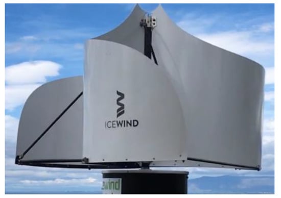
Figure 1. CW IceWind turbine.

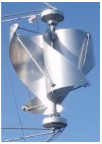
Figure 2. RW IceWind turbine.

The IceWind turbine was first introduced by Aymane [2]. He mentioned that the IceWind turbine is not as simple to manufacture as the Savonius wind turbine, but its shape is better looking. Furthermore, the IceWind turbine produces less noise than the Savonius turbine. He confirmed that any product should not only show a good level of performance but should also have wide acceptance from the public. He invited participants to fill in a survey about the overall appearance, noise level, and efficiency of the turbine. Eighty-five percent of participants declared that the IceWind turbine produced less noise and had a better overall appearance than the Barrel Savonius. Moreover, Afify [3] investigated the turbine’s performance experimentally to determine its optimum design. He concluded that a single stage, three-blade IceWind turbine with end plates, an aspect ratio of 0.38, and a blade arc angle of 112° performs better than the Savonius turbine.

Computational Fluid Dynamics (CFD) can predict fluid flow aerodynamic performance. Sarma et al. [4] mentioned that the intent of using CFD is to enable the study of velocity and torque distribution. Nasef et al. [5] numerically analyzed the aerodynamic performance of stationary and rotating Savonius rotors with several overlap ratios using four turbulence models. Their results indicated that the Shear Stress Transport (SST) k-ω turbulence model gives more accurate results than the other studied turbulence models. Kacprzak et al. [6] examined the performance of the Savonius wind turbine with fixed cross-sections using quasi 2D flow predictions through ANSYS CFX. Simulations were achieved in a way that allowed comparison with wind tunnel data documented in a related paper, where two designs were simulated: Classical and Bach-type Savonius rotors. The comparison detected the significance of applying a laminar-turbulent transition model. Dobrev and Massouh [7] aimed to consider the flow through a Savonius type turbine using a three-dimensional model by means of k-ω and DES (Detached Eddy Simulation). Due to the continuous variation of the flow angle with respect to the blades and turbine principles of operation, strong unsteady effects including separation and vortex shedding were observed. The flow analysis helped to validate their wind turbine design. McTavish et al. [8] developed a novel vertical axis wind turbine (VAWT) consisting of many asymmetric vertically stacked stages. The VAWT torque characteristics were computationally investigated using CFdesign 2010 software. Steady two-dimensional CFD simulations demonstrated that the new type had similar average static torque characteristics to present Savonius rotors. Additionally, rotating three-dimensional CFD simulations were performed.

In the present study, three-dimensional numerical simulations are used to calculate the static torque of the IceWind turbine and to show its air flow velocity distribution and streamlines and pressure distribution.

2. Physical Model

Figure 3 shows the steps used in SolidWorks to draw the IceWind blade. It consists of three circles and three lines arranged as shown in Figure 3a. Trimming was used and dimensions were applied, as shown in Figure 3b. The sketch was revolved 90° about its axis (right vertical line), as shown in Figure 3c, and then, the extrude function was used to cut the shape, as shown in Figure 3d. Figure 4 shows the final IceWind blade that was used in this study. Its dimensions are d = 75 mm and H = 75 mm with a 25 mm blade tip height and a swept area of A_s = 4250.51 mm². Figure 5 and Figure 6 show the used IceWind turbine.

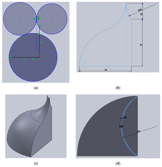
Figure 3. Steps used in SolidWorks to draw the IceWind blade (dimensions are in mm). (a) First shape; (b) trimmed shape; (c) revolved shape; (d) preparation of extruded cut shape.

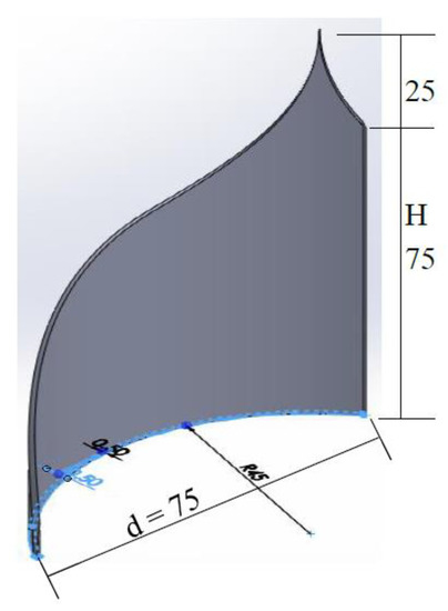
Figure 4. IceWind blade (dimensions are in mm).

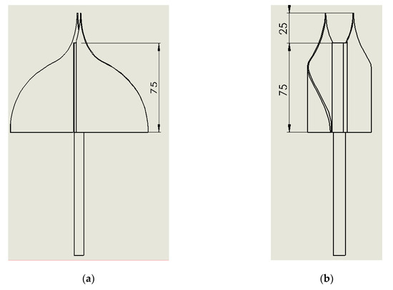
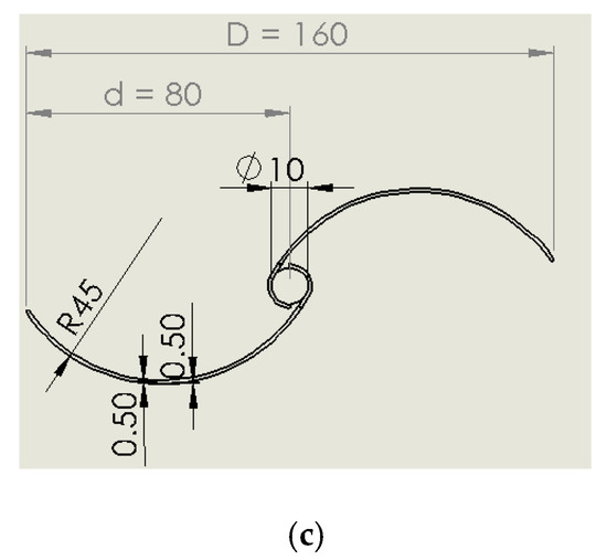
Figure 5. IceWind turbine’s three views (dimensions are in mm): (a) elevation, (b) side view, and (c) plan.

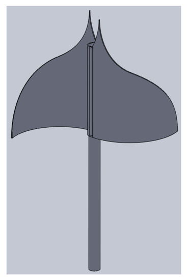
Figure 6. IceWind turbine.

3. Numerical Model

Simulations of air flow around the turbine were conducted using Ansys FLUENT after setting the test conditions to be similar to real conditions.

3.1. Domain Dimensions

The numerical domain included the wind tunnel space and the IceWind turbine, as shown in Figure 7, to simulate the flow around the turbine. The upstream, downstream, width, and height dimensions were 500, 500, 300, and 300 mm, respectively, as shown in Figure 7. The domain’s overall dimensions were 300 × 300 × 1000 mm. These dimensions are the wind tunnel and turbine dimensions given in [3].

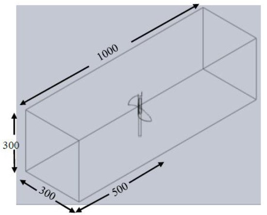
Figure 7. Wind tunnel space with the IceWind turbine and domain dimensions (mm).

A position angle θ was defined as the angle where the blade tips were inclined to the direction of the wind tunnel’s air flow, as shown in Figure 8.

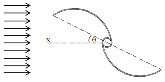
Figure 8. A position angle θ of the turbine’s two blades.

3.2. Boundary Conditions

The boundary conditions are shown in Figure 9 and Table 1. They are exactly as used in [3]. The left boundary was defined as an inlet. The air flow was a wind velocity of 15.8 m/s. A pressure outlet boundary condition was assumed at the right boundary. Other boundaries and the turbine were considered to be walls.

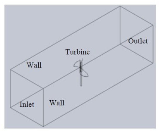
Figure 9. Boundary conditions.

Table 1. Boundary conditions.

Boundary Location	Boundary Condition
Inlet (Left)	Velocity inlet
Outlet (Right)	Pressure outlet
Top	Wall
Sides	Wall
bottom	Wall
Turbine’s surfaces	Wall

3.3. Domain Meshing

The accuracy of the model results was sensitive to the size and distributions of the mesh. For this three-dimensional simulation study, two diverse zones—the rotating and stationary zones—were drawn. A vertical cylinder around the turbine was considered to be the rotating zone, and the whole wind tunnel test section excluding this cylinder was the stationary zone, as shown in Figure 10.

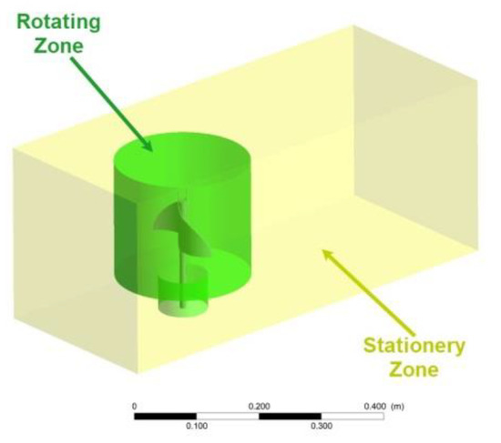
Figure 10. Two different zones of the IceWind turbine’s domain: rotating and stationary zones.

A mesh independency study was carried out. Figure 11 shows the relation between static torque and the number of elements at an air velocity of 15.8 m/s for the IceWind turbine at θ = 90°. For element numbers of 4.5 × 10⁶ and 7.8 × 10⁶, the value of static torque (N·m) was almost the same. To give a high level of accuracy, 7.8 × 10⁶ elements were used.

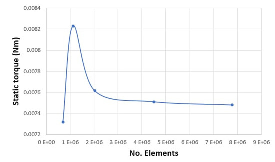
Figure 11. Relation between static torque and the number of elements at an air velocity of 15.8 m/s for the IceWind turbine at θ = 90°.

Figure 12 and Figure 13 show that computational mesh consists of tetrahedral cells. It is very fine around the blades and shaft (maximum ${\mathrm{y}}^{+}$ below 2). A close-to-equilateral coarse mesh is generated in the stationary zone. The contact between these two zones is considered to be the interface boundary condition, and this guarantees that continuity in the flow field is acquired while minimizing numerical errors. Second order discretization was used for all solution variables [9].

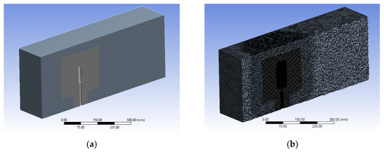
Figure 12. Mesh of the IceWind turbine domain (section): (a) elevation and (b) side view.

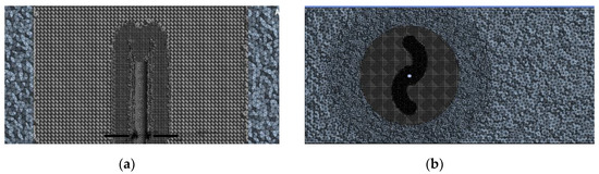
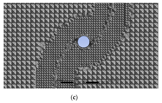
Figure 13. Mesh of the IceWind turbine domain (zoomed in): (a) elevation, (b) plan, and (c) plan (zoomed in).

3.4. Turbulence Modeling Approach

The regime of the system was laminar. Previous studies showed that the k-ε and Spallart-Allmaras models cannot catch and predict the flow progress, especially in the laminar separation bubble [10,11]. Therefore, the SST k-ω model [12,13] can be utilized as a low Reynolds turbulence model with no additional damping functions. Shear Stress Transport (SST) formulation is created by combining the k-ω and k-ε models. This structure supports the use of the SST method to switch to the k-ε model to revoke the problems of k-ω in inlet free-stream turbulence properties and utilize the k-ω formulation in the internal parts of the boundary layer. The k-ω SST model is a commonly used turbulent model in VAWT simulations [14,15,16,17,18,19,20]. Furthermore, it is a good predictor of turbulence in adverse pressure gradients and separating flow.

Two mathematical formulas, k and ω equations, are proposed for use in SST methods below [9]:

$$\frac{\partial \left(\rho k\right)}{\partial t}+\frac{\partial \left(\rho k{u}_i\right)}{\partial x_i}=\frac{\partial }{\partial x_j}\left({\mathsf{\Gamma }}_k\frac{\partial k}{\partial x_j}\right)+G_k-Y_k+s_k$$

(1)

$$\frac{\partial \left(\rho \omega \right)}{\partial t}+\frac{\partial \left(\rho \omega u_i\right)}{\partial x_i}=\frac{\partial }{\partial x_j}\left({\mathsf{\Gamma }}_{\omega }\frac{\partial \omega }{\partial x_j}\right)+G_{\omega }-Y_{\omega }+s_{\omega }$$

(2)

where ${\mathsf{\Gamma }}_k$ and ${\mathsf{\Gamma }}_{\omega }$ express the active diffusivity of k and ω. s_k and s_ω are user-defined source terms. G_k and G_ω show the turbulent kinetic energy generation due to the mean velocity gradients. Y_k and Y_ω mean the dissipation of k and ω due to turbulence.

The chosen fluid model for computation comprises air at 25 °C, pressure equal to one atmosphere, isothermal heat transfer, and a turbulent flow model.

For laminar steady flow, the simulations were run to reach steady state conditions, and the residuals reached a value of less than 6 × 10⁻⁵, as shown in Figure 14.

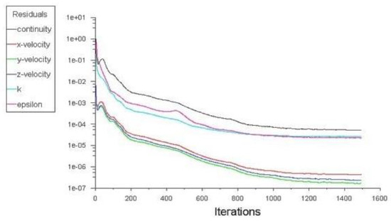
Figure 14. Relation between residuals and the number of iterations at an air velocity of 15.8 m/s for the IceWind turbine at θ = 90°.

4. Savonius Turbine

Due to the lack of visualization results for the IceWind turbine, the traditional turbine type was compared with the performance of the new type (IceWind turbine). To ensure a good assessment, the authors used the Savonius turbine, as shown in Figure 15 and Figure 16, with the same swept area: A_s = 4250.51 mm². With the same d value of 75 mm, the Savonius blade height was equal to 56.67 mm. To ensure consistency, all IceWind turbine three-dimensional simulation conditions were applied for the Savonius turbine, including the domain dimensions, domain meshing, and turbulence modeling approach.

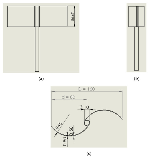
Figure 15. The Savonius turbine’s three views (dimensions are in mm): (a) elevation, (b) side view, and (c) plan.

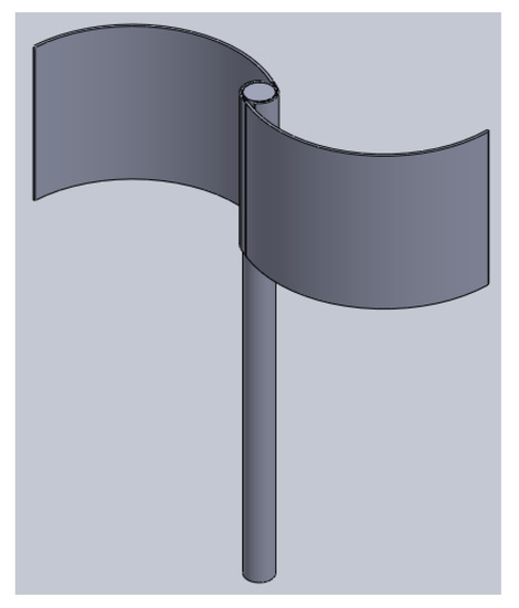
Figure 16. Savonius turbine.

5. Results

This considered case was a still rotor case. The tip speed ratio—tip speed divided by wind speed—was equal to zero because the rotor was fixed for each simulated angle.

Static torque—starting torque—is the torque required for starting turbine rotation. Figure 17 shows the relation between static torque and the rotation angle for the IceWind and Savonius turbines at an air velocity of 15.8 m/s. The static torque of the IceWind turbine was found to have two peaks at θ = 60° and 240°. The Savonius turbine also showed two peaks but not at the same angles. The IceWind and Savonius turbines reached maximum values of 0.055 and 0.052 N·m, respectively. These slight differences may be because the flow field is two-dimensional near the Savonius rotor, whereas near IceWind rotor, it is three-dimensional. This fact will be proved later in the present study. It was found that the torque performance is improved by the IceWind rotor shape.

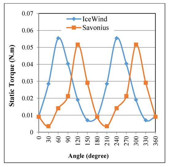
Figure 17. Relation between static torque and the rotation angle for the IceWind and Savonius turbines at an air velocity of 15.8 m/s.

Determination of the air flow velocity distribution and streamlines and pressure distribution around the turbine’s surface enabled the air flow characteristics, disturbances, and locations of the highest pressure to be found. The air velocity distribution and streamline and pressure distribution results for both turbines at a wind velocity of 15.8 m/s are shown in Figure 18, Figure 19 and Figure 20. The rotors of the two turbines showed similar flow patterns. The flow structure around the Savonius rotor was called “Coanda-like flow” by [21,22], and it controls flow separation on the convex side. A low pressure region forms on the side of the proceeding blade, contributing to the torque generation of the rotating rotor [23].

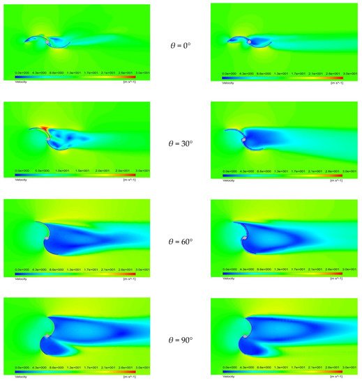
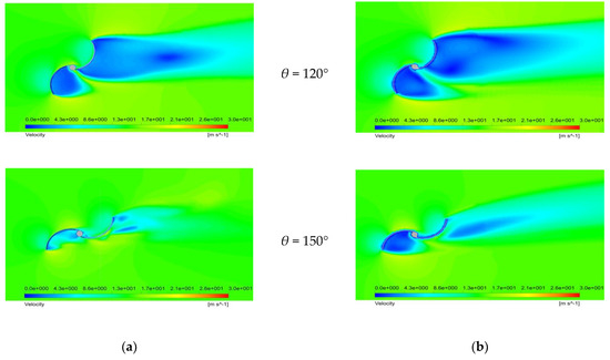
Figure 18. Air flow velocity distributions at an air velocity of 15.8 m/s around (a) the IceWind turbine and (b) the Savonius wind turbine.

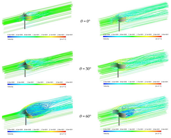
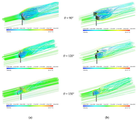
Figure 19. Air flow velocity streamlines at an air velocity of 15.8 m/s around (a) the IceWind turbine and (b) the Savonius wind turbine.

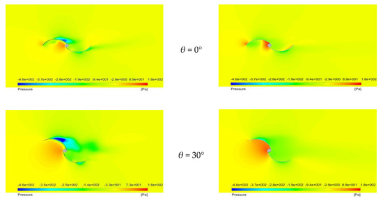
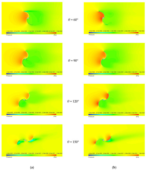
Figure 20. Pressure distributions at an air velocity of 15.8 m/s around (a) the IceWind turbine and (b) the Savonius wind turbine.

Figure 18a,b show the air flow velocity distribution around the still IceWind and Savonius turbines’ rotors. These results were obtained at the plane that goes through the bottom of the turbines’ blades as both have the same complete shape at this plane. The figures show similar velocity distributions. At θ = 0°, the high fluid flow velocity moves at a tangent to the convex sides, while two circulating low velocity zones in the two concave sides are established. The air flow velocity has a slightly different maximum velocity of 28 m/s for the IceWind turbine compared with 22 m/s for the Savonius turbine. At θ = 90°, the largest dead area is observed in the wake of the returning blade. The figures show similar velocity distributions. High fluid flow velocity touches the ends of both blades. Furthermore, a pair of asymmetric vortices develops behind both turbines. The smallest dead area is observed in the wake of the returning blade at θ = 0°. Moreover, a maximum velocity of 34 m/s is observed for the IceWind turbine at θ = 30°.

Figure 19a,b show air flow velocity streamlines around the still IceWind and Savonius turbines rotors at a velocity of 15.8 m/s. It is obvious from the figures that vortices behind the Savonius rotor are located between two imaginary planes that go through the top and bottom of the turbine blades. However, the rotor can be considered to be two-dimensional along the whole height. According to the top curvature of IceWind turbine, the plane that goes through the top of the turbine blades does not exist anymore. However, the plane that goes through the bottom of the turbine blades still exists. Vortices are located between the plane that goes through the bottom of the turbine blades and another inclined plane that follows the turbine top curvature. This provides IceWind turbine vortices with three-dimensionality. Vortices behind the IceWind turbine rotor appear to be larger than those behind the Savonius turbine.

Figure 20a,b show air flow pressure distributions around the still IceWind and Savonius turbines’ rotors. These results were obtained at the plane that goes through the bottom of the turbines’ blades as both have the same complete shape at this plane. The concave side of the proceeding blade has a positive pressure, while the convex side of the same blade has a negative pressure. In contrast, the concave side of the returning blade has a negative pressure, while the convex side of the same blade has a positive pressure. In other words, positive pressure appears on the turbine side facing the air, and the opposite sides have a negative pressure. At θ = 0°, both figures show similar pressure distributions. The dead area is small, and the vortex producing a negative pressure almost disappears, whereas the largest dead area is observed in the wake of the returning blade at θ = 90°. Separation occurs due to an adverse pressure gradient in the downstream direction. Both figures show similar pressure distributions. Moreover, the maximum negative pressure appears at θ = 30° for both turbines.

Three-dimensional numerical modeling was successfully used in the current case to visualize the flow around both turbines. This visualization comparison with the Savonius turbine showed noticeably similar performances for the two turbines.

6. Comparison with Previous Work

It would be better to use the coefficient of static torque than static torque for comparison, but in the present paper, the same outcome would have been achieved because the present study and [3] used the same dimensions and conditions.

Figure 21 shows the relation between static torque and the rotation angle at an air velocity of 15.8 m/s as determined in an experimental study [3] and in the present numerical study on the IceWind turbine. The same trend was observed. The static torque was found to have two peaks at θ = 60° and 240° in both studies. Moreover, the present numerical results gave slightly lower values than the experimental results. The IceWind turbine reached maximum values of 0.055 and 0.064 Nm for the numerical and experimental studies [3], respectively. This deviation may be due to the experimental conditions and numerical assumptions made.

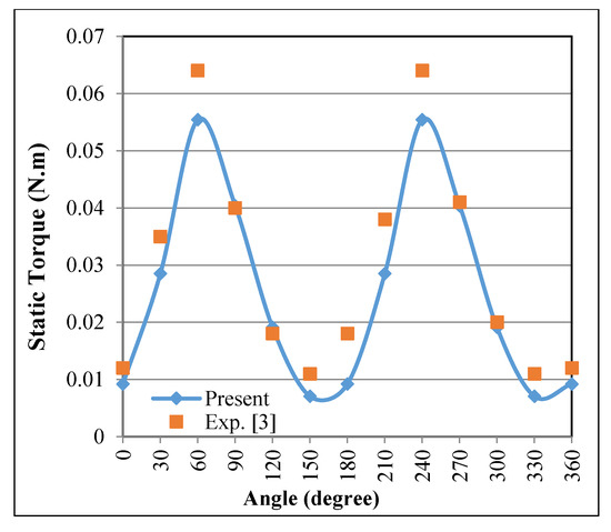
Figure 21. Relation between static torque and the rotation angle for the IceWind turbine at an air velocity of 15.8 m/s in the numerical and experimental [3] studies.

7. Conclusions

In the current work, three-dimensional simulations on a new Vertical Axis Wind Turbine type called the IceWind turbine were conducted. Ansys FLUENT was used to determine the static torque, velocity distributions and streamlines, and pressure distributions at a wind velocity of 15.8 m/s. From the numerical results, the following can be concluded:

• The comparison between the IceWind and Savonius turbines showed similar flow patterns. However, the IceWind turbine was found to be slightly better than the Savonius wind turbine with the same swept area. Although the IceWind turbine is not simple to manufacture, its shape has a better look and performance.
• The air flow velocity distribution of the IceWind turbine led to the maximal velocity and a larger wake area.
• The air flow velocity streamlines demonstrated that vortices behind the IceWind rotor are three-dimensional.
• The air flow pressure distributions showed that positive pressure appears on the turbine side facing the air. On the opposite side, the pressure is negative.
• The numerical method validated previous experimental works, and reasonable agreement was achieved.

References

- IceWind Turbine Site. Available online: http://icewind.is/en/ (accessed on 27 November 2019).
- Aymane, E. Savonius Vertical Wind Turbine: Design, Simulation, and Physical Testing. Master’s Thesis, School of Science and Engineering, Alakhawayn University, Ifrane, Morocco, 2017. [Google Scholar]
- Afify, R.S. Experimental Studies of an IceWind Turbine. Int. J. Appl. Eng. Res. 2019, 14, 3633–3645. [Google Scholar]
- Sarma, N.K.; Biswas, A.; Misra, R.D. Experimental and computational evaluation of Savonius hydrokinetic turbine for low velocity condition with comparison to Savonius wind turbine at the same input power. Energy Convers. Manag. 2014, 83, 88–98. [Google Scholar] [CrossRef]
- Nasef, M.H.; El-Askary, W.A.; AbdEL-hamid, A.A.; Gad, H.E. Evaluation of Savonius rotor performance: Static and dynamic studies. J. Wind Eng. Ind. Aerodyn. 2013, 123, 1–11. [Google Scholar] [CrossRef]
- Kacprzak, K.; Liskiewicz, G.; Sobczak, K. Numerical investigation of conventional and modified Savonius wind turbines. Renew. Energy 2013, 60, 578–585. [Google Scholar] [CrossRef]
- Dobrev, I.; Massouh, F. CFD and PIV investigation of unsteady flow through Savonius wind turbine. Energy Procedia 2011, 6, 711–720. [Google Scholar] [CrossRef]
- McTavish, S.; Feszty, D.; Sankar, T. Steady and rotating computational fluid dynamics simulations of a novel vertical axis wind turbine for small-scale power generation. Renew. Energy 2012, 41, 171–179. [Google Scholar] [CrossRef]
- Fluent, A. 12.0 Theory Guide; Ansys Inc.: Canonsburg, PA, USA, 2009. [Google Scholar]
- Marsh, P.; Ranmuthugala, D.; Penesis, I.; Thomas, G. Three-dimensional numerical simulations of straight-bladed vertical axis tidal turbines investigating power output, torque ripple and mounting forces. Renew. Energy 2015, 83, 67–77. [Google Scholar] [CrossRef]
- McNaughton, J.; Billard, F.; Revell, A. Turbulence modelling of low Reynolds number flow effects around a vertical axis turbine at a range of tip-speed ratios. J. Fluids Struct. 2014, 47, 124–138. [Google Scholar] [CrossRef]
- Wilcox, D.C. Turbulence Modeling for CFD, 2nd ed.; DCW Industries: La Canada Flintridge, CA, USA, 1998; ISBN 0-9636051-5-1. [Google Scholar]
- Blazek, J. Computational Fluid Dynamics: Principles and Applications, 1st ed.; Elsevier Science Ltd.: Oxford, UK, 2001; ISBN 0080430090. [Google Scholar]
- Menter, F.R. Two-equation eddy-viscosity turbulence models for engineering applications. AIAA J. 1994, 32, 1598–1605. [Google Scholar] [CrossRef]
- Chong, W.; Fazlizan, A.; Poh, S.; Pan, K.; Hew, W.; Hsiao, F. The design, simulation and testing of an urban vertical axis wind turbine with the Omni-direction-guide-vane. Appl. Energy 2013, 112, 601–609. [Google Scholar] [CrossRef]
- Nobile, R.; Vahdati, M.; Barlow, J.F.; Mewburn-Crook, A. Unsteady flow simulation of a vertical axis augmented wind turbine: A two-dimensional study. J. Wind Eng. Ind. Aerodyn. 2014, 125, 168–179. [Google Scholar] [CrossRef]
- Lim, Y.; Chong, W.; Hsiao, F. Performance investigation and optimization of a vertical axis wind turbine with the Omni-direction-guide-vane. Procedia Eng. 2013, 67, 59–69. [Google Scholar] [CrossRef]
- Danao, L.A.; Edwards, J.; Eboibi, O.; Howell, R. A numerical investigation into the influence of unsteady wind on the performance and aerodynamics of a vertical axis wind turbine. Appl. Energy 2014, 116, 111–124. [Google Scholar] [CrossRef]
- Mohamed, M.H.; Ali, A.M.; Hafiz, A.A. CFD analysis for H-rotor Darrieus turbine as a low speed wind energy converter. Eng. Sci. Technol. 2015, 18, 1–13. [Google Scholar] [CrossRef]
- Almohammadi, K.M.; Ingham, D.B.; Ma, L.; Pourkashan, M. Computational fluid dynamics (CFD) mesh independency techniques for a straight blade vertical axis wind turbine. Energy 2013, 58, 483–493. [Google Scholar] [CrossRef]
- Fujisawa, N.; Gotoh, F. Visualization study of the flow in and around a Savonius rotor. Exp. Fluids 1992, 12, 407–412. [Google Scholar] [CrossRef]
- Fujisawa, N. On the torque mechanism of Savonius rotors. J. Wind Eng. Ind. Aerodyn. 1992, 40, 277–292. [Google Scholar] [CrossRef]
- Fujisawa, N.; Gotoh, F. Pressure measurements and flow visualization study of a Savonius rotor. J. Wind Eng. Ind. Aerodyn. 1992, 39, 51–60. [Google Scholar] [CrossRef]
Publisher’s Note: MDPI stays neutral with regard to jurisdictional claims in published maps and institutional affiliations. |
© 2020 by the authors. Licensee MDPI, Basel, Switzerland. This article is an open access article distributed under the terms and conditions of the Creative Commons Attribution (CC BY) license (http://creativecommons.org/licenses/by/4.0/).