1. Introduction
In recent years, more and more attention has been devoted to ecology-based issues. They have been considered among the communities of different areas such as electrical, chemical, or mechanical engineering. In the area of lighting technique, the ecological trends have also been easily visible [
1,
2,
3,
4,
5,
6]. Within these trends, one of the problems taken into account by researchers is the problem of light pollution, which is associated with the lighting of outdoor areas. Initially, the presence of artificial lighting in public places was met with approval. Unfortunately, using the lighting on a mass scale showed has led to light pollution, which is a result of too many light sources installed in a limited space. Light pollution may be defined as a disturbance of the natural level of brightness of the nocturnal environment through artificial light sources installed by man. Light pollution is a very complex issue, and its complexity is confirmed by many works located in the various fields of science as astronomy, atmosphere physics, biology, ecology, medicine, and sociology [
1,
7,
8,
9,
10]. One of the forms of light pollution is the formation of a sky glow, which usually takes place over urban areas [
11]. During cloudiness, light reflects off the clouds, causing light pollution in areas located a distance away from the cities. The literature reports that, from the point of view of environmental protection, light pollution has a similar rank as emission to the environment solid, liquid, and gaseous pollutants. The presence of artificial light during the night has an important effect on the functioning of animals. It may disturb their daily, monthly, and yearly cycles. Light pollution may influence the foraging, migration, and communication of organisms in their natural environment [
12,
13,
14]. Staying in a contaminated environment can be a potential threat to mammals (including humans). Artificial light can interfere with the production of melatonin, a hormone with antioxidant and anti-cancerogenic effects [
15]. Light pollution has an adverse effect on flora and fauna. As a result of intense lighting, algae, in aquatic ecosystems, increases biomass production [
16]. It was also stated that, as a result of light pollution in suburban lakes, Daphnia shows smaller amplitude and size of migration and due to this fact algae are eaten less intensely at night [
12]. In reference [
17], the authors point out the special threat of the eutrophication of drinking water tanks due to light pollution, which is associated with a deterioration of water quality.
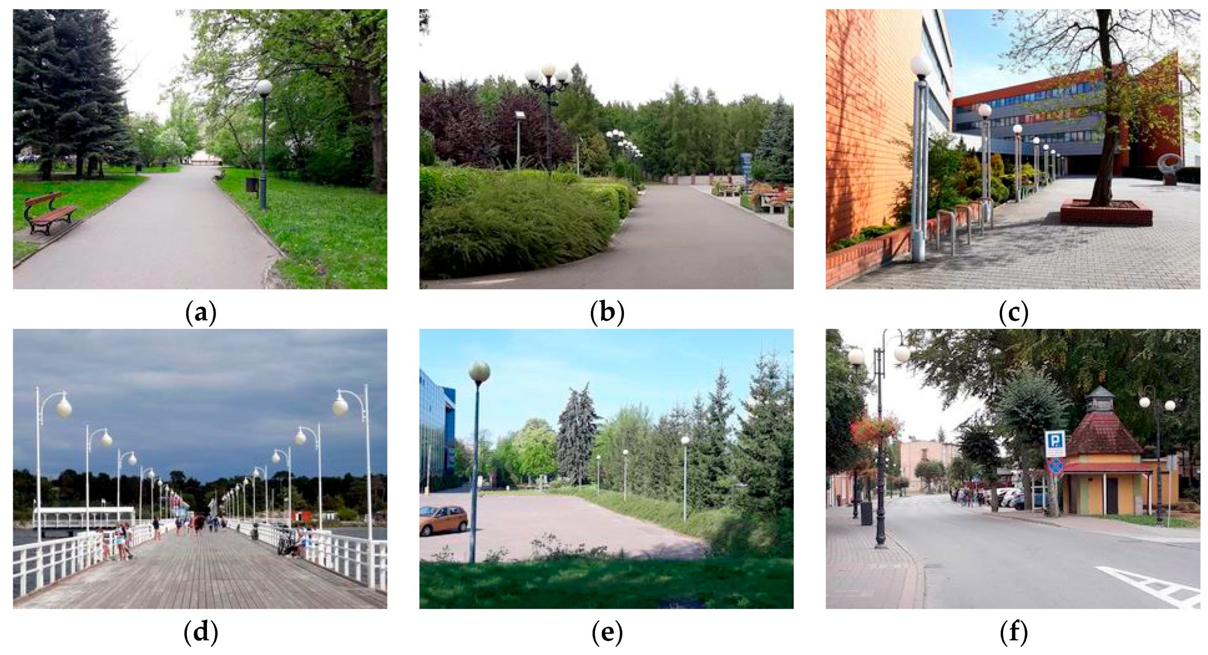
The areas where light pollution is easy to recognize are the green areas—for example parks, gardens, squares, or alleys. In these areas, lighting has two basic functions: functional and decorative [
5,
6,
18,
19,
20]. The purpose of functional lighting is to ensure safety for walkers; decorative lighting serves to emphasize the value of the surroundings (plants, objects, etc.). One of the commonly used lighting luminaries in urban infrastructure is an opal sphere type luminaire. It is used, among others, for illuminating park avenues (
Figure 1a), gardens (
Figure 1b), spaces in front of the buildings (
Figure 1c), piers (
Figure 1d), parking lots (
Figure 1e), and residential roads (
Figure 1f). Its popularity is a result of several factors such as simple design allowing easy access to the light source, possibility of fitting the luminaire in more than one type of light source, and low price.
The opal sphere type luminaires usually cooperate with high-pressure sodium lamps (HPSs) or metal halide lamps (MHs), although the design of the luminaire also allows it to be equipped with other light sources such as classic incandescent lamps (INCs), high-pressure mercury lamps (HPMs), integrated compact fluorescent lamps (CFLs), or induction lamps (ILs). Due to low luminous efficiency, the use of the light bulbs and mercury lamps is marginal. As a result of one of the priority actions of the European Union (EU), authorities are obligated to reduce electricity consumption, and an important branch of electricity, where this aspect is considered, is electric lighting. The effect of the actions made by the EU is a process of withdrawing energy-consuming light sources and promoting the introduction of modern light sources like light-emitting diodes (LEDs) [
4,
21,
22]. For this reason, LED sources are also considered as the light sources possible to be installed in the opal sphere type luminaries. Hence, it is worth noting that, due to various physical phenomena occurring in the generation of light in the individual light sources, the radiation produced by them will be different, which can have an impact on the phenomenon of light pollution. The consequence of equipping the luminaries with the light sources of different spectral power distribution (SPD) is a change in the way that light is distributed. Hence the way the light is distributed influences the light pollution effect.
In general, the number of works devoted to the influence of SPD on the effect of light pollution is significant [
11,
23,
24,
25,
26,
27,
28,
29,
30,
31,
32,
33]. Within these studies, there are many works in which analysis of the influence of SPD on light pollution effect is extended by consideration of spectral reflectance of the ground or atmosphere properties. One research group has also elaborated the advanced numerical model called ILLUMINA that allows for the simulation of the brightening of the night sky caused by the emission of artificial light by man [
30]. Due to the fact that opal sphere type luminaires are very popular and may work in principle with any light sources, the authors decided to make an analysis of the impact of various types of light sources on the effect of light pollution. Hence, in this paper the laboratory measurements and computer simulations were made, and the light sources selected were the sources of latest generation including LEDs as well as older-generation such as INCs. The laboratory measurements included the determination of the distribution of light emitted by the luminaire equipped with distinctive light sources as well as registration of the spectral characteristics of the radiation emitted by the luminaire. The results from the laboratory measurements were then used in the simulations based on the software supporting the lighting design process. The simulations were carried out for the same light sources as used in the laboratory studies and for two typical ways of installation of the light sources in the luminaire: with the handle down and the handle up. Within the simulation, we modelled a grassy ground with a single lantern standing at its center and equipped with opal sphere type luminaire. Due to the complexity of the problem, the introduction of a larger number of luminaires or lanterns as well as other objects such as trees or shrubs, was abandoned. However, the issue of the lantern’s location and degree of complexity of the analyzed area will be considered in the further works of the authors.
2. Methodology of the Studies
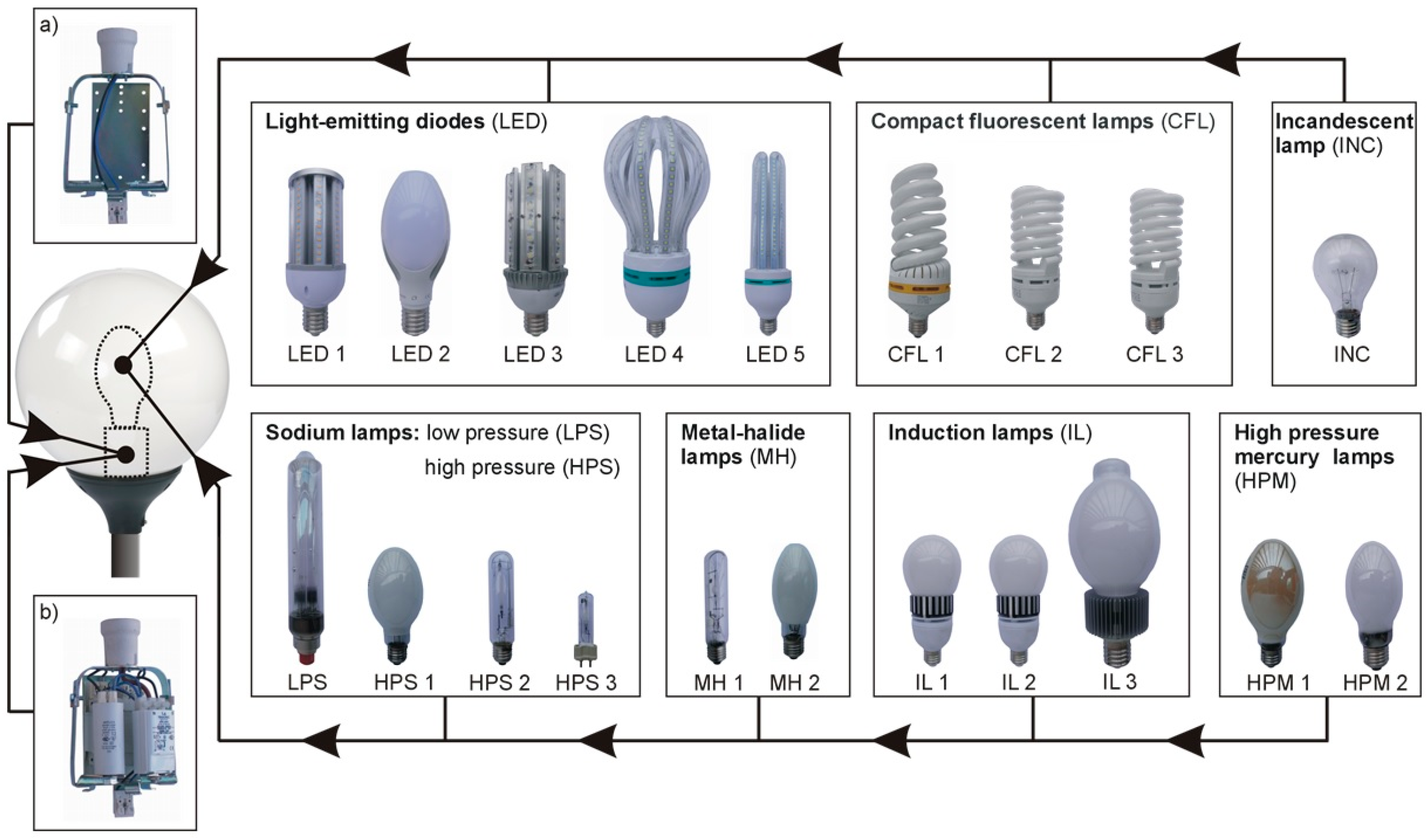
The 20 light sources were analyzed during the studies. They were five LED sources, three integrated CFL lamps, one INC lamp, one LPS lamp, three HPS lamps, two MH lamps, three IL lamps, and two HPM lamps. The distinctive light sources differ from each other by a shape of luminous body and a color of emitted light. They were placed in an opal sphere type luminaire one by one. The light sources tested together with the view of the luminaire considered and the dedicated electrical equipment are presented jointly in
Figure 2. In the case of LED, CFL, INC, and IL lamps, which are equipped with electronic power supply integrated with the lamp, the light sources were directly connected to the mains using specially designed fittings (
Figure 2a). However, in the case of HPS, LPS, IL, HPM, and MH lamps, the fittings from
Figure 2b were used. Additionally, supplying the LPS lamp was realized using the electronic supply system dedicated by the manufacturer, while the HPM lamps were supplied using a suitable choke with a capacitor.
As seen in
Figure 2, the light sources differ considerably in terms of shape, construction, dimensions, etc. From this reason, the shape of the luminous body of individual lamps will also be different. For example, in the case of INC lamps, the surface is described on a twisted pair (cylinder), and in the case of HPS2, MPS3, or MH1, the luminous body is a fragment of the toroidal surface stretched between the electrodes of light source. In turn for the lamps HPS1, MH2, IL1, Il2, IL3) the luminous body is a surface of the bulb. When we consider lamps CFL1, CFL2, and CFL3, the luminous body is the surface of the discharge tubes. However, in the case of LED sources, the luminous body is created by a set of elementary LEDs. Usually, a set of LED matrices is placed on a flat surface and individual matrices are placed at different angles (LED1, LED2, LED3, LED5). However elementary LEDs, within a single matrix, do not necessarily have to be geometrically oriented the same, as exemplified by the construction LED4. The corollary of this is the light distribution by the light source (lamp). However, the final shape of the photometric body is determined by the optical elements of the luminaire. In the case of an opal sphere type luminaire, the main element is an opal diffuser. Hence, the shape of the light sources was omitted in favor of the curves of luminous intensity in a polar coordinate system and the spatial distribution of luminous flux emitted by the luminaire (discussed in detail in
Section 3).
The spatial distribution of luminous flux emitted by the luminaire, after installing inside it an individual light source, was determined using the commonly known goniophotometric method [
34]. The measurements were carried out in the C- γ system, which is the most popular form of orientation of the space around the luminaire [
35]. In this system, the half-planes are marked with a capital letter “C” together with a digit defining the dihedral angle between the half-plane considered to be the initial and the current half-plane. However, the position of the vector on a given half-plane determines the plane angle γ related to the optical axis. Thus, any vector of luminous intensity found in the space is determined by the parameters C and γ. The measurements were supplemented by the registration of the spectral distribution of radiation emitted by the luminaire in which a specific type of light source was installed.
The authors are aware that not all types of lamps are used in practical outdoor lighting installations with opal sphere type luminaire, but from the point of view of spectral characteristics of the emitted radiation, they seem to be interesting. These lamps are undoubtedly the LPS lamps or IL lamps. The former, despite the fact that they are characterized by a very high luminous efficacy, due to practically monochromatic radiation (no possibility of color rendering of illuminated objects), their range of applications is usually limited to highways. It is worth emphasizing, however, that the point of view of an undesirable phenomenon that is light pollution, the light emitted by these lamps is very attractive (they do not disturb astronomical observations). IL lamps are also unpopular light sources, which belong to the latest generation of electric light sources of the late 20th century. Despite their extremely high durability, their relatively high price limits the range of application to the places where access to the light source is difficult (for example, due to limited accessibility to the place of luminaire installation) [
5,
6,
11,
19,
27].
In
Table 1, the fundamental data concerning the light sources tested are presented. The table includes the nominal power (P
LS), type of lamp base, and color of the light emitted.
The manufacturers, when specifying the color of the light emitted by the light source, usually operate with the parameter of the closest color temperature (CCT) expressed in Kelvin. However, in some cases, the color of light is presented in a descriptive way. The manufacturers use the following terms: warm white, white, cool white, and daylight. These terms can be found mainly in relation to the LED sources. In turn in the case of MH lamps the color of light emitted by these lamps is often expressed in the letter symbol: warm day light (WDL), white day light (BDL), neutral day light (NDL), or day light (DL). The values of the CCT and the corresponding colors of the light sources are presented in
Table 2. The data provided have were developed on the basis of the available datasheets presented by various light source manufacturers.
From
Table 2, it may be stated that the descriptive method of presentation of the color of light is not unequivocal because one can find two light sources with the same CCT (e.g., 4000 K) for which light color can be defined as white or cool white (depending on the manufacturer). As a reminder, the light color is not given in the case of INC lamps hence the item “x” is placed at position No. 9 in
Table 1. The color of the light emitted by INC lamps depends on the working temperature of the tungsten wire (which depends on the rated power of the lamp) and ranges from about 2400 K to about 2900 K.
On the basis of the data obtained from the laboratory measurements, the simulations of the light intensity distribution were carried out using DIALux software. First, the files with photometric data of the luminaire (LDT type files) were generated considering all 20 light sources installed in the luminaire. Secondly, a virtual ground model of a square shape was created with location in its central position the lantern with the same luminaire as the luminaire tested in laboratory experiment. The grass ground was simulated. and the spectral reflectance of the grass was defined. Two typical ways of installation of the light sources in the luminaire were analyzed in simulations: with the handle down and the handle up. After receiving the light intensity distribution for the distinctive cases from the simulations, the calculations were made to assess the light pollution effect considering the total luminous flux emitted by the luminaire, the shape of the photometric body, and the spectral reflectance of the ground.
3. The Results of the Laboratory Measurements
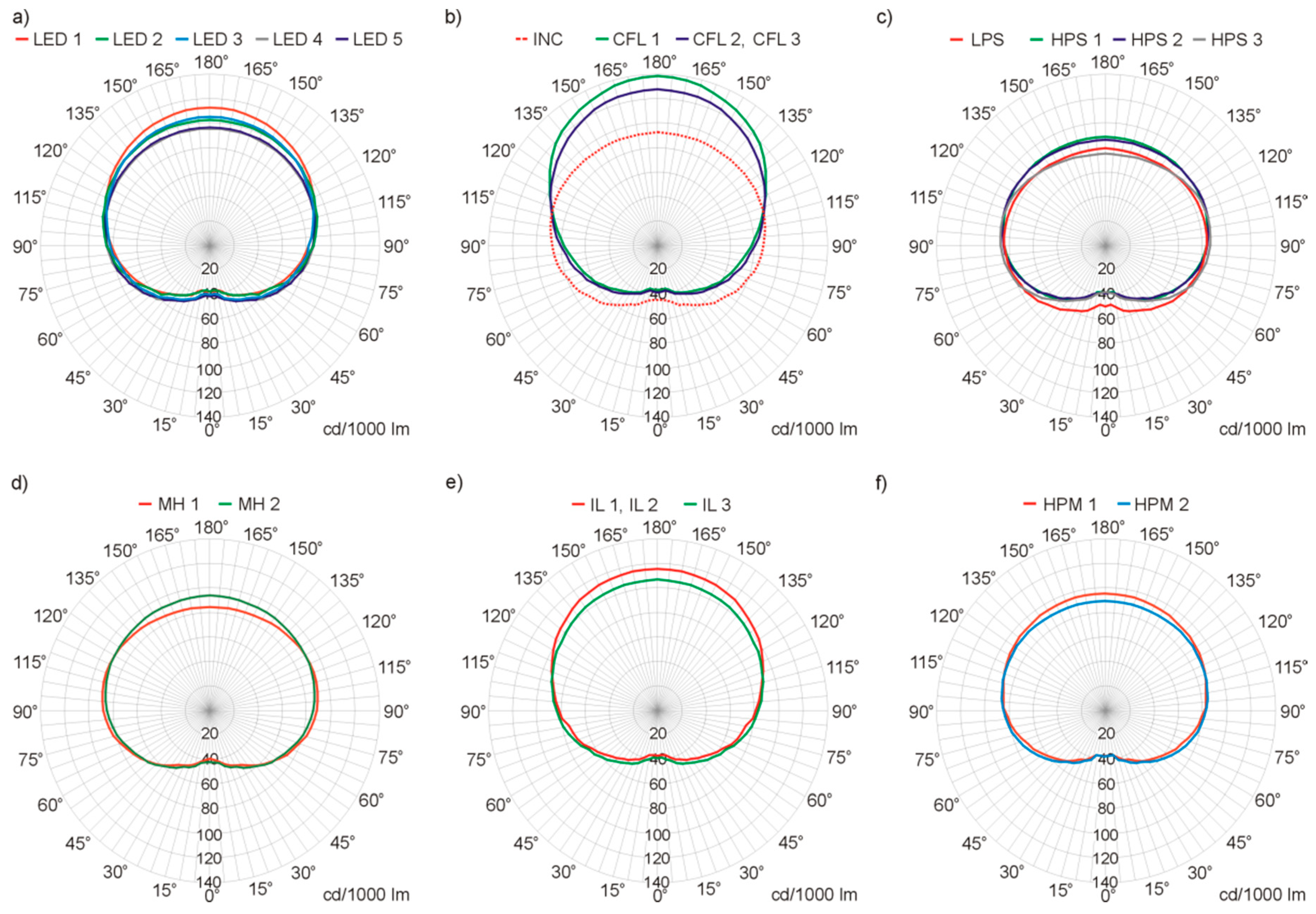
The basic method of presenting the distribution of light by the luminaire is the photometric solid [
10,
21,
36]. It is a set of spatially distributed vectors of luminous intensity originating in the light center of the luminaire. In view of the fact that in each case of the light sources installed in the luminaire the photometric body represents the symmetrically rotational form, the data from the measurements were presented as the flat graphs in the polar coordinate system as in
Figure 3. This form of data presentation seems to be more readable and does not pose any difficulty in imagining the shape of the photometric solid. The results are presented in cd/1000 lm, referring to the values of luminous intensity to the light source with the reference luminous flux of 1000 lm.
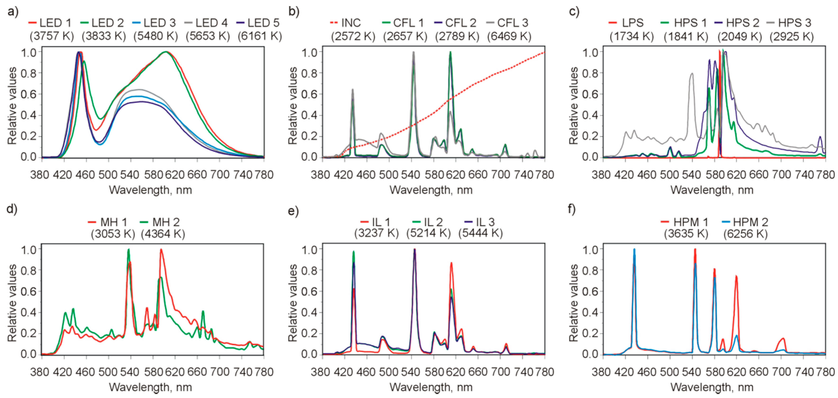
Figure 4 presents obtained spectral characteristics of radiation emitted by the opal sphere type luminaire considered for the distinctive light sources installed inside it. The values given in brackets (in the legend) are the CCFs of the light emitted by the luminaire.
On the basis of the measurements carried out, the selected parameters of the opal sphere type luminaire were determined, taking into account the type of the light source used. The values of these parameters are summarized in
Table 3.
One of the basic parameters of the luminaires is a rated luminous flux
Φn that is the total luminous flux sent by the luminaire operating at nominal conditions. If a horizontal plane is carry through the opal sphere type luminaire (in
Figure 3 it will be a horizontal line passing through the center of the graph), the total luminous flux of the luminaire
Φn will be divided into an upward flux
ΦΛ and a lower downward flux
ΦV. In
Table 3, both components of the luminous flux (
ΦΛ and
ΦV) are given in a percentage scale, taking as a reference point the total luminous flux
Φn emitted by the luminaire with a specific light source installed inside it. Thus, the total luminous flux
Φn is a sum of both components (
ΦΛ and
ΦV). These components were calculated on the basis of distribution of light emitted by the luminaire, presented graphically in
Figure 3. From the point of view of the light pollution problem, it is not advisable to emit a luminous flux created directly by the luminaire (i.e., it is advisable that
ΦΛ = 0). Unfortunately, in the case of opal sphere type luminaire (depending on the light source installed inside it),
ΦΛ is in the range from 53% to 65%. It means that more than a half of the total luminous flux is sent in the direction of upper half-space. Obviously, this is in the case when the luminaire of opal sphere type is installed with the handle down (as situations 1a, 1b, 1c, 1e from
Figure 1). The situation looks a little bit more optimistic when the luminaire is positioned with the handle up (situation 1d from
Figure 1). In this case,
ΦΛ is in the range from 35% to 47%. It means that less than a half of the total luminous flux is sent in the direction of the upper half space. Unfortunately, in practical solutions, where economic considerations play an important role, the luminaire is typically installed directly on the top of the pole (
Figure 1e). This solution avoids the additional costs related to the need to install arms or to use the more expensive support structures enabling the luminaire to be mounted with the handle up.
The next parameter of the luminaire is the nominal active power Pn. It is the sum of the power consumed by the light source and the power consumed by the components of electrical equipment of the luminaire if present (e.g., electronic supply system of the lamp). In the case of light sources that are designed to be supplied directly from the 230 V mains, the active power of the luminaire is determined solely by the installed light source. It is therefore important to notice that, by considering only the declared power of the luminaire, the final conclusions may be wrong.
The parameter considered for the luminaires is also luminous flux
Φn. A good example illustrating the problem of analysis of luminous flux is comparison of the lamps IL1 and IL2 (positions 16 and 17 in
Table 3). In the case of both lamps, the power consumed by the luminaire is identical (P
n = 31 W) whereas the luminous flux differs by approximately 8.5%. Therefore, if induction lamps are chosen, it will be more beneficial to install the IL2 source than IL1 in the luminaire.
The luminous flux
Φn and the active power P
n may be assessed jointly through a parameter called luminous efficacy η
n. It is a key parameter in the context of energy efficiency. The higher the value of η
n, the more energy efficient the luminaire. The luminous efficacy is designated as the quotient of the total luminous flux
Φn sent by the luminaire and the active power P
n taken by the luminaire from the mains. Taking into account the above description as well as the data included in
Table 3, it may be stated that the most advantageous solution in terms of energy efficiency (η
n = 97 lm/W) is equipping the luminaire with LPS. However, the smallest luminous efficacy of the luminaire (η
n = 12 lm/W) was obtained for the INC lamp as the light source. This fact and the very low durability of the incandescent lamps (average lifetime equal to 1000 h) explain why these light sources have been superseded in the lighting of outdoor areas.
Considering the color of emitted light, it is important to remember that the color is defined using the above-mentioned CCT parameter. The lower the CCT value, the warmer the color of the emitted light. The warmest color among the used light sources was associated with LPS (1734 K), and the coldest color concerned CFL 3 (6469 K). The use of luminaires equipped with light sources of low color temperature is therefore recommended. In general, it is clear that, regarding lower color temperature, within the spectral distribution of radiation there is a smaller amount of short-wave radiation, and this short-wave radiation is more strongly dispersed in the atmosphere (on oxygen and nitrogen molecules) than the longer radiation waves. For this reason, the International Dark-Sky Association (IDA) recommends the use of luminaires of a CCT not exceeding 3000 K [
37]. In turn, in the context of minimizing the electricity consumption for lighting purposes, it is preferable to use the luminaires with the light sources of a high CCT.
In the case of outdoor lighting, due to low levels of luminance, the eye is adapted to twilight (mesopic) vision. In twilight vision conditions, the curve of the eye’s luminous efficacy is shifted toward short-wave radiation, and its absolute value is increased. This fact has practical and economic meaning because in the case of the luminaires in which the radiation spectrum consists of a large component of the radiation in the short-wave range, the actual effect assessed by outdoor lighting users will be greater than it was calculated [
34,
38,
39].
CCT does not contain information about the appearance of illuminated colors of illuminated objects. A parameter that is a measure of the quality of color rendering under the light emitted by the luminaire is the color rendering index (CRI). Its maximum value is equal to 100. It is considered that the higher the value of this indicator, the better (faithfully) the colors of illuminated objects are rendered. Excluding LPS, for which CRI is not determined due to the almost monochromatic nature of the radiation, the lowest CRI value was obtained for HPS1 (CRI = 19) and the highest CRI was associated with the INC lamp (CRI = 98). When choosing a light source, high CRI lamps are not used very often for outdoor lighting due to economical reasons. The issue concerning the required CRI value, excluding outdoor workplaces as per CIE S 015/E: 2005 [
20], is not included in the standards. However, it is important to point out that installing the light sources characterized by low CRI may result in the unnatural look of illuminated objects. This takes place especially in the case of sodium lamps (of low CRI), which may change or distort the colors of plants or people’s faces. In the case of green areas, it is assumed that the overall color rendering index should not be less than 60.
4. Simulation Results and Their Analysis
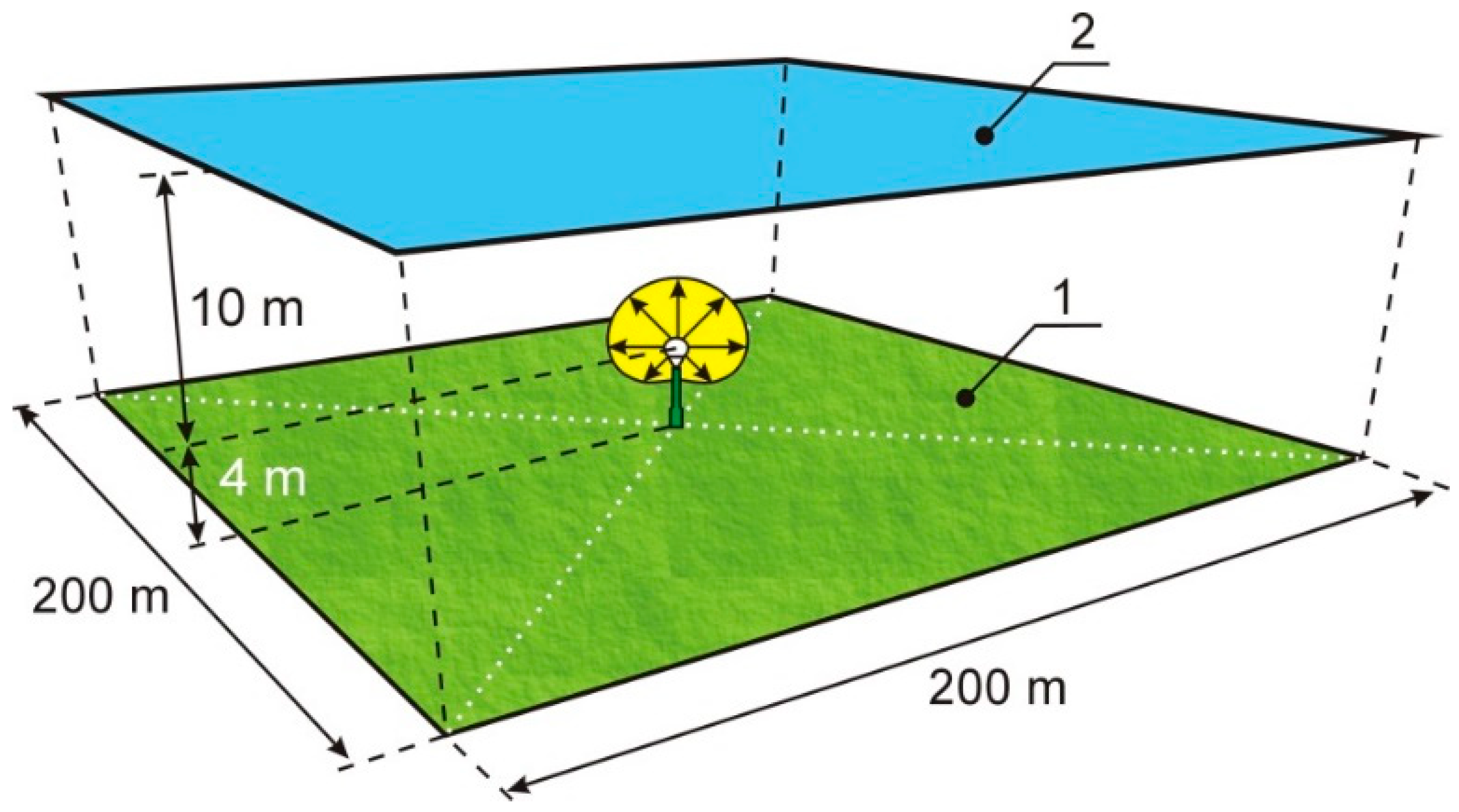
As was mentioned above, the LDT type files with photometric data of the luminaire were generated for 20 cases of light sources installed in the luminaire. After generation of the files, a virtual ground model was created, which was shaped in a square with dimension 200 × 200 m. In its central position, a lantern equipped with opal sphere type luminaire was placed. The luminaire was installed at a height of 4 m, which is a typical height for the installation of the luminaires in parks, squares or avenues with footpaths. At a height of 14 m (10 m above the place of installation of the luminaire as recommended in reference [
18]) and in parallel to the ground a calculation grid was placed, as shown in
Figure 5. The grid includes 40,401 evenly distributed calculation points. The distance between the points was 1 m. The size of the calculation grid was chosen in such a way that the calculated values of illuminance in points placed on the edge of the grid assumed zero or near zero values (0.01 lx).
Due to the large side length of the ground (200 m) in relation to the height of the luminaire installation (4 m), the lantern in
Figure 5 was enlarged for better explanation of the approach for calculation. It is worth noting that, from the point of view of light pollution, the reflective properties of the ground are also important in the analysis. Part of the luminous flux emitted by the luminaire goes to the ground, where it is reflected and directed upward toward the calculation grid. Thus, the reflecting surface of the ground should be treated as a secondary light source. A parameter describing the properties of a given surface is total reflectivity. It is given in the form of a decimal fraction or as a percentage value. In the calculations, it was assumed that the lantern with opal sphere type luminaire is located on a ground with a total reflectivity of 16%, which is typical value for the ground covered with grass.
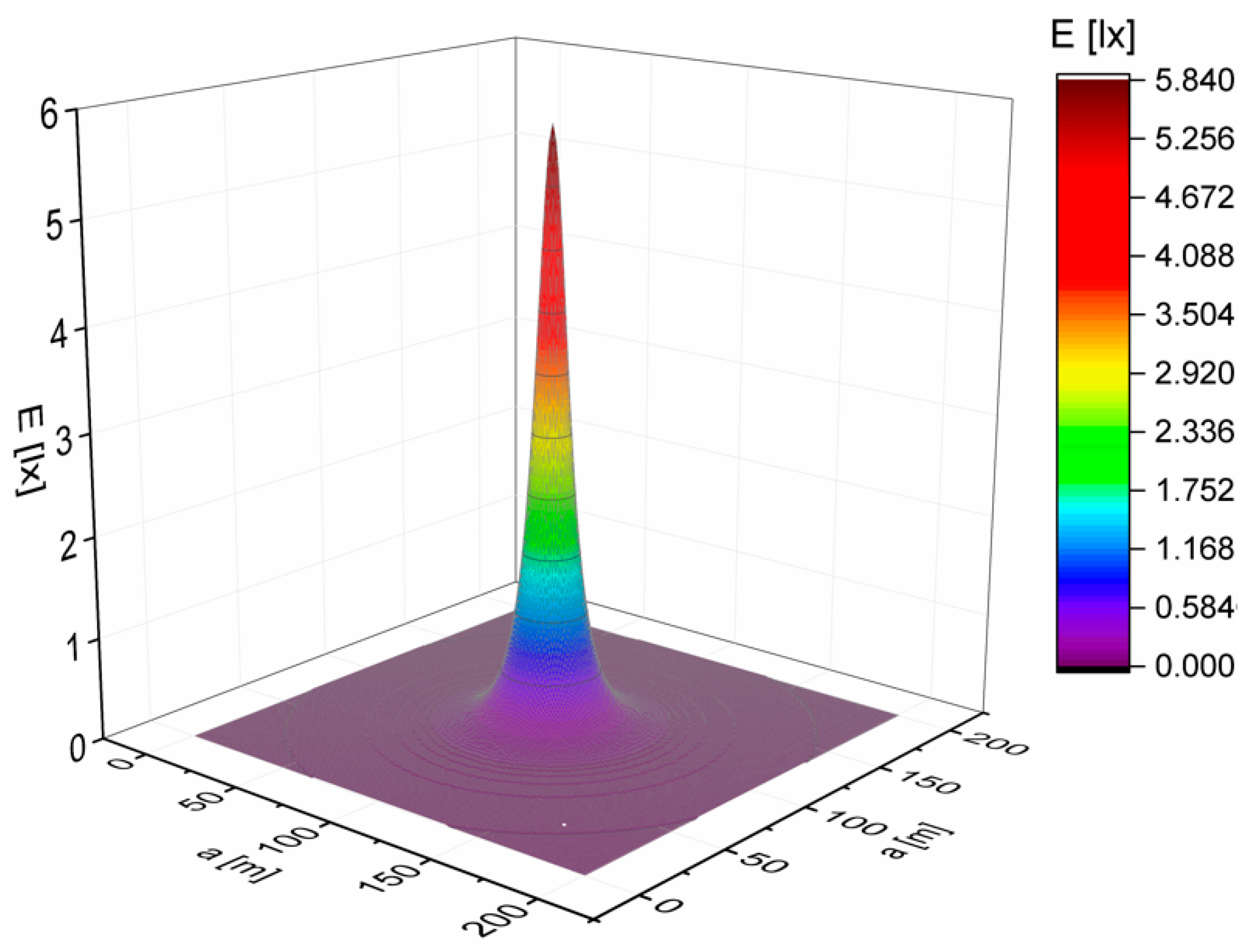
Due to the large number of variants considered (20 light sources installed in the opal sphere type luminaire and two positions of mounting the light sources), the presentation of the distribution of illuminance was limited to one case—the luminaire with the HPS2 lamp installed. Based on data obtained from the DIALux software the visualization was prepared, illustrating the distribution of illuminance (
Figure 6). The results presented refer to the total illuminance E [lx], taking into account both components of the luminous flux of the luminaire (
ΦΛ and
ΦV).
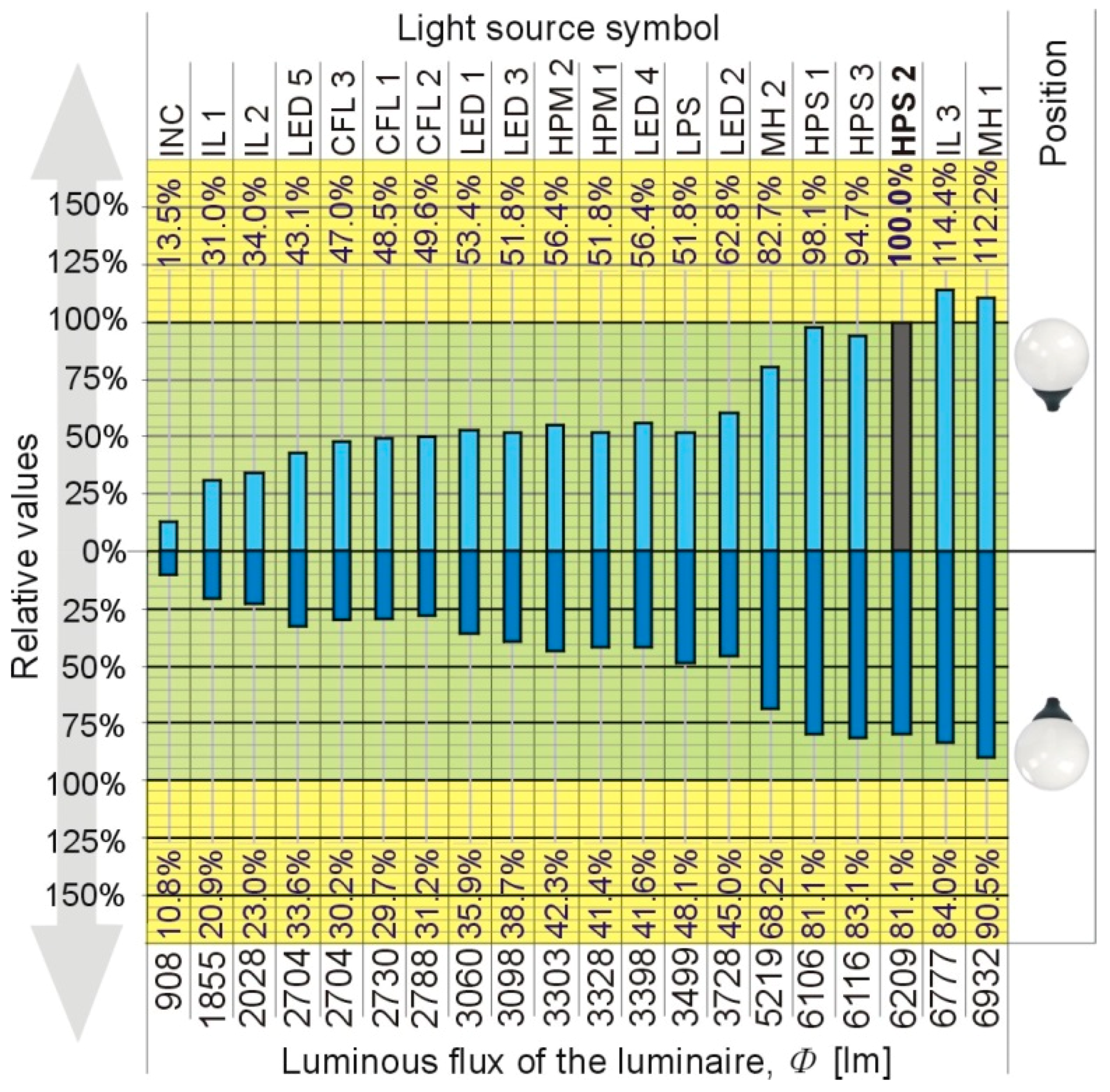
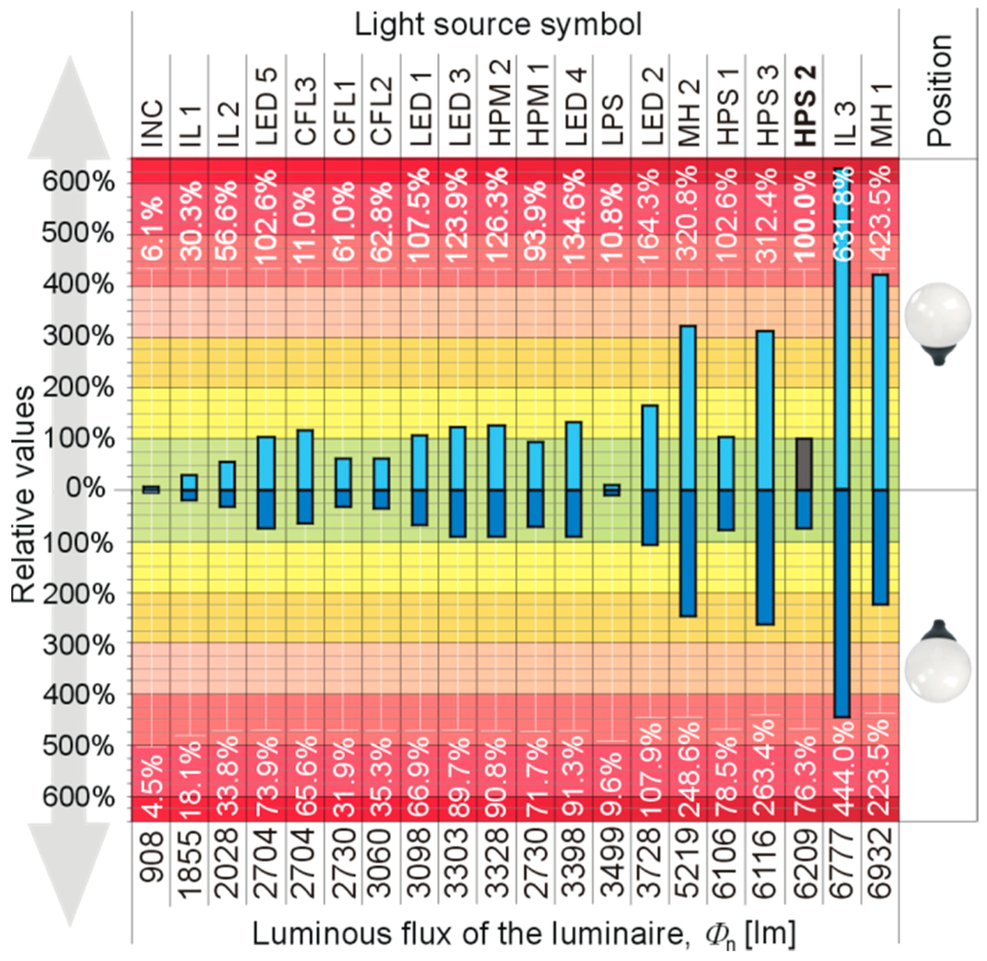
Given the size of the surface of the computational grid (a x a) and the distribution of illuminance on its surface, one can calculate the luminous flux that reaches it. The calculations were carried out for each of the 20 light sources installed in the luminaire, including two positions of the luminaire. The results of the calculations in graphical form are shown in
Figure 7. The values of the luminous flux emitted are presented in percentages, taking as the reference the luminous flux emitted by the lantern with the luminaire handle down and cooperating with the HPS2 lamp (symbol HPS2 is marked by bold font in
Figure 7). It is worth noting that HPS2 lamps are still a very popular light source in outdoor lighting, and the opal sphere type luminaires are usually mounted with a handle down. The calculation results shown in
Figure 7 take into account two components of the luminous flux—sent directly by the luminaire and reflected from the ground.
The results of the calculations in
Figure 7 were arranged taking as a criterion the total luminous flux emitted by the luminaire (from the lowest value to the highest). Based on the data obtained in this field, it can be noted that, in the case of some light sources, the increase in luminous flux does not cause an increase of the effect of light pollution. The reason for this is the difference in the way the light is distributed by the luminaire (as illustrated in
Figure 3). Thus, the effect of light pollution is influenced by both the value of the total luminous flux of the luminaire and the shape of the photometric body, which changes itself with the change of the light source.
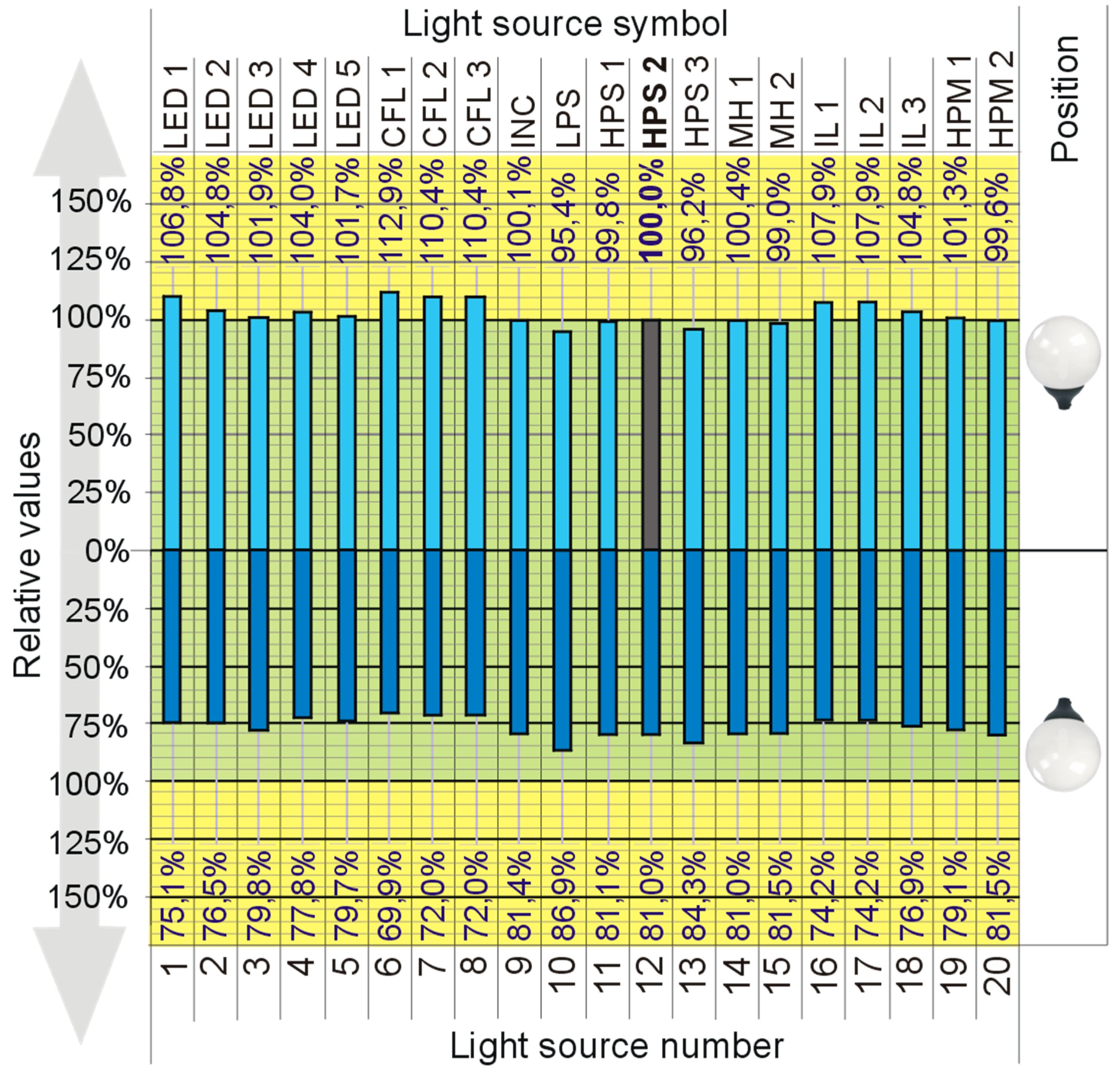
Assessing the influence of the shape of the photometric body on the light pollution effect the calculations were carried out again in the DIALux software. In these calculations, it was assumed that the total luminous flux emitted by the luminaire (regardless of the type of light source installed inside it) is identical and is the same as in the case of mounting the HPS2 lamp (that is 6209 lm). The results of calculations made are shown in
Figure 8. As before, the values were normalized to the lantern with the luminaire with handle down cooperating with the HPS2 lamp. Analyzing the data from
Figure 8, it can be seen that replacing the HPS2 lamp with another light source (as a result of changing the shape of the photometric body) may influence the effect of light pollution. The least optimistic results from the point of view of light pollution were observed for CFL1 and CFL2. In the case of luminaire handle down, replacing HPS2 with CFL1 may contribute to a 10.4% increase in light pollution, whereas in the case of a CFL2, this increase is equal to 12.9%.
The results of the calculations presented in
Figure 7 and
Figure 8, due to the specificity of the DIALux software, do not take into account the spectral distribution of the light emitted by the luminaire. The DIALux does not take into account the spectral characteristics of light sources but only considers their luminous flux and the way of its distribution. The situation is similar in the case of illuminated surfaces whose reflective properties are characterized by the total reflectivity. In practice, this means that all spectral characteristics characterizing either the light sources or illuminated surfaces are treated by the software as linear (in the entire visible range). In order to take into account the interaction of light of a given spectral distribution (
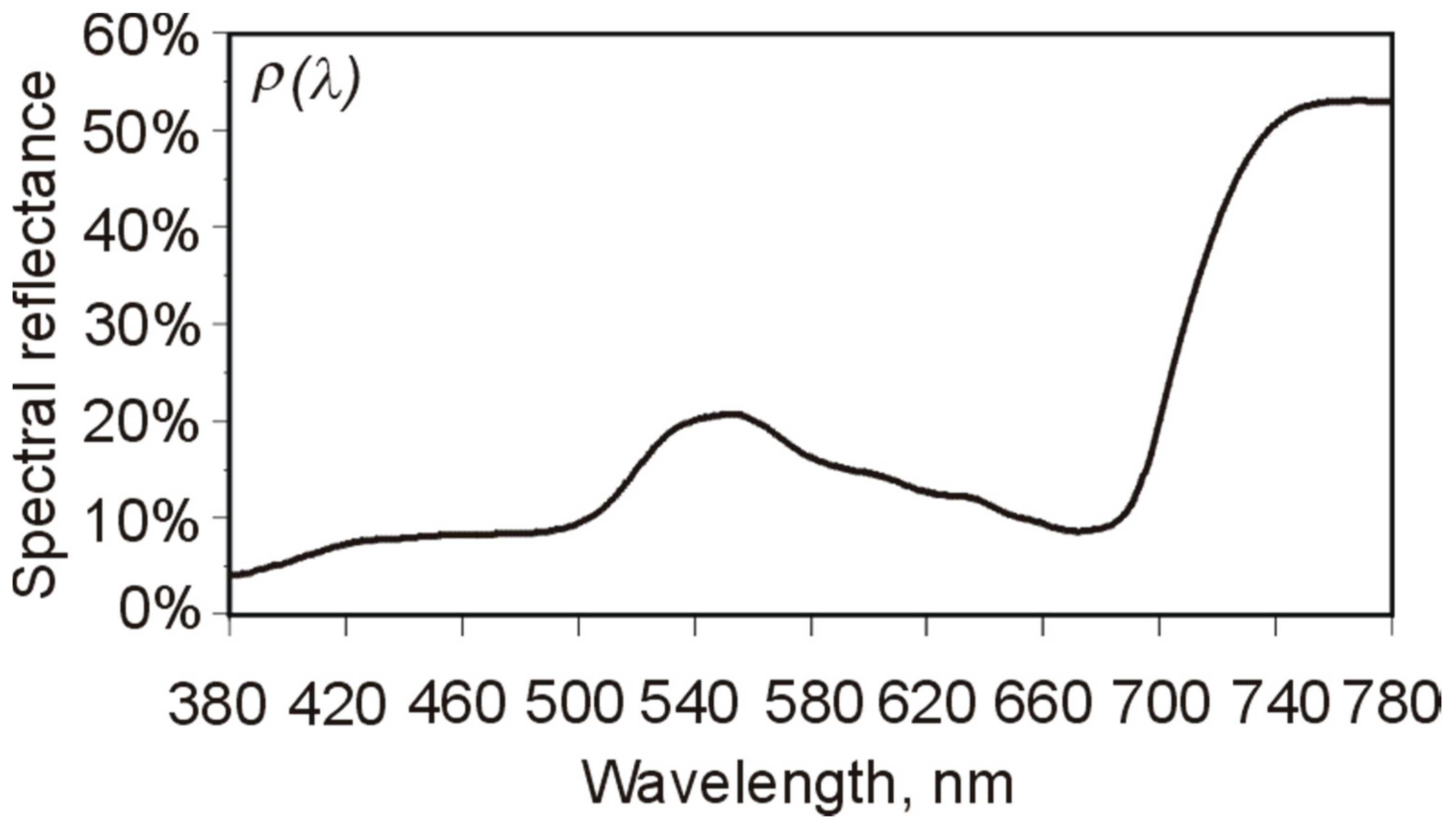
Figure 4) with reflective properties of the illuminated ground, it is necessary to take into account the fact that in practice the surfaces possess selectivity of reflection. This means that the value of reflectance (in relation to the ground) is determined by the wavelength λ.
A parameter characterizing the selectivity of the reflection is a spectral reflectance (λ).
Figure 9 presents the spectral reflectance (λ) of the grass. The data necessary to plot this spectral reflectance was taken from the Jet Propulsion Laboratory (JPL) spectral library, which is available on the National Aeronautics and Space Administration (NASA) website [
40].
Knowing the spectral reflectance of the ground and the spectral distribution of radiation emitted by the luminaire (
Figure 4), it is possible to determine the spectral characteristics of radiation reflected from the ground. This part of the calculations, taking into account the effect of the spectral distribution of light emitted by the luminaire together with the spectral reflection properties of the ground, was carried out outside the DIALux software using the original authors’ tool. This tool allowed for the implementation of the results from the DIALux software and introduced the rest of the data, such as the distribution of the spectral radiation emitted by the luminaire and the reflective properties of the ground (in the form of spectral reflectance).
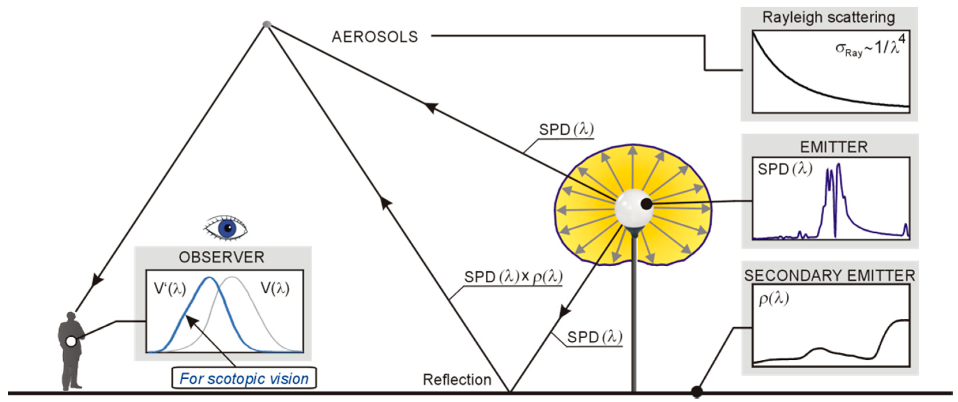
One of the consequences of emitting radiation into the sky by electric lighting is the increase of brightness of the night sky. Numerous mathematical models are used to quantify the brightness of the night sky however most of them are very complicated. In general, the Rayleigh scattering phenomenon is taken into account in the methods of modeling the night sky pollution. The formed relationship between the wavelength and the intensity of its dissipation says that the intensity of the scattered light is inversely proportional to the fourth power of the wavelength (
σRay ~
λ−4). The light is scattered on particles much smaller than the length of the scattered wave. In the case of larger particles (i.e., the size of which is larger than the wavelength), there is Mie scattering, which is inversely proportional to the wavelength (
σMie ~
λ−1). In the case of Mie scattering, light is scattered in small angles compared to the initial course of rays, so that this phenomenon does not have such a strong effect on light pollution as Rayleigh scattering [
31].
In the process of assessing the pollution of the night sky, an observer can also be considered. If we assume that the observer of the night sky will be a human, then when quantifying the radiation reaching him/her, the spectral sensitivity of the human eye should be taken into account. International Lighting Commission (CIE) adopted unified values of the relative spectral luminous efficacy: in the daytime vision (photopic) V(λ) and in the night vision (scotopic) V′(λ). There is also a mesopic vision, which was further specified in [
41]. In this document, a mathematical dependence was given to determine the curve of the eye’s sensitivity V
mes(λ). The choice of the appropriate eye sensitivity curve depends on the luminance level. It is assumed that the V(λ) curve applies to the luminance L ≥ 5 cd/m
2, while for small levels of luminance L ≤ 0.005 cd/m
2, the eye is adapted for night vision, and the curve V′(λ) applies. The values from the range (0.005–5) cd/m
2 correspond to twilight vision represented by V
mes(λ). The issue of the clarity of the night sky is a complex issue and goes beyond the scope of this paper. However, when analyzing the works which present the measured values of the brightness of the night sky [
24], it can be stated that luminance in summertime usually does not exceed 0.005 cd/m
2. Thus, in further considerations, the curve V′(λ) is considered when assessing the light pollution of the night sky. Both the V′(λ) and scattering were considered in authors’ software of Rayleigh. An illustration of the factors taken into account when assessing the pollution of the night sky is shown in
Figure 10.
The results of the calculations, which take into account the shape of the photometric solid (
Figure 3), spectral distribution of radiation emitted by the luminaire (
Figure 4), spectral reflectance (
Figure 9), Rayleigh scattering, and spectral sensitivity of the human eye V′(λ), are shown in
Figure 11. Individual values have been normalized to the luminaire with the HPS2 lamp installed with the handle down. The results shown relate to luminaire of which luminous flux differs as in
Table 3.
They are presented on the x-axis with reference to particular lamps and assuming, as a criterion, the value of the luminous flux emitted by the luminaire (from the lowest to the highest) with the different type of light sources installed inside the luminaire. In addition, the data in this figure concern both considered methods of installation of opal sphere type luminaire. This form of data presentation (according to the authors approach) will allow us to analyze how the considered factors affect the light pollution effect. For several light sources (INC, IL1, IL3, CFL1, CFL2, HPM1, LPS), the values obtained are below 100%, which is a desirable phenomenon from the point of view of light pollution effect. In the case of other lamps, the values exceed 100%, which means that replacing the classic HPS2 lamp with these light sources will be associated with an increased light pollution effect.
The special attention should be put on the cases of HPS1 and HPS3. Although the luminous flux of the luminaire in these cases differs slightly (about 0.16%), due to the different spectral characteristics of the radiation, the degree of light pollution generated (when the luminaire is installed with handle down) will be greater more than three times in the case of HPS3 in comparison to the HPS1. This means that the important factor affecting light pollution is not only the value of the luminous flux emitted in the upward space but the spectral characteristics of the emitted radiation.
In practical conditions, the replacement of a light source in a luminaire involves a change in the luminous flux. The different values of the luminous flux of a luminaire fitted with a given light source make it difficult to analyze the influence of the light source used on the light pollution effect. In other words, it is difficult to assess how the spectral distribution of radiation emitted by the luminaire affects the light pollution. Therefore, it would seem to be appropriate to use in the luminaires such light sources, in which the luminous flux emitted by the luminaire will be identical. In practice, meeting this requirement is rather difficult to perform. From this reason the conclusions presented below assume that regardless of the type of the light source installed in the luminaire the luminous flux is the same (
Figure 10). The distinctive results of the calculations have been again normalized to the luminous flux emitted by the luminaire equipped with a HPS2 lamp. In other words (as before), it was assumed that regardless of the type of light source used in the luminaire, the total luminous flux of opal sphere type of luminaire will be equal to 6209 lm. With regard to all lamps, the calculations were repeated, and their results were placed (as before) in the form of a bar graph in
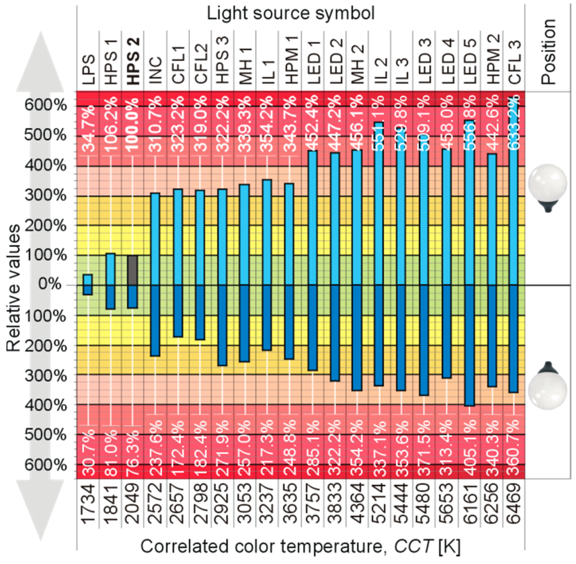
Figure 12. This time, the light sources were arranged by accepting as a criterion the value of CCT. This form of data presentation allows us to analyze the influence of the color of light emitted (described by the CCT parameter) on light pollution.
Analyzing the data presented in
Figure 12, it can be seen how important the role of the spectral distribution of radiation emitted by the luminaire is for the effect of light pollution. Despite the same value of the luminous flux emitted by the luminaire, the potential impact on increasing the sky glow will be different. The least optimistic results were obtained for the CFL3 lamp (of CCT = 6469 K). Installing it in an opal sphere type luminaire as replacement of conventional HPS2 light source will cause more than six times higher impact (633.2%) on effect of light pollution. This unfavorable phenomenon can be minimized (up to 360.7%) by setting the luminaire with the handle up. As expected, the smallest impact on the light pollution effect was obtained by installing an LPS lamp in the luminaire.
In the case of the luminaires of opal sphere type, it happens that lighting modernization concerns only replacement of the light source in the luminaire. Analyzing the data presented in
Figure 11 and
Figure 12, one can analyze the consequences of this state of affairs as follows. From the end of the 20th century to the present, there has been a global interest in energy efficiency issues with an accent on environmental related issues where LED sources emitting white light play a significant role in outdoor lighting. Due to the higher content of short waves in the radiation spectrum (which usually increases with CCT), in external lighting applications (due to mesoptic vision) LED sources with higher color temperatures are preferred. Unfortunately, strong short-wave scattering intensifies the effect of light pollution. Installing the LED sources considered herein as replacements of HPS2 lamp typically applied in opal sphere type luminaire is undoubtedly a favorable solution from the point of view of energy efficiency, but it will adversely affect light pollution. Depending of the type of LED sources, an increase of light pollution takes place. In the case of the luminaire with the handle up this increase reaches even 556.8% in the most unfavorable situation (LED 4 in
Figure 12). Hence, when choosing the light source of white color of light, a compromise should be found between light efficiency and impact on light pollution.
Due to the date of purchase of LED sources for the studies the markings such as white, cool white or daylight (as in
Table 2) were widely used by the manufacturers. As the LED sources have been developed dynamically, improved or new constructions have been proposed that have not been used so far. Currently, manufacturers and distributors have LED sources with a warm white color (e.g., 2700 K) and luminous efficacy exceeding 100 lm/W. There are also LED sources with even lower color temperatures (e.g., 2500 K, 2200 K, and even 1800 K—i.e., similar in value to LPS) and luminous efficacy close to or equal to 100 lm/W. The use of this type of light source will undoubtedly cause a reduction of light pollution. However taking into account the high price of such the light source (the cost of the lamp is several times higher than the price of the opal sphere type luminaire), the luminous efficiency of the luminaire (
Table 3), which is lower not only for LED lamps but also for HPS lamps, and additionally, according to the data given in
Figure 12, it is rather difficult to consider an argument for installing this type of light source in the luminaire.


