Abstract
This paper presents a finite control-set model predictive control (FCS-MPC) based technique to reduce the switching loss and frequency of the on-grid PV inverter by incorporating a switching frequency term in the cost function of the model predictive control (MPC). In the proposed MPC, the control objectives (current and switching frequency) select an optimal switching state for the inverter by minimizing a predefined cost function. The two control objectives are combined with a weighting factor. A trade-off between the switching frequency (average) and total harmonic distortion (THD) of the current was utilized to determine the value of the weighting factor. The switching, conduction, and harmonic losses were determined at the selected value of the weighting factor for both the proposed and conventional FCS-MPC and compared. The system was simulated in MATLAB/Simulink, and a small-scale hardware prototype was built to realize the system and verify the proposal. Considering only 0.25% more current THD, the switching frequency and loss per phase were reduced by 20.62% and 19.78%, respectively. The instantaneous overall power loss was also reduced by 2% due to the addition of a switching frequency term in the cost function which ensures a satisfactory empirical result for an on-grid PV inverter.
1. Introduction
In an on-grid photovoltaic (PV) system, the inverter is considered the most vital component of the system. An apposite inverter controlling is necessary for achieving moderate power loss, total harmonic distortion (THD), and the safety and reliability of the grid [1,2]. Various types of control mechanisms, including linear (proportional–integral (PI) [3,4], proportional–resonant (PR) [5], repetitive [6], deadbeat control [7], etc.) and nonlinear techniques (sliding mode control (SMC) [8], space vector modulation (SVM) [9,10,11], predictive [12,13], etc.) are available in the literature. Various control variables, such as current, voltage, real, and reactive power, are considered in the abovementioned controllers. Over the other controllers, the current controller provides a higher input/output response time, easiness to mitigate the harmonic component using an active filter, inherent over-current protection, and easier control to inject power into the system. Therefore, a current-based control technique was mainly considered in this research work. The advantages and disadvantages of the various current based controls are shown in Table 1.

Table 1.
Comparison of the different current controllers [5,19,20].
It can be seen that predictive controllers overcame the tracking accuracy, transient response, and higher THD problems of the other controllers and became popular due to the fact of their eye-catching advantages. Predictive controllers underwent several developments over the years and are classified into several categories as shown in Figure 1 [14,15]. Among these control strategies, model predictive control (MPC) is treated as a favorable strategy because of its quick response, lucidity, nonlinearity, and capacity to handle numerous systems constraints [16,17,18].
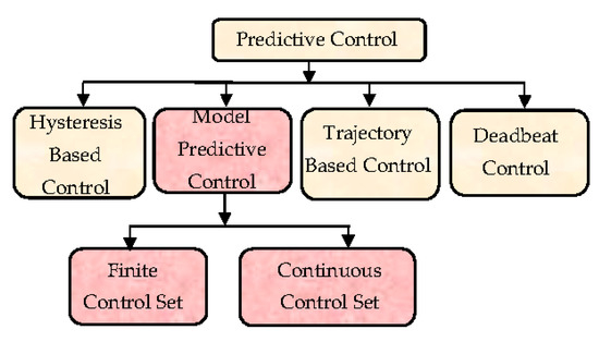
Figure 1.
Classification of the predictive control technique.
The MPC can be partitioned into two subsets: a continuous control set (CCS) and a finite control set (FCS) MPC [21]. In CCS MPC, a pulse width modulation (PWM)-based modulator is utilized to transmit the output from the controller [22]. The modulator provides the switching signal to the converter. Hence, the achievable reference esteems exchanged to the modulator must be determined and a cost function is utilized to select the most appropriate reference set. However, FCS-MPC can generate the switching signals for the converter without a modulator [23,24]. The optimization can be improved to the expectation level, as the switching states are finite in number and can be used to assess a cost function. The state with the least cost is chosen and applied to the converter. Therefore, this FCS-MPC technique is utilized in the research work.
Recently, MPC is widely used for the on-grid PV inverter. For critically controlling the dc voltage of an on-grid PV inverter, a predictive control strategy was proposed in Reference [25] based on the relationship of the energy balance during the control period. For ameliorating the on-grid PV current, the exact transient analytic model was proposed in Reference [26]. For an on-grid inverter utilizing a PV source, a model predictive direct power control technique was designed in Reference [27] which can efficiently track the insolation change and the output power with an improved steady-state and dynamic response. Based on the mathematical model of the three-phase on-grid inverter, a predictive current control technique in a static α–β frame was presented in Reference [28]. It was shown that the controller can easily track the change of the maximum power point of the PV and penetrate active power to the grid with low distortion. To improve the stability of the power system, an MPC-based low voltage ride-through method was proposed in Reference [29] for the on-grid PV inverter, where a detailed analysis of the power imbalance problem during the symmetrical grid voltage drop was presented. The use of an LCL filter in the output of the on-grid inverter creates new resonance due to the grid impedance variation. For damping these resonances, extra passive component or an extra loop may be added to the controller which also adds complexity to the system. To solve this problem, an MPC-based controller was proposed in Reference [30] without having extra sensors against the variation of the grid impedance and LCL filter parameters. Again, due to the low number of switching states in a single-phase on-grid inverter, a high-quality MPC-based controller was proposed in Reference [31] with an LCL filter to reduce the THD of the injected current to the grid. The proposed controller is robust, fast, and has an acceptable current THD with stability against the variation of the grid impedance.
The abovementioned MPC optimizes the pre-defined cost function of the system based on the system model and constraints [32,33]. Among each sampling instant, when the optimization is settled, the controller will apply just the primary component of the succession utilizing the new estimated information and obtaining another sequence of the optimal actuation each time. The control calculation required long estimation times and, therefore, high switching frequency-based applications were unrealistic before. The rapid technological advancement in the field of microprocessors shines new light on solving the computational problem of MPC. However, the high switching frequency results in a higher amount of switching loss, which is also responsible for the lower efficiency, stability, and safety of the system. The most common strategy for lowering the switching loss is by reducing the switching frequency. However, for maintaining the stability and limitable THD of the system, the switching frequency cannot be lowered too much. Therefore, a trade-off between current THD and switching frequency is always maintained. To overcome these existing problems, various strategies were proposed in the literature [34,35,36,37,38,39]. A switching strategy-based FCS-MPC technique was proposed in Reference [34] to reduce the switching loss and ensure stable operation. Again, two different predictive current-controlled methods were presented in References [35,37] to reduce the switching frequency and THD. Two different predictive power control techniques were presented in References [36,38] to reduce the switching frequency. Furthermore, a model predictive voltage control was proposed in Reference [39] to reduce the switching frequency. The mentioned strategies along the proposed methodology are compared in Table 2. It can be seen that the existing techniques only consider the switching loss of the system, but the other two-loss components (i.e., conduction and harmonic) are not considered, and they have a significant contribution to the power loss of the system. The presented research work aimed to fill this research gap.
Table 2.
Switching frequency and switching loss reduction-based techniques in predictive control.
An FCS-MPC-based two-level, three-phase, on-grid PV inverter (as shown in Figure 2) is proposed in this research work. The proposed controller simultaneously controls the inverter side current employing reference current tracking and switching frequency. The controller generates an optimal switching state for the insulated gate bpolar transistor (IGBT)-based inverter according to a predefined cost function. The cost function is designed to improve the tracking accuracy and reduce the number of switching commutations. The system parameters are initialized properly, and the simulation works along with the hardware realization of the controller being performed. In brief, the contributions of this research work are:
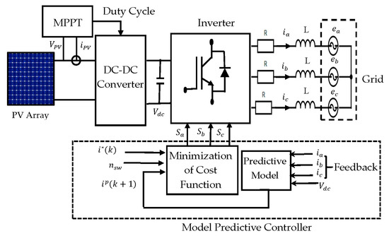
Figure 2.
Block diagram of the proposed controller-based system, where the photovoltaic (PV) array is connected with the dc/dc converter via maximum power point tracker (MPPT) to provide the requisite dc-link voltage to the on-grid inverter, and the switching signals are selected by the proposed model predictive control based controller.
- i.
- Design of an MPC-based, on-grid PV inverter for energy-efficient control;
- ii.
- Analysis of the effect of adding a switching frequency in terms of the cost function of MPC and to reduce the switching frequency of the control device with an appropriate weighting factor;
- iii.
- Calculating and analyzing the overall power loss of the proposed system and comparing it with a conventional MPC-based system.
The paper is organized into six sections. The motivation behind the research work and the contributions of it are presented in Section 1. Section 2 presents the design of the proposed controller. Section 3 presents the analysis of the power loss in the system. The simulation results and hardware deployment are delineated in Section 4. The comparison between the proposed controller and conventional FCS-MPC is presented in Section 5. Finally, the outcomes are summarized and a conclusion is drawn in Section 6.
2. Proposed MPC-Based Controller
The block diagram of the proposed controller-based, on-grid PV system is shown in Figure 2, where the PV system includes a maximum power point tracker (MPPT) [40,41], and the dc/dc converter is utilized to provide the constant dc-link voltage to the inverter. The inverter controller is the main focus of the research work. Therefore, the operating principle, controller modeling, cost function design, and working algorithm of the proposed controller is panned below.
2.1. Operating Principle
For demonstrating the working strategy of the proposed controller, an illustration is presented in Figure 3 [42]. The future predictive load transitions are evaluated by utilizing the measured parameter for all the available switching voltage vectors in a predictive model . The represents the step-size of the model and is referred to as the short-horizon control for and long-horizon control for . For simplicity, the short-horizon control is considered in this paper.
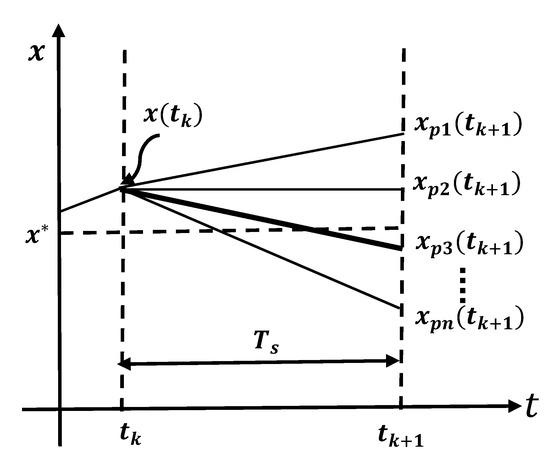
Figure 3.
An illustration showing the process of vector selection and estimation of MPC.
The discrete time model was derived from the predictive model directly and relies on the control parameters [43]. As a paradigm, for , the future predictive value at time can be determined from the measured value and for number of voltage vectors results in possible predictive values such as as shown in Figure 3. To determine the effectiveness of all possible voltage vectors on the system, a cost function was developed. The voltage vector that produced the minimum value of the cost function was selected for the next state. For instance, was the nearest value to the reference and, as a result, was selected during and instant.
2.2. Proposed Controller Modeling
Due to the widespread utilization in the commercial industry, the commonly used two-level voltage source inverter (VSI) was considered in the proposed system. The power circuit diagram of the three-phase, two-level inverter used in this work can be found in References [44,45]. The inverter was designed with IGBT switches, taking into account that the two switches in every inverter phase were working in the complementary mode to keep the dc source from short-circuiting. The switching states , , and of the inverter can be expressed as below [46].
Now, the vector form of can be expressed as [43]:
The total number of switching states will be the result of the different switching state combinations minus the impossible state. Here, the switching state that may be the reason for short-circuiting is defined as the impossible state. In general, the switching state’s number, , can be obtained as:
where the possible numbers of states are presented by of each leg, and presents the number of phases. For instance, a four-phase, three-level converter has switching states. If all the possible combinations are considered for a two-level, three-phase converter, eight possible voltage vectors are available. The voltage vectors can be represented in a two-dimensional plane and are shown in Figure 4 [47,48,49,50].
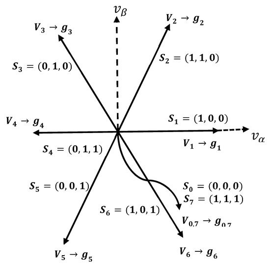
Figure 4.
Space distribution of all the admissible voltage vectors of the two-level voltage source inverter.
Taking into account the definitions of the variables of the three-phase, two-level inverter, the equations for output current dynamics for each phase can be written as [12]:
where is the line filter resistance and is the line filter inductance. Considering the space vector definition for the inverter voltage, the output current and grid voltage space vectors can be expressed as [12]:
The output voltage vector can be presented as:
Therefore, the dynamic output current equation can be expressed as:
and assuming the last term of Equations (6)–(8) equal to zero:
The output current dynamics can be described by the vector differential equation [12]:
In the proposed controller, a fixed amplitude and frequency grid voltage was considered. The output current derivative can be supplanted by a forward Euler approximation which can be presented as [51]:
Now, the predictive current at time can be expressed as:
where the grid voltage at time is denoted by .
2.3. Cost Function Design
The switching loss will eventually increase if the switching frequency is high, which also increases the overall losses. Therefore, the main purpose of the proposed controller was to reduce the loss as well as maintain the stability of the system. The possible switching movement in the next state in a three-phase, two-level inverter is shown in Figure 5. It is seen that the maximum switching commutation can be 3 and the minimum can be 0. The switching commutation can be determined by Equation (17) [36]:
where the current and the future predictive switching states are presented by and and is the index voltage vectors . For instance, if the current and future voltage vectors are (010) and (001), then and . Therefore, the switching commutation can be determined as follows:
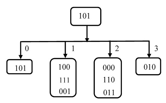
Figure 5.
Switching path action for the three-phase, two-level inverter.
The switching frequency reduction term, , can be added to the cost function in two ways. One is a single-cost function frequency reduction strategy and the second is a multi-cost function frequency reduction strategy [36]. The single-cost function strategy is simpler than the multi-cost function and efficient in reducing the switching frequency. Therefore, a single-cost function strategy was utilized in the research work during the design of the cost function.
The proposed cost function for the designed controller of this work was:
where is the real and is the imaginary component of current , respectively. The real and imaginary components of the predictive () and reference () currents are represented by , and , , respectively. The first term in Equation (19) is to reduce the reference tracking error. The term was added into the cost function which makes the difference of the proposed controller from the conventional MPC-based controller. The average switching frequency, , per switching device was determined by Equation (20) using the total number of switching transitions, , over the sampling time duration [52].
The switching state which yields the lowest number of commutation will be selected. Therefore, the use of in Equation (20) will have a direct effect on the switching frequency of the converter. The two terms in the cost function are combined by a weighting factor . The value of is determined by a heuristic process which suggests that the value of varies from 0 to below 1 and affects the controller. If the value of is larger, it emphasizes a greater value to the reduction of the switching frequency than the tracking error, and if lower, it emphasizes the reduction of the tracking error. Therefore, the value of is a crucial factor to maintain both the minimal value of switching frequency and tracking error at the same time, and hence, this phenomenon was carefully considered during the design of the controller.
2.4. Control Algorithm
The strategy utilized in the proposed controller can be sub-divided into five parts which were repeated several times until the optimal voltage vector was found and produced the minimum value for the cost function. After selecting the optimal vector, the newly selected vector was applied to the inverter. Therefore, to realize the control strategy, the five parts were: (i) assessment of the initial input parameters, (ii) calculation of controlling parameters, (iii) prediction of future behavior of the controlling parameters, (iv) making optimization between the calculated and predicted values, and (v) selection and application of the newly optimized value. The flowchart of the algorithm (shown in Figure 6) consisted of two loops: an inner and outer loop. For each of the seven different voltage vectors, the inner loop was executed, and the outer loop was executed at every sampling time for determining the optimal switching state related to the corresponding voltage vector. Therefore, the selected switching state for the optimized cost function was applied to the next sampling period. The five steps of implementing the control algorithm are presented in Algorithm 1 below.
| Algorithm 1. Algorithm utilized in the proposed controller |
| Input: Output: |
| 1. The inverter input voltage , output current , and grid voltage are measured. |
| 2. The future predictive current and the switching transitions from the immediate future state are calculated for all the possible eight states of the inverter using Equations (16) and (17), respectively. |
| 3. Estimation of the value of the proposed cost function using Equation (19). |
| 4. Selection of apposite switching state for the optimized cost function |
| 5. Application of the newly elected switching state to the next sampling state and return to Step 1. |
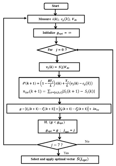
Figure 6.
Flowchart of the proposed predictive controller for selecting the optimal switching vector that implies minimal switching commutation.
3. Power Loss Analysis
The loss of power occurs due to the switching devices used in the circuit, which significantly influence the efficiency of the inverter [53,54,55]. The harmonic content in the output current and heat generated during the conduction of the switching device also provides a significant contribution to the overall loss of the system. Therefore, the overall loss of the system consists of conduction, switching, and harmonic loss. The conduction loss depends on the collector–emitter voltage and collector–current of the switching device. The inherent material used during the manufacturing of the switching device significantly affects the conduction loss. Hence, the reduction of the collector–emitter terminal voltage is the only way to lessen the conduction loss. Moreover, the temperature of the junction also influences the value of the losses. For estimating the average conduction loss, the following expressions were used [53,56].
where the threshold voltage and the differential resistance of the switching device (IGBT) are denoted by and , respectively. The value of them at a fixed temperature is collected from the datasheet provided by the manufacturer [57]. The value of output frequency was considered 50 Hz and was utilized to determine the value of as . Moreover, another value was needed, the upper IGBT arm current, which was denoted by . The following expression in Equations (23) and (24) were utilized to determine the value of and .
Equation (22) contains a term which is mainly dependent on the value of the modulation index. However, one benefit of FCS-MPC is that this method is free from the requirement of the modulation index. Hence, the value of is considered unity during the calculation. The turning on and off process of the switching device causes losses in the system that are referred to as switching loss. This loss is influenced by the input dc voltage and output current of the inverter, and by the variable parameters of the switching device. Besides, the terminal temperature of the device and resistance of the gate driver circuit affects the switching loss. To reduce the mentioned loss, several methods are available in the literature and mentioned in Table 2. For estimating the average switching loss, the following expressions are used [53,56].
where the switching frequency is presented by , is the inverter input voltage, and are the voltage across the collector–emitter terminal and the collector current of the switching device, respectively. From the datasheet provided by the manufacturer, the values of , , , and are collected [57]. The presence of THD or harmonics in the output current of the inverter leads to an extended power loss which is referred to as harmonic loss. Therefore, the THD of the injected grid current should be under the acceptable limit. As a result, to verify the performance of the proposed controller, the calculation of the harmonic loss is also necessary. Since the THD and switching frequency has an opposite effect on each other, there should be a trade-off between the harmonic and switching loss to have a lower overall loss in the system. The expressions in Equations (27) and (28) were utilized to determine the current THD () and harmonic loss of the proposed system [58].
where, , , and are the fundamental current, THD of the output current, and amount of current for the different harmonic components, respectively.
4. Results Analysis
A simulation of the proposed system, as well as the hardware realization of the blocks, was performed for the verification of the result. A 39 kW PV system was connected to the proposed controller-based inverter via a closed-loop boost converter. One hundred and sixty-eight modules having an individual capacity of 235 W were connected in a series and parallel connection to design the mentioned PV array. According to the simulation environment, a hardware prototype was considered for data acquisition and verification. The hardware system consisted of dc-link voltage provided by the PV system and a dc/dc converter, proposed MPC-based two-level, three-phase inverter, current sensor, a gate driver circuit, sensor connecting circuit, capacitor bank, desktop computer as a control desk, dSPACE 1104 as micro-processor, oscilloscope, R–L line filter, and the grid as shown in Figure 7. Table 3 presents the value of the parameters used in the presented work. For the inverter control platform, the dSPACE 1104 board was utilized, because it provided the linking between the real-time system to the MATLAB/Simulink model [59]. The dSPACE 1104 provided the linkage by utilizing its input/output interface such as DS1104_BIT_OUT_CX, DS1104ADC, DS1104DAC, etc. It converted the Simulink model to the C-code automatically by utilizing a built-in function named MATLAB/Simulink Real-Time Workshop (RTW) [60]. The converted C-code was then complied and made a linkage to the dSPACE board. A graphical user interface (GUI) software, named dSPACE ControlDesk, provided the real-time performance monitoring facility and also enabled to change the control variables and monitor the performance of the system in real-time. The dSPACE DS1104 real-time interface (RTI) implementation for generating the switching pulses for the proposed controller-based on-grid PV inverter is shown in Figure 8.
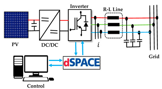
Figure 7.
Block diagram of the experimental setup for the proposed MPC-based controller for the on-grid PV inverter.
Table 3.
Parameter values for the simulated system.
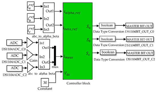
Figure 8.
The dSPACE DS1104 RTI implementation for generating switching pulses for the proposed controller-based, on-grid PV inverter.
The dSPACE DS1104ADC_CX block was utilized for taking the reading of the inverter output current which converts the currents into a digital form that is required by the controller. A current sensor, named “LA55p”, was used for sensing the output current of the inverter. Both the three-phase reference and measured current quantities were then transformed to coordinates for ease of control by using an to conversion block. For real-time implementation, the dc-link voltage was scaled down to 30 V instead of 850 V, and the other parameters were also changed with the apposite ratios. The switching signals generated by the controller were then delivered to the hardware (inverter) through a data type conversion “Boolean” block and a DS1104BIT_OUT_CX block. The controller generated only three switching signals (, , ) of the upper IGBTs, and the complements of them were generated by a gate driver named “IR2110” to provide the six required switching signals. The pictorial view of the implemented hardware of the proposed controller is shown in Figure 9.
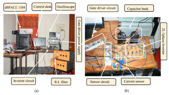
Figure 9.
Hardware prototype of the proposed system. (a) Complete setup of the environment for the experiment consisting of a control system and R–L filter circuit. (b) The gate driver circuit with the three-phase, two-level inverter is magnified.
The performance of the proposed controller in terms of steady-state analysis, current tracking accuracy, and the effect of adding the switching function in the cost function are described below.
4.1. Steady-State Analysis
The performance of the proposed controller was analyzed through steady-state analysis. The algorithm was implemented by the cost function as presented by Equation (19). The reference current utilized during the simulation was sinusoidal and having an amplitude of 96 A with a frequency of 50 Hz. The phase voltages () across the load before the LC filter is shown in Figure 10. Figure 11 shows the phase voltages () across the load after the LC filter.
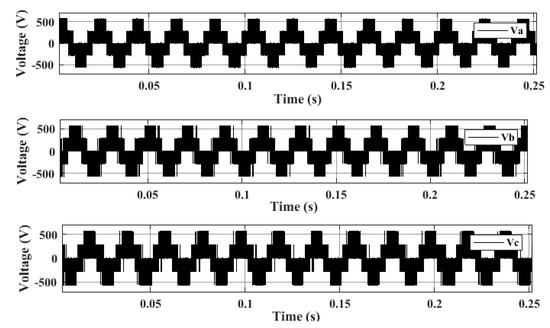
Figure 10.
Steady-state phase voltage () before the LC filter.
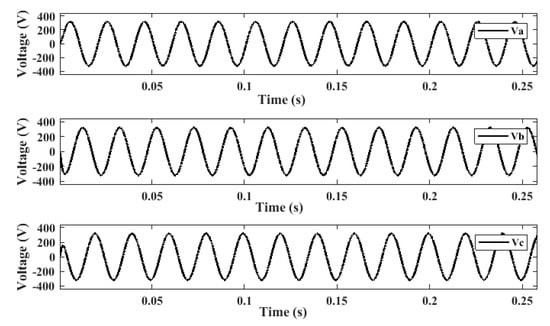
Figure 11.
Steady-state phase voltage () after the LC filter.
The steady-state, three-phase load currents () using the proposed controller are presented in Figure 12 which indicates a sinusoidal nature load current with low distortion.
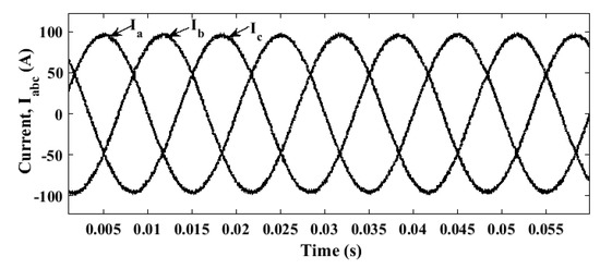
Figure 12.
Steady-state phase current waveforms () in the time domain.
4.2. Current Tracking Accuracy
The accuracy of the tracking output current of the proposed controller was checked by observing the behavior of the controller under steady-state and transient conditions. For evaluating the steady-state condition, a three-phase reference current was assumed to have an amplitude of 96 A and a frequency of 50 Hz. At time 0.015 s, a step reduction was done in the reference current (only in the real parameter ) by reducing it to half of its value for observing the transient behavior. The response of the output () and reference () current under the transient condition in the αβ frame was delineated in Figure 13. Figure 14 shows that the proposed controller provided a negligible mean absolute tracking error (MATE) at steady-state and transient conditions, which was only 0.025 (i.e., 2.5%). The MATE wasa determined by the following expression [23]:
where the reference and future predictive currents are indicated by and , respectively, to determine the MATE.
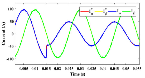
Figure 13.
The waveforms of output () and reference () current in the αβ frame under the transient condition.
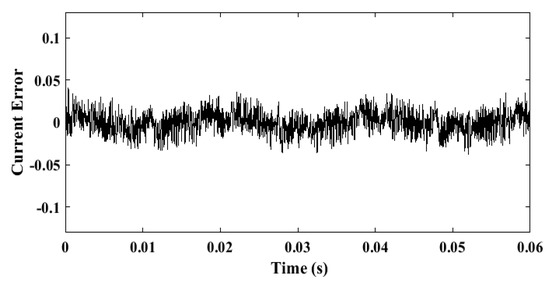
Figure 14.
Mean absolute tracking error between the measured and reference current.
Figure 14 suggests that during both the steady-state and transient conditions, the tracking accuracy of the controller was under the acceptable limit.
4.3. Effect of Switching Frequency Term in the Cost Function
As mentioned earlier, the cost function designed for the proposed controller included two components. One was for lessening the tracking error of the measured current and the other one was for lessening the switching transitions. The two terms were added with a weighting factor λ. Therefore, the value of λ is an important factor for determining an optimized cost function. For determining the effect of switching transitions reduction, the simulation of the whole system was done for λ = 0, i.e., neglecting the term in the cost function. Harmonic analysis was done for the output load current by using the fast Fourier transform (FFT) analysis and is shown in Figure 15, where the term “fundamental” denotes the desired frequency of the output current, which was 50 Hz, and the peak value of the output current with fundamental frequency was 95.97 A. In Figure 15, the illustration is zoomed in to show the contribution of the other frequency components, i.e., the harmonics in comparison with the fundamental frequency component. Thereafter, the r.m.s. value of the output current with a fundamental frequency was utilized to determine the THD of it using Equation (27). It can be seen that the current THD without the switching transitions reduction term was 1.82%. The experimentation was also performed with the addition of the switching frequency reduction terms in the cost function utilizing Equation (19). The value of weighting factor λ was varied over a range of 0.01 to 0.7, and the value of the switching frequency and the corresponding current THD are calculated and shown in Table 4. It can be seen that the switching frequency was 4.46 kHz and the corresponding current THD was 1.82% for λ = 0.
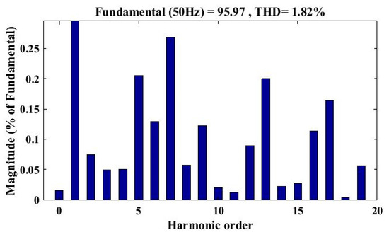
Figure 15.
Current THD without in the cost function.
Table 4.
Current THD, average switching frequency, and conduction and switching losses with the variation of the weighting factor, .
If the value of λ increased, the switching frequency decreased, while the current THD increased. For λ = 0.7, the switching frequency was 3.03 kHz which is the lowest one for the observed datasheet as shown in Table 4, while the current THD value was 2.38% which is the highest one. The current THD should be lower to having a lower harmonic loss. The switching frequency should also be lower for a lower switching loss in the semiconductor device. The switching frequencies, current THDs with the variation of λ are shown in Figure 16. It can be seen that the average switching frequency, , and the current THD curve intersected at , where the switching frequency was 3.54 kHz and the corresponding current THD was 2.07%.
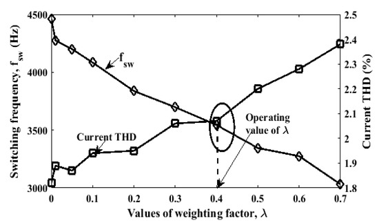
Figure 16.
Switching frequencies and current THDs with the variation of the weighting factor,. The trade-off point of was found to be 0.4.
It is noteworthy that, considering only 0.25% more current THD, the switching frequency was found to be a lower one. Hence, for energy-efficient operation of the inverter, it was operated at this trade-off point (i.e.,) of the average switching frequency and the current THD. The steady-state current response of the output load current with is shown in Figure 17. Figure 17 indicates that the waveform did not change much from the waveform for .
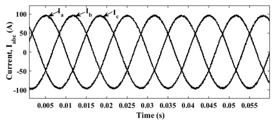
Figure 17.
Steady-state phase currents () using the proposed controller for .
5. Comparison with Conventional MPC
For the value of , a loss analysis was conducted. The utilized value of the power loss analysis parameters is presented in Table 5. At that condition, the instantaneous behavior of switching and conduction loss is delineated in Figure 18, using Equations (22) and (26), respectively. The average value of the switching, conduction, and harmonic losses are calculated for both the proposed and conventional controller and are shown in Figure 19.
Table 5.
Parameters for the power loss analysis [2,57].
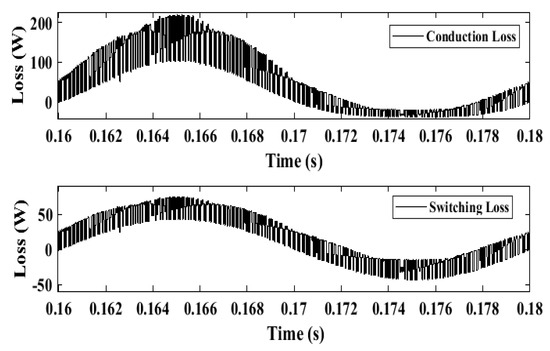
Figure 18.
Waveforms of the instantaneous conduction and switching losses in MPC using Equations (22) and (26) respectively.
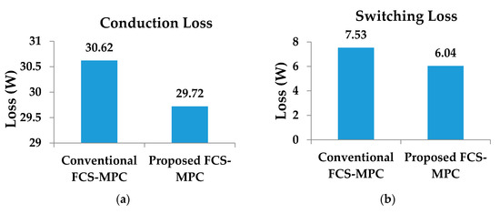
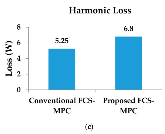
Figure 19.
(a) Conduction, (b) switching, and (c) harmonic loss in the conventional FCS-MPC and the proposed FCS-MPC based controller.
From Figure 19a, the continuous conduction losses per phase of a three-phase system were 30.62 W and 29.72 W for the conventional FCS-MPC and proposed FCS-MPC, respectively. Therefore, it can be said that 3% conduction loss was reduced due to the addition of in the cost function. From Figure 19b, the continuous switching losses per phase of a three-phase system were 7.53 W and 6.04 W for the conventional FCS-MPC and proposed FCS-MPC, respectively. It can be seen that a 19.78% loss was reduced due to the addition of . The harmonic loss was also calculated for the same case and is shown in Figure 19c. It is noted that the continuous harmonic losses calculated up to 19th harmonics with and without were 6.79 W and 5.25 W, respectively. Hence, the proposed system suffers from 1.54 W due to the trade-off of the current THD and switching frequency as shown in Figure 19c.
The contribution of conduction, switching and harmonic loss per phase in percentage for conventional and proposed MPC-based controllers are shown in Figure 20. It can be seen that the conduction and switching loss was reduced by 0.72% and 3.33% per phase in the proposed controller than the conventional controller. A 3.86% more harmonic loss per phase was considered in the proposed controller to reach the optimal point of the weighting factor. Although the proposed controller suffered from a slightly higher harmonic loss, it provided a lower overall loss than the conventional MPC.
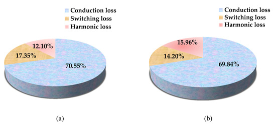
Figure 20.
The contribution of conduction, switching, and harmonic loss per phase in percentage in the (a) conventional FCS-MPC and (b) the proposed FCS-MPC based controller.
Now, the comparison between the conventional FCS-MPC based controller and the proposed controller is shown in Table 6, which highlights the reduction of switching frequency, switching loss, and the overall power loss of the system instead of using the conventional FCS-MPC based controller. It is seen that the total per phase continuous loss for the conventional FCS-MPC and proposed FCS-MPC were 43.40 W and 42.56 W, respectively. Therefore, 0.84 W was reduced per phase due to the switching frequency reduction. For the three-phase system, the total reduced loss is (0.84 3) = 2.52 W, which shows a significant amount of loss reduction due to the incorporation of in the cost function.
Table 6.
Comparison of the proposed controller with conventional FCS-MPC based controller.
To verify the performance of the proposed controller, the chosen reference current (96 A) varied over a range of 91 to 100 A, and each time the conduction and switching loss was determined (as shown in Figure 21). The linear variation of both the losses ensured that the losses did not depend on the variation of reference parameters.
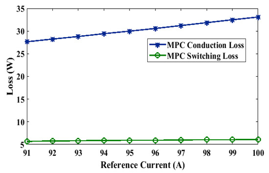
Figure 21.
Comparison of conduction and switching losses of MPC based controller during the variation of the reference current.
6. Conclusions
For penetrating maximum power to the grid and to reduce the overall loss of the system, an on-grid inverter controlling was proposed based on the MPC method. The proposed controller was first designed in the MATLAB/Simulink platform and then small-scale hardware was realized to verify it. For lessening the tracking error of the output current and switching loss, an effective cost function was designed with an apposite weighting factor. The performance of the proposed MPC was observed with and without a switching frequency reduction term () in the cost function. The tracking error was found at 2.5% during the steady-state and transient conditions, which is under the considerable limit. The current THD, average switching frequency, and switching loss were 1.82%, 4.46 kHz, and 7.53 W, respectively, without . After adding in the cost function, the current THD, switching frequency, and the switching loss became 2.07%, 3.54 kHz, and 6.05 W, respectively, with a weighting factor of . This means that the average switching frequency was reduced by 20.62% (920 Hz) and the corresponding switching loss was reduced by 19.78% (1.49 W) per phase, while the current THD increased by only 0.25%. The overall loss of the inverter was also calculated. It was shown that the overall losses for the proposed and conventional controller were 42.56 and 43.40 W, respectively, considering only 0.25% more current THD had minimized the average switching loss as well as reduced the continuous overall losses by 2% (for the three-phase). The experiment could also be conducted with AC-tied energy storage inverter, the analysis, and the results of which will be explored in-depth in future research.
Author Contributions
All authors have equally contributed to this work. All authors have read and agreed to the published version of the manuscript.
Funding
This research received no external funding.
Conflicts of Interest
The authors declare no conflict of interest.
Nomenclature
| CCS | Continuous Control Set |
| DTC | Direct Torque Control |
| FCS-MPC | Finite Control Set Model Predictive Control |
| FFT | Fast Fourier Transform |
| IGBT | Insulated Gate Bipolar Transistor |
| MATE | Mean Absolute Tracking Error |
| MPC | Model Predictive Control |
| MPPT | Maximum Power Point Tracking |
| MPDPC | Model Predictive Direct Power Control |
| MPDCC | Model Predictive Direct Current Control |
| PV | Photovoltaic |
| PR | Proportional Resonant |
| PI | Proportional Integral |
| PWM | Pulse Width Modulation |
| P&O | Perturb and Observe |
| SMC | Sliding Mode Control |
| SVM | Space Vector Modulation |
| THD | Total Harmonic Distortion |
| VSI | Voltage Source Inverter |
| , , and | IGBT switching states |
| Future predictive load transitions | |
| Measured parameters | |
| Reference parameter | |
| Step-size of the model | |
| Switching state number | |
| Number of phases | |
| Output voltage vector | |
| DC link voltage | |
| Load current | |
| Grid electromotive force | |
| Cost function | |
| Grid voltage | |
| and | Real and imaginary components of the output current |
| Future predictive current | |
| Number of transitions of the switching devices | |
| Sampling time duration | |
| Switching frequency | |
| Weighting factor | |
| Optimal voltage vector | |
| selected switching state | |
| IGBT turn-on/threshold voltage | |
| IGBT differential resistance | |
| Average conduction loss | |
| Instantaneous conduction loss | |
| Average switching loss | |
| Instantaneous switching loss | |
| Arm current through the upper IGBT | |
| Collector-emitter terminal voltage | |
| Collector current | |
| Turn-on energy | |
| Turn-off energy | |
| Fundamental current | |
| Harmonic component current | |
| Value of current THD | |
| Harmonic loss | |
| Line filter resistance | |
| Output frequency | |
| Phase voltages | |
| Phased currents | |
| , | Phase currents in domain |
References
- Podder, A.K.; Habibullah, M.; Roy, N.K. Current THD analysis of model predictive control based grid-connected PV inverter. In Proceedings of the International Conference on Electrical, Computer and Communication Engineering (ECCE), Cox’s Bazar, Bangladesh, 7–9 February 2019; pp. 1–6. [Google Scholar]
- Podder, A.K.; Tariquzzaman, M.; Habibullah, M. Comprehensive performance analysis of model predictive current control based on-grid photovoltaic inverters. J. Phys. Conf. Ser. 2020, 1432, 1–11. [Google Scholar] [CrossRef]
- Holtz, J. Pulsewidth modulation for electronic power conversion. Proc. IEEE 1994, 82, 1194–1214. [Google Scholar] [CrossRef]
- Mohamed, I.S.; Zaid, A.; Abu-Elyazeed, M.F.; Elsayed, H.M. Model predictive control and classical methods for UPS inverter applications with output LC filter. In Proceedings of the 2013 International Conference on Control, Decision and Information Technologies (CoDIT), Hammamet, Tunisia, 6–8 May 2013; pp. 483–488. [Google Scholar]
- Parvez, M.; Elias, M.F.M.; Rahim, N.A. Analysis of current harmonics compensation and the effect of frequency variation for single-phase stand-alone PV inverters using PR controller. IETE J. Res. 2017, 64, 463–470. [Google Scholar] [CrossRef]
- Escobar, G.; Valdez, A.A.; Leyva-Ramos, J.; Mattavelli, P. Repetitive-based controller for a UPS inverter to compensate unbalance and harmonic distortion. IEEE Trans. Ind. Electron. 2007, 54, 504–510. [Google Scholar] [CrossRef]
- Kojima, M.; Hirabayashi, K.; Kawabata, Y.; Ejiogu, E.C.; Kawabata, T. Novel vector control system using deadbeat-controlled PWM inverter with output LC filter. IEEE Trans. Ind. Appl. 2004, 40, 162–169. [Google Scholar] [CrossRef]
- Sebaaly, F.; Vahedi, H.; Kanaan, H.Y.; Moubayed, N.; Al-Haddad, K. Design and implementation of space vector modulation-based sliding mode control for grid-connected 3L-NPC inverter. IEEE Trans. Ind. Electron. 2016, 63, 7854–7863. [Google Scholar] [CrossRef]
- Saeedifard, M.; Bakhshai, A.; Joos, G. Low switching frequency space vector modulators for high power multi-module converters. IEEE Trans. Power Electron. 2015, 20, 1310–1318. [Google Scholar] [CrossRef]
- Gopinath, A.; Mohamed, A.; Baiju, M.R. Fractal based space vector PWM for multilevel inverters—A novel approach. IEEE Trans. Ind. Electron. 2019, 56, 1230–1237. [Google Scholar] [CrossRef]
- Aneesh, M.; Gopinath, A.; Baiju, M.R. A simple space vector PWM generation scheme for any general n–level inverter. IEEE Trans. Ind. Electron. 2019, 56, 1649–1656. [Google Scholar]
- Rodrguez, J.; Pontt, J.; Silva, C.A.; Correa, P.; Corts, P.; Ammann, U. Predictive current control of a voltage source inverter. IEEE Trans. Ind. Electron. 2007, 54, 495–503. [Google Scholar] [CrossRef]
- Cortes, P.; Kazmierkowski, M.P.; Kennel, R.M.; Quevedo, D.E.; Rodriguez, J. Predictive control in power electronics and drives. IEEE Trans. Ind. Electron. 2008, 55, 4312–4324. [Google Scholar] [CrossRef]
- Lee, J.H. Model predictive control: A review of the three decades of development. Int. J. Control Automat. Syst. 2011, 9, 415–424. [Google Scholar] [CrossRef]
- Morariand, M.; Lee, J.H. Model predictive control: Past, present, and future. Comput. Chem. Eng. 1999, 23, 667–682. [Google Scholar] [CrossRef]
- Kouro, S.; Cortes, P.; Vargas, R.; Ammann, U.; Rodríguez, J. Model predictive control—A simple and powerful method to control power converters. IEEE Trans. Ind. Electron. 2009, 56, 1826–1838. [Google Scholar] [CrossRef]
- Podder, A.K.; Habibullah, M. Model predictive based energy-efficient control of grid-connected PV system. In Proceedings of the 10th International Conference on Electrical and Computer Engineering (ICECE 2018), Dhaka, Bangladesh, 20–22 December 2018; pp. 413–416. [Google Scholar]
- Vazquez, S.; Leon, J.I.; Franquelo, L.G.; Rodriguez, J.; Young, H.A.; Marquez, A.; Zanchetta, P. Model predictive control: A review of its applications in power electronics. IEEE Ind. Electron. Mag. 2014, 8, 16–31. [Google Scholar] [CrossRef]
- Kazmierkowski, M.P.; Malesani, L. Current control techniques for three-phase voltage-source PWM converters: A survey. IEEE Trans. Ind. Electron. 1998, 45, 691–703. [Google Scholar] [CrossRef]
- Timbus, A.; Liserre, M.; Teodorescu, R.; Rodriguez, P.; Blaabjerg, F. Evaluation of current controllers for distributed power generation systems. IEEE Trans. Power Electron. 2009, 24, 654–664. [Google Scholar] [CrossRef]
- Chen, X.; Wu, W.; Gao, N.; Liu, J.; Chung, H.S.-H.; Blaabjerg, F. Finite control set model predictive control for an LCL-filtered grid-tied inverter with full status estimations under unbalanced grid voltage. Energies 2019, 12, 2691. [Google Scholar] [CrossRef]
- Ahmed, A.A.; Koh, B.K.; Lee, Y.I. Continuous control set-model predictive control for torque control of induction motors in a wide speed range. Electr. Power Compon. Syst. 2018, 46, 2142–2158. [Google Scholar] [CrossRef]
- Ngo, V.-Q.-B.; Nguyen, M.-K.; Tran, T.-T.; Choi, J.-H.; Lim, Y.-C. A modified model predictive power control for grid-connected T-type inverter with reduced computational complexity. Electronics 2019, 8, 217. [Google Scholar] [CrossRef]
- Xia, C.; Liu, T.; Shi, T.; Song, Z. A simplified finite-control-set model-predictive control for power converters. IEEE Trans. Ind. Inform. 2014, 10, 991–1002. [Google Scholar]
- He, F.; Zhao, Z.; Lu, T.; Yuan, L. Predictive DC voltage control for three-phase grid-connected PV inverters based on energy balance modeling. In Proceedings of the 2nd International Symposium on Power Electronics for Distributed Generation Systems, Hefei, China, 16–18 June 2010; pp. 516–519. [Google Scholar]
- Jianhua, W.; Jing, Z.; Longfei, L.; Cong, T.; Le, Y. Predictive control based on analytic model for PV grid-connected inverters. In Proceedings of the 24th Chinese Control and Decision Conference (CCDC), Taiyuan, China, 23–25 May 2012; pp. 4295–4299. [Google Scholar]
- Nan, J.; Xuanxuan, D.; Guangzhao, C.; Zhifeng, D.; Dongyi, K. Model-predictive direct power control of grid-connected inverters for PV systems. In Proceedings of the International Conference on Renewable Power Generation (RPG), Beijing, China, 17–18 October 2015; pp. 1–5. [Google Scholar]
- Nan, J.; Shiyang, H.; Guangzhao, C.; Suxia, J.; Dongyi, K. Model-predictive current control of grid-connected inverters for PV systems. In Proceedings of the International Conference on Renewable Power Generation (RPG), Beijing, China, 17–18 October 2015; pp. 1–5. [Google Scholar]
- Shang, L.; Li, P.; Li, Z. Low voltage ride through control method of photovoltaic grid-connected inverter based on model current predictive control. In Proceedings of the Chinese Control and Decision Conference (CCDC), Shenyang, China, 9–11 June 2018; pp. 5209–5214. [Google Scholar]
- Bighash, E.Z.; Sadeghzadeh, S.M.; Ebrahimzadeh, E.; Blaabjerg, F. Robust MPC-based current controller against grid impedance variations for single-phase grid-connected inverters. ISA Trans. 2019, 84, 154–163. [Google Scholar] [CrossRef]
- Bighash, E.Z.; Sadeghzadeh, S.M.; Ebrahimzadeh, E.; Blaabjerg, F. High-quality model predictive control for single phase grid-connected photovoltaic inverters. Elec. Power Syst. Res. 2018, 158, 115–125. [Google Scholar] [CrossRef]
- Geldenhuys, J.M.C. Model Predictive Control of a Grid-Connected Converter with LCL-Filter. Master’s Thesis, University of Stellenbosch, Stellenbosch, South Africa, 2018. [Google Scholar]
- Roh Chan, R.; Kwak, S. Model-based predictive current control method with constant switching frequency for single-phase voltage source inverters. Energies 2017, 10, 1927. [Google Scholar] [CrossRef]
- Kwak, S.; Park, J. Switching strategy based on model predictive control of VSI to obtain high efficiency and balanced loss distribution. IEEE Trans. Power Electron. 2014, 29, 4551–4567. [Google Scholar] [CrossRef]
- Vargas, R.; Ammann, U.; Rodriguez, J.; Pontt, J. Reduction of switching losses and increase in efficiency of power converters using predictive control. In Proceedings of the IEEE Power Electronics Specialists Conference, Rhodes, Greece, 15–19 June 2008; pp. 1062–1068. [Google Scholar]
- Cui, Q.; Liao, M.; Liao, Z.; Chen, Z. Frequency reduction-based model predictive direct power control with multi-cost function. Adv. Intell. Syst. Res. 2018, 143, 241–245. [Google Scholar]
- Preindl, M.; Schaltz, E.; Thogersen, P. Switching frequency reduction using model predictive direct current control for high-power voltage source inverters. IEEE Trans. Ind. Electron. 2011, 58, 2826–2835. [Google Scholar] [CrossRef]
- Hu, J.; Zhu, J.; Dorrell, D.G. Model predictive control of grid-connected inverters for PV systems with flexible power regulation and switching frequency reduction. IEEE Trans. Ind. App. 2015, 51, 587–594. [Google Scholar] [CrossRef]
- Yaramasu, V.; Wu, B.; Rivera, M.; Rodriguez, J. Enhanced model predictive voltage control of four-leg inverters with switching frequency reduction for standalone power systems. In Proceedings of the 15th International Power Electronics and Motion Control Conference (EPE/PEMC), Novi Sad, Serbia, 4–6 September 2012; pp. DS2c.6-1–DS2c.6-5. [Google Scholar]
- Abushaiba, A.A.; Eshtaiwi, S.M.M.; Ahmadi, R. A new model predictive based maximum power point tracking method for photovoltaic applications. In Proceedings of the International Conference on Electro Information Technology (EIT), Grand Forks, ND, USA, 19–21 May 2016; pp. 0571–0575. [Google Scholar]
- Podder, A.K.; Roy, N.K.; Pota, H.R. MPPT methods for solar PV systems: A critical review based on tracking nature. IET Renew. Power Gen. 2019, 13, 1615–1632. [Google Scholar] [CrossRef]
- Hu, J.; Cheng, K.W.E. Predictive control of power electronics converters in renewable energy systems. Energies 2017, 10, 515. [Google Scholar] [CrossRef]
- Rodriguez, J.; Cortes, P. Predictive Control. of Power Converters and Electrical Drives; Wiley-IEEE: Hoboken, NJ, USA, 2012. [Google Scholar]
- Habibullah, M. Simplified Finite-State Predictive Torque Control Strategies for Induction Motor Drives. Ph.D. Thesis, The University of Sydney, Sydney, Australia, 2016. [Google Scholar]
- Shuvo, S.; Hossain, E.; Islam, T.; Akib, A.; Padmanaban, S.; Khan, M.Z.R. Design and hardware implementation considerations of modified multilevel cascaded H-Bridge inverter for photovoltaic system. IEEE Access 2019, 7, 16504–16524. [Google Scholar] [CrossRef]
- Kennel, R.; Schronder, D. Predictive control strategy for converters. In Proceedings of the 3rd IFAC Symposium on Control in Power Electronics and Electrical Drives, Lausanne, Switzerland, 12–14 September 1983; pp. 415–422. [Google Scholar]
- Rodriguez, J.; Kazmierkowski, M.P.; Espinoza, J.R.; Zanchetta, P.; Abu-Rub, H.; Young, H.A.; Rojas, C.A. State of the art of finite control set model predictive control in power electronics. IEEE Trans. Ind. Inform. 2013, 9, 1003–1016. [Google Scholar] [CrossRef]
- Jun, E.; Park, S.; Kwak, S. Model predictive current control method with improved performances for three-phase voltage source inverters. Electronics 2019, 8, 625. [Google Scholar] [CrossRef]
- Malek, H. Control of Grid-Connected Photovoltaic Systems Using Fractional-Order Operators. Ph.D. Thesis, Utah State University, Logan, UT, USA, 2014. Available online: https://digitalcommons.usu.edu/etd/2157 (accessed on 24 January 2020).
- Buso, S.; Mattavelli, P. Digital Control. In Power Electronics; (Ser. 978-1598291124); Morgan and Claypool Publishers: Denver, CO, USA, 2006. [Google Scholar]
- Blaabjerg, F.; Chen, Z.; Kjaer, S. Power electronics as efficient interface in dispersed power generation systems. IEEE Trans. Power Electron. 2004, 19, 1184–1194. [Google Scholar] [CrossRef]
- Perantzakis, G.; Xepapas, F.; Papathanassiou, S.; Manias, S. A predictive current control technique for three-level NPC voltage source inverters. In Proceedings of the IEEE Power Electronics Specialists Conference, Recife, Brazil, 12–16 June 2005; pp. 1241–1246. [Google Scholar]
- Zhang, Z.; Wang, H.; Wang, Z.; Yang, Y.; Blaabjerg, F. Simplified thermal modeling for IGBT modules with periodic power loss profiles in modular multilevel converters. IEEE Trans. Ind. Electron. 2019, 66, 2323–2332. [Google Scholar] [CrossRef]
- Qin, R.; Yang, C.; Tao, H.; Peng, T.; Yang, C.; Chen, Z. A power loss decrease method based on finite set model predictive control for a motor emulator with reduced switch count. Energies 2019, 12, 4647. [Google Scholar] [CrossRef]
- Alhasheem, M.; Blaabjerg, F.; Davari, P. Performance assessment of grid forming converters using different finite control set model predictive control (FCS-MPC) algorithms. Appl. Sci. 2019, 9, 3513. [Google Scholar] [CrossRef]
- Bierhoff, M.H.; Fuchs, F.W. Semiconductor losses in voltage source and current source IGBT converters based on analytical derivation. In Proceedings of the 35th Annual Power Electronics Specialists Conference (IEEE Cat. No.04CH37551), Aachen, Germany, 20–25 June 2004; pp. 2836–2842. [Google Scholar]
- On Semiconductor. “IGBT” NJTG50N60FWG Datasheet. December 2012. Available online: https://www.onsemi.com/pub/Collateral/NGTG50N60FW-D.PDF (accessed on 4 April 2020).
- Ghorbani, M.J.; Mokhtari, H. Impact of harmonics on power quality and losses in power distribution systems. Int. J. Electr. Comput. Eng. (IJECE) 2015, 5, 166–174. [Google Scholar] [CrossRef]
- Ghani, Z.A.; Hannan, M.A.; Mohamed, A. Renewable energy inverter development using dSPACE DS1104 controller board. In Proceedings of the IEEE International Conference on Power and Energy (PECon2010), Kuala Lumpur, Malaysia, 29 November–1 December 2010; pp. 1–6. [Google Scholar]
- dSPACE DS1104. Hardware Installation and Configuration and ControlDesk Experiment Guide; dSPACE GmbH: Paderborn, Germany, 2008; Available online: https://datacenterhub.org/dv_dibbs/file/1333:dibbs/?f=/1333/data/files/experiments/reports/106885/DS1104_config.pdf (accessed on 30 October 2019).
© 2020 by the authors. Licensee MDPI, Basel, Switzerland. This article is an open access article distributed under the terms and conditions of the Creative Commons Attribution (CC BY) license (http://creativecommons.org/licenses/by/4.0/).