Preventive Maintenance and Forced Outages in Power Plants in Korea

Abstract

Maintaining high facility reliability in power plants is essential to secure long-term electricity supply. This paper applies the survival analysis to the actual unit level power generation data in Korea to estimate the relationship between facility reliability and the preventive maintenance. Duration of generators between forced outages is used to measure plant reliability. the empirical analysis shows that preventive maintenance cost, planned outage for maintenance, use rate, and reserve margin lead to the longer duration of generators and, in turn, the lower forced outage rates. We uncover that the marginal benefit of the preventive maintenance cost is decreasing at an increasing rate. It indicates that the marginal benefit of the “current” maintenance cost is minimal. Results in the paper imply that power plants in Korea might be spending unnecessarily high maintenance costs considering already having world’s lowest forced outage rates.

1. Introduction

Energy security, securing a long-term electricity supply, is indispensable to meet any changes in electricity demand. Additional generation capacity above the expected peak load, so-called reserve margin, is required to make electricity available for consumers at all times. As such, it is essential to equip sufficient generation capacity and maintain high facility reliability in power plants. It is typically important to the Republic of Korea (Korea, hereafter) since its electric grid is isolated, i.e., there is no cross-border power grid interconnected to Korea due to the geo-political characteristics. Note that Korea is located on the Korean Peninsula in Northeast Asia between China (to the west with the Yellow Sea) and Japan (to the southeast with East Sea and Korea Straight). North Korea is located to the north of Korea where the grid is disconnected. The Korean government has made the long-term electricity supply plan and set the reserve margin target to be 22% of annual peak load [1] which would meet any abrupt increases in electricity demand. Please note that the reserve margin of 22% is much higher than the typical reserve margin in other countries ranging from 12–15% as reported in [2].

Maintaining the high reserve margin requires the reliability of power generators. The Korean government obliges the Korea Electric Power Corporation (KEPCO), which is the government investment company being responsible for the transmission and distribution of electricity, to maintain a high degree of facility reliability based on Articles 18 and 25 in the Korean Electricity Utility Act. Please note that most of Korea’s generating capacities are controlled by the KEPCO like its subsidiaries as the Korean government owns 51% share of the KEPCO directly and indirectly. According to All Public Information In-One (ALIO, www.alio.go.kr) which is the public management information system in Korea, as of 2020, 51% of KEPCO shares is owned by the Ministry of Trade, Industry, and Energy (MTIE, 18.2%) and Korea Development Bank (KDB, 32.9%) [3]. According to “Eighth Basic Plan for Long-term Electricity Demand-Supply” prepared by the Ministry of Trade, Industry and Energy [1], the Korean government has targeted the loss of load expectation (LOLE) of 0.3 days/year. The LOLE represents the number of hours per annum in which over the long-term, it is expected statistically that supply will not meet demand. The LOLE of 0.3 days/year implies a 3-day disruption in electricity supply every ten years. Closely related to the LOLE, the Forced Outage Factor (FOF (%) = $\frac{\mathrm{unplanned}\mathrm{outage}\mathrm{in}\mathrm{hours}}{365\mathrm{days}(=8760\mathrm{h})}$) is the rate that the power station unit will not be available for service when required; it has been kept less than 1% which is much smaller than 4–5% rates reported in North American Electric Reliability Corporation (NERC). Similar to the FOF, the Unplanned Capability Loss Factor (UCLF (%) = $\frac{\mathrm{elec}.\mathrm{that}\mathrm{wasn}’\mathrm{t}\mathrm{produced}\mathrm{during}\mathrm{unplanned}\mathrm{shutdown}\mathrm{and}\mathrm{forced}\mathrm{outage}\mathrm{in}\mathrm{MWh}}{\mathrm{elec}.\mathrm{that}\mathrm{could}\mathrm{be}\mathrm{produced}\mathrm{if}\mathrm{the}\mathrm{unit}\mathrm{were}\mathrm{operated}\mathrm{continuously}\mathrm{at}\mathrm{full}\mathrm{power}}$) is the ratio of the unplanned energy losses during a given period of time, to the reference electricity generation. Unplanned energy loss is energy that was not produced during the period of unplanned shutdowns, forced outages, or unplanned load reductions due to plant management control. The lower FOF implies the lower UCLF and vice versa.

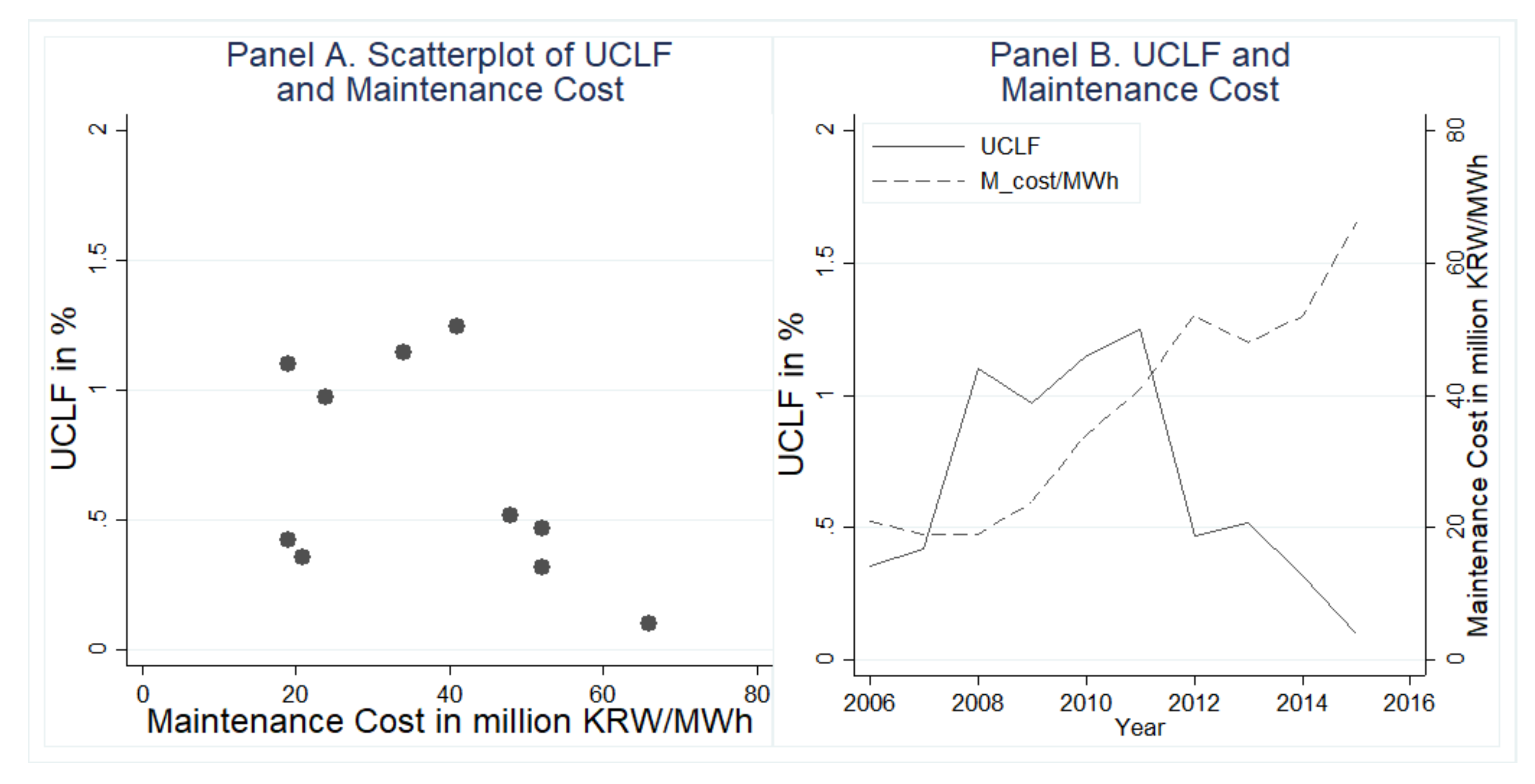
Panel A in Figure 1 presents the relationship between the actual plant level UCLF and the preventive maintenance. Maintenance is the actions need to be taken to ensure that a power plant generates reliable electricity; according to [4], there are two types of maintenance, (i) reactive or corrective maintenance which is carried out when the generator fails and (ii) preventive or predictive maintenance which is regularly scheduled inspections, tests, repairs and replacement of components; it will extend the generator life, reduce premature failures and increase the generator availability [4]. We focus on preventive maintenance in this article. In a power plant, which is named as “Plant A” due to the data confidentiality. As shown in Panel a in Figure 1, spending more preventive maintenance cost lowers the UCLF as expected. Since 2009, Plant a increased the preventive maintenance cost and it has been raised substantially after 2011 when the nationwide blackout hit Korea. Plant a spent 66 million KRW/MWh (roughly $60,000/MWh) in 2015, while the average of maintenance cost between 2005 and 2010 was only 23 million KRW/MWh (roughly $20,000/MWh) (Panel B in Figure 1). Since 2012, Plant a has kept the UCLF less than 0.6% and even the UCLF became 0.1% in 2015. It is 10 to 50 times smaller than the UCLF of 5% reported in NERC.

As alluded in Figure 1, power plants in Korea spend unnecessarily high preventive maintenance cost to keep the UCLF extremely low compared to other countries. A question is whether it is socially optimal. The high UCLF leads to a decrease in direct electricity sales and also incurs costs that require to operate expensive generators to meet the electricity demand, which in turn, causes the high social costs [5,6]. Spending high preventive maintenance cost to keep the UCLF unnecessarily low could be the waste, which is socially inefficient. Two research questions have emerged consequently as follows:

• What is the relationship between plant reliability in power generation and the preventive maintenance cost? We expect, of course, that spending more preventive maintenance cost increases the facility reliability and
• What is the marginal benefit of spending more preventive maintenance cost? Are power plants in Korea spending unnecessarily high preventive maintenance cost? This paper demonstrates that the marginal benefit of maintenance cost at current level is pretty low. It is an important question since the Korean government has been using the UCLF for power plants’ performance assessment, which may have caused power plants to spend unnecessarily high preventive maintenance cost.

Please note that in the empirical analysis, forced outage rate and duration of generators without forced outage are used as the proxies of the UCLF, which are also the measures of the power plant’s reliability and quality. Forced outage rate is slightly different from FOF, which is defined in this paper as following

$$\mathrm{forced}\mathrm{outage}\mathrm{rate}(\%)=\frac{\mathrm{forced}\mathrm{outage}\mathrm{in}\mathrm{hours}\times 100}{\mathrm{duration}\mathrm{without}\mathrm{outage}\mathrm{in}\mathrm{hours}+\mathrm{forced}\mathrm{outage}\mathrm{in}\mathrm{hours}}$$

(1)

To answer the questions above, we adopt the survival analysis and estimate the relationship between duration of generators and preventive maintenance. The survival analysis or duration analysis is a popular data analysis approach for certain kinds of data for which the outcome variable of interest is time until an event occurs [7]. the survival approach is appropriate since the duration between forced outages is a random variable in the sense that it represents the duration or the waiting time until the failure of the generator, i.e., forced outage, and we do not know the duration or the waiting time exactly; it is known as censoring or incomplete information [7]. In other words, some of the generators have no forced outages in the sample period. In addition, the duration until the generator failure is not normally distributed. Both censoring and non-normality generate difficulty when we analyze the data using the traditional statistical models such as multiple linear regression [8].

To the best of authors’ knowledge, this type of the study has been rare in the energy policy and economics literature, especially using the actual unit level power generation data; it makes this paper unique and significant. As will be discussed in the literature review section, in [9] is the only similar study identified. Other than the literature in energy policy and economics, there have been numerous studies about forecasting and managing forced outage rates using analytical methods or simulations in Engineering literature to improve power system reliability. As also will be discussed in result section, the marginal benefit of the preventive maintenance at current level in Korea is minimal implying that, policy-wise, Korean power plants are spending unnecessarily high preventive maintenance cost to keep the UCLF extremely low.

2. Literature Review

As generation facilities in power system age, the probability of forced outage increases gradually leading to a decline in generation system reliability. Thus, regular preventive maintenance is inevitable including planned outages [10]. To the best of the authors’ knowledge, there has been no study of power plants’ reliability and the preventive maintenance cost using the actual power plants’ internal unit level data perhaps because of data availability. [9], which is similar to this study, examined whether the higher use rates of generators, due to California electricity crisis of 2000–2001, had contributed to the higher (forced) outage rates. Using the data from the Mirant power plant, they showed that the higher use should increase outage rates.

In [11] is not closely related to the present study but investigated the factors that explain the substantial increase in wholesale electricity price in California during the summer of 2000. The authors found that there is a large gap between their simulated prices and observed prices, suggesting that the prices observed during summer 2000 reflect, in part, the exercise of market power by suppliers. In doing this, they analyzed the impact of forced outage on the electricity supply using actual generation data.

There have been, however, a series of studies related to preventive maintenance and its scheduling, generator reliability and forecasting forced outage rates using analytical methods, simulation, mathematical programming techniques in engineering literature to improve power system reliability. A few such studies are discussed here. As said in [12], generator maintenance is important factor that affects the profit from power plants. Turbines, combustors and electronic controllers in a power plant should be inspected periodically to minimize possible breakdowns and malfunctions during normal running and retain the reliability [12]. For this matter, there is an extensive literature, so-called Generation Maintenance Scheduling problem which determines the period for which generating units should be stopped for preventive maintenance. It varies in the objective which might be profit maximization [13], system reliability maximization [14], maintenance cost minimization [15,16] or multi objectives [17]. Many of studies have built an optimization models such as mathematical programming techniques, for planning preventive maintenance schedule.

Another vein of study is to assess the reliability of power generating plants since the availability of reliable power supply is important. Assessing the reliability power generation system usually done through simulation or analytical methods with the various reliability indices, for example, loss of load frequency, loss of energy expectation, and loss of load expectation [18]. Simulation techniques may result in high computational burden in complex system [19]. Many studies have used analytic techniques such as universal generating function [19,20,21] and iterative numerical technique [22]. Related to assessment of the system reliability, looking for a way to optimally use the available generation resources has interested many research in the electric power system operation as well [23] with the advent of innovative ideas to utilize the renewable energy recently [24].

3. Empirical Model

The survival analysis or duration analysis is a popular data analysis approach for certain kinds of data for which the outcome variable of interest is time until an event occurs [7]. The survival analysis is employed to empirically estimate the relationship between operation hours of generators or forced outages and the preventive management; it is because the duration between forced outages is a random variable in the sense that it represents the waiting time until the occurrence of an event, failure of the generator (forced outage).

Suppose that forced outages are random events drawn from a particular probability distribution function (PDF), $f(t)$, where t is a duration of the generator. The cumulative distribution function (CDF), $F(t)=Pr(T\le t)$, gives the probability that the generator failure has occurred by duration t. Please note that generally, the probability of failure will increase over time. As pointed out in [25,26], mechanical equipment like power generators may follow the bathtub shape hazard function; in the early stage of the life of equipment (early failures), the probability of failure could be high but is rapidly decreasing as defective products are identified and discarded and potential failure such as handling and installation error are overcome. In the midlife of equipment (random failure stage), the failure rate is could be low and constant. However, eventually, the failure rate increases (wear-out failures) over time.

It is convenient to work with the survival function such as

$$S(t)=Pr(T\ge t)=1-F(t)={\int }_t^{\infty }f(u)du$$

(2)

which gives the probability that the generator failure has not occurred by duration t or the generator is still running at time t. If $S(100)=0.75$, it means that there are 75% of the generators that are running at $t=100$ (days), for example. Basically, $S(0)=1$ (no generator has forced outage), $S(t)$ is a non-increasing function, and $S(\infty )=0$ (eventually all the generators fail) [7]. An alternative characterization of the distribution in Equation (2) is given by the hazard function, $h(t)$, defined as

$$h(t)=\underset{\Delta t\to 0}{lim}\frac{Pr(t<T<t+\Delta t|T>t)}{\Delta t}=\frac{f(t)}{S(t)}$$

(3)

In words, the hazard function gives the instantaneous potential per unit time for the forced outage occur given that the individual generator has survived up to time t. Please note that, as indicated in [7], in contrast to the survival function in Equation (2), which focuses on not failing, the hazard function in Equation (3) focuses on failing, i.e., on the forced outage occurring. Equation (3) can be modified to $f(t)=h(t)S(t)$ and thus specifying one of the three functions specifies the other two functions. For example, if the hazard function is constant, i.e., $h(t)=\lambda$, then the corresponding survival function is given by $S(t)=exp(-\lambda t)$.

Estimating the hazard function needs to identify the specific hazard rate model; in [27] introduced various models. The simplest models is the proportional hazards (PH) model, where the hazard (forced outage) at time t for the power plant with covariates $x_i$ (characteristics of the power plant and generator) is assumed to be

$$h_i(t|{\mathbf{x}}_i)=h_0(t)exp({\mathbf{x}}_i^{\prime }\mathit{\beta })$$

(4)

where $h_i(t|{\mathbf{x}}_i)$ is the individual hazard function for the power plant (or generator) i with the covariates ${\mathbf{x}}_i=(x_{1,i},\cdots ,x_{n,i})$. In the model, $h_0(t)$ is a baseline hazard function describing the risk for power plants with ${\mathbf{x}}_i=0$, who serve as a reference (baseline hazard involves t not $x_i$), and $exp({\mathbf{x}}_i^{\prime }\mathit{\beta })$ is the relative risk, a proportionate increase or decrease in risk, associated with the set of characteristics ${\mathbf{x}}_i$ of power plants and generator. In other words, all the power plants have the reference risk to forced outage, $h_0(t)$, and each power plant has different relative risks with the term, $exp({\mathbf{x}}_i^{\prime }\mathit{\beta })$. Taking log, the proportional hazards model becomes an additive model for the log of the hazard such that

$$ln{h}_i(t|{\mathbf{x}}_i)=ln{h}_0(t)+{\mathbf{x}}_i^{\prime }\mathit{\beta }$$

(5)

In the PH model, a “negative” value of ${\mathit{\beta }}_k$ implies a lower hazard rate; therefore a longer time to failure or a longer duration without forced outage.

Accelerated failure time (AFT) models is a useful alternative to the Cox PH model in survival analysis [28], which focus on characterizing the changes in expected failure time (duration) rather than the changes in the hazard rate. In AFT, outcome is assumed to follow some family of distribution even if the exact distribution is unknown if parameters are unknown [7]. Distributions commonly used are Weibull, Exponential, Log-logistic, and Lognormal [7]. Let $t_i$ be representing the survival time (duration between forced outages) of the power plant i. Since $t_i$ is non-negative and we might consider a log-linear model;

$$ln{t}_i={\mathbf{x}}_i^{\prime }\mathit{\theta }+{\epsilon }_i$$

(6)

where ${\epsilon }_i$ is an error term. As discussed in [7], the assumption for AFT models is that the effect of covariates is multiplicative with respect to survival time, whereas for PH models the underlying assumption is that the effect of covariates is multiplicative with respect to the hazard. in ATF model, thus, a “positive” value of ${\mathit{\theta }}_k$ implies a longer expected time to failure or a longer duration without forced outage. Different kinds of parametric models are obtained by assuming different distributions for the error term such as exponential or Weibull distributions.

In the empirical model, the vector ${\mathbf{x}}_i$ includes followings

• Planned (scheduled) outage for the maintenance, inspection or repair in days (Planned outage)
• Preventive maintenance cost per MWh in billion KRW (Preventive maintenance)
• Average (capacity) use rate between forced outages in % as suggested in [9] (Use rate)
• Age of the generators in years (Age of the plant)
• Reserve margin in % (Reserve margin), and
• Power plant and generator dummies to capture any cross-sectional heterogeneity (Plant A, B, and C).

Please note that preventive maintenance included in ${\mathbf{x}}_i$ is regularly scheduled inspections, tests, repairs and replacement of components; thus empirical model does not cause any identification (endogeneity) problem.

Before moving to description of data used in the study, Kaplan-Meier (KM) survival curve should be addressed. KM method is the actual computation of the survival probability and its plot [7]. In other words, KM survival curve presents the probability of surviving to t or beyond without the forced outage [29]. Following [7], the general formula for a KM survival probability at failure time $t_{(f)}$ is given by

$$S(t_{(f)})=S(t_{(f-1)})\times Pr(T>t_{(f)}|T\ge t_{(f)})$$

(7)

Equation (7) gives the probability of surviving past the previous failure time $t_{(f-1)}$, multiplied by the conditional probability of surviving past time $t_{(f)}$, given survival to at least time $t_{(f)}$ [7].

4. Data

For the analysis, actual internal data for four power plants were collected which are operated by one of power companies in Korea for the period of 2010 to 2014. Unfortunately, the data used in the analysis do not cover the entire power companies since actual plant level data for other companies are not publicly available. However, the data set used in the study could be a representative sample with two reasons. First, major power companies in Korea are owned by KEPCO as indicated in Introduction and also their performance including forced outage rates are evaluated by Ministry of Economy and Finance (MOEF), which imply that their management decisions should be similar. Second, these companies are comparable in size at least by a moderate extent as their electricity generation (about 50,000 GWh to 60,000 GWh per year), generation capacity (about 8000 to 10,000 MW), and market share (10 to 12%) are very alike over the sample period except Korea Hydro & Nuclear Power (KHNP) as shown in Figure 2. Thus, the power plants selected for the analysis could reflect the characteristics of the electricity system in Korea.

Data consist of four combined cycle power plants in the company. Due to data confidentiality, power plants are named Plant A, B, C, and D. There are total of 24 CC generators in the analysis with 16 gas (combustion) turbines and eight steam turbines as each CC generator comprises two gas turbines and one steam turbine. CC plants uses both a gas and a steam turbine together to produce electricity from the same fuel. The waste heat from the gas turbine is routed to the nearby steam turbine, which generates extra power. All together, 149 observations are available for the analysis. Figure 3 presents the shape of duration between forced outages (Panel A) and Kaplan-Meier survival function, $S(t)$, in Equation (2) using Equation (7) (Panel B in Figure 3). As explained, Kaplan-Meier survival curve is the probability of surviving to t or beyond without the forced outage [29]. As shown in Panel B in Figure 3, the probability of failure of a generator is 50% with duration of about 260 days. As expected, we have a left skewed duration distribution (Panel a in Figure 3).

Table 1. Descriptive statistics—Combined cycle power plants.

	Mean	St.Dev.	Min	Max	Obs.
Duration without outages (days)	294.12	277.29	0.09	1360.98	149
Planned outage for maintenance (days)	16.50	31.98	0.00	200.99	149
Maintenance cost per MWH (billion KRW) a	0.0467	0.0597	0.0008	0.377	149
Capacity use rates (percent)	76.15	15.19	35.19	97.32	149
Age of the plant (years)	15.70	3.58	12.00	20.00	149
Reserve margin (percent)	9.70	2.24	5.00	15.80	149

^a KRW = Korean won; one billion KRW is approximately equivalent to million USD.

presents the descriptive statistics of the data used in the analysis. On average, duration between forced outages was 294 days with the standard deviation of 277 days. Planned outage for maintenance was 17 days during the sample period. CC power plants have spent 0.047 billion KRW/MWh (approximately $42,000/MWh) of maintenance cost on average. Average age of the generators were 16 years and the average capacity use rates was 76%. Average reserve margin was 9.7%.

5. Hazard Models

5.1. Estimation

We estimated Equations (5) (PH model) and (6) (AFT model) using the data described above. The PH model estimates the equation $h(t)=h_{0}exp({\mathbf{x}}_i^{\prime }\mathit{\beta })$, where $h(t)$ is the forced outage at time t, ${\mathbf{x}}_i^{\prime }$ is a vector of covariates, planned outage, preventive maintenance, use rate, age of the plant, reserve margin, and power plant and generator dummies as discussed in Data section and $\mathit{\beta }$ is a vector of regression coefficients. A negative coefficient implies a longer expected duration since, for PH models, the underlying assumption is that the effect of covariates is multiplicative with respect to the forced outage. AFT model estimates the equation, $ln{t}_i={\mathbf{x}}_i^{\prime }\mathit{\theta }+{\epsilon }_i$ where $t_i$ is survival time (duration between forced outages), ${\mathbf{x}}_i^{\prime }$ is a vector of covariates, $\mathit{\theta }$ is a vector of regression coefficients, and ${\epsilon }_i$ is the error with density $f()$, which may set to be the Exponential, the Weibull, the Log normal, or Log logistics. A positive coefficient, ${\mathit{\theta }}_k$, implies that kth covariate increases the expected duration of the generator in AFT models. Please note that there exist additional ancillary distribution parameters to be estimated along with the distribution assumptions.

As shown in

Table 2. Hazard model estimation results ^a.

	PH c	AFT d
	Cox	Exponential	Weibull	Log Normal	Log Logistic
Planned outage	−0.009	0.009 *	0.008 *	0.013 *	0.012 **
	(0.006)	(0.005)	(0.005)	(0.007)	(0.006)
Preventive maintenance	−31.728 ***	16.421 ***	16.523 ***	14.246 ***	15.624 ***
	(4.64)	(3.35)	(3.14)	(3.42)	(3.43)
Use rate	−0.024 **	0.029 ***	0.029 ***	0.025 ***	0.026 ***
	(0.010)	(0.009)	(0.008)	(0.011)	(0.011)
Age of the plant	0.238	−0.565	−0.542	−1.012	−0.772
	(0.75)	(0.71)	(0.66)	(0.96)	(0.83)
Reserve margin	−0.422 **	0.437 ***	0.425 ***	0.471 ***	0.422 ***
	(0.07)	(0.07)	(0.06)	(0.07)	(0.07)
Plant a (combined cycle) b	−1.945	3.636	3.514	5.855	4.396
	(5.23)	(5.04)	(4.64)	(6.79)	(5.87)
Plant B (combined cycle)	−0.982	3.369	3.228	5.591	4.570
	(4.53)	(4.34)	(4.00)	(5.83)	(5.04)
Plant C (combined cycle)	−0.028	−0.573	−0.528	−1.150	−0.880
	(0.74)	(0.71)	(0.70)	(0.95)	(0.82)
Constant		6.121	5.927	11.863	9.027
		(9.24)	(8.50)	(12.47)	(10.77)
Ancillary distribution			0.085	0.333 ***	−0.324 ***
parameter			(0.07)	(0.06)	(0.08)
Observation	149	149	149	149	149
BIC	955.79	549.72	553.69	595.70	584.42
Log-likelihood	−410.34	−204.91	−204.29	−225.29	−219.65

Note: ^a Numbers in parentheses are standard errors; *, **, *** indicate the significance at 10%, 5% and 1%, respectively. ^b Combined cycle power plants (Plants A, B, C, and D) dummy; Plant D is the reference plant. Generator dummies are not reported to save the space; most of them are not statistically significant. ^c the PH model estimates the equation $h(t)=h_{0}exp({\mathbf{x}}_i^{\prime }\mathit{\beta })$, where $h(t)$ is the forced outage at time t, ${\mathbf{x}}_i^{\prime }$ is a vector of covariates, and $\mathit{\beta }$ is a vector of regression coefficients. A negative coefficient implies a longer expected duration. ^d AFT model estimates the equation, $ln{t}_i={\mathbf{x}}_i^{\prime }\mathit{\theta }+{\epsilon }_i$ where $t_i$ is survival time (duration between forced outages), ${\mathbf{x}}_i^{\prime }$ is a vector of covariates, $\mathit{\theta }$ is a vector of regression coefficients, and ${\epsilon }_i$ is the error with density $f()$. A positive coefficient implies a longer expected duration.

, power plants dummies in both PH and AFT models are not significant, meaning that power plant specifics, for example, location, elevation, or capacity of power plants, do not affect the expected duration of generators. In addition, most of generator dummies are not significant either (not reported in Table 2; results are available upon request). Coefficients of preventive maintenance are significant and positively related to the expected duration of generators as expected. Planned outage for maintenance also has the expected sign; coefficients of planned outage are significant except the PH model, meaning that planned outage leads to the longer duration between forced outages. Reserve margin is statistically significant as well; the higher reserve margin leads the longer duration.

Effect of use rate on duration is worth to be discussed. Estimates are statistically significant and it has a positive impact on the duration (coefficient estimates for use rate in Table 2 are negative for PH model and positive for AFT models), i.e., the higher use rate causes the longer expected duration of generators, which is not intuitive. As [9] showed, the higher use rates contribute to the higher forced outage rates, i.e., the shorter duration. There are at least two reasons. First, it is because CC power plants in the analysis are in the middle of equipment stage (average age of generators in the analysis was 15.7 years with maximum of 20 years (see age of the plant in Table 1); 25 to 30 years is a typical expected operating life for a CC plant. As explained in [25,26], mechanical equipment such as power generators may follow the bathtub shape hazard function; in the early stage of the life of equipment (early failures), the probability of failure could be high but is rapidly decreasing as defective products are identified and discarded and potential failure such as handling and installation error is overcome. In the midlife of equipment (random failure stage), the failure rate could be low and constant. We believe that most of generators in this analysis are in the midlife of equipment stage and thus use rate has the positive coefficient. Second, average use rate during the sample period was 76% (see use rate in Table 1), which is somewhat high. It implies that generators in the analysis had been used optimally and thus have lowered the possibility of forced outage. In addition, estimation results are insensitive to use rate, i.e., removing use rate from the models do not change the results. Regardless of the reasons, the impact of use rate is not substantial and estimates in the models are relatively small compared to the effect of use reported in [9].

5.2. Predicted Duration and Forced Outage Rates

Table 2 confirms that the duration of generators increases as the preventive maintenance cost increases. Using the results in Table 2, we generated the predicted duration and the predicted forced outage rate. Please note that Exponential AFT model is used since it has the lowest BIC value than any other models. Panel a in Figure 4 presents the predicted duration over the maintenance cost assuming all other factors are fixed at their means, for example, 16.5 days of planned outage, 76% of the use rate, 15.7 years of age, and 9.7% of reserve margin. As shown in Panel a in Figure 4, when the management cost of 0.05 billion KRW/MWh (average of CC plants) is spent, the predicted duration is given by 198 days with 95% confidence bands of 159 to 237 days. Panel B in Figure 4 presents the predicted forced outage rates assuming 20 h of forced outages (average of all of 24 generators in four CC power plants in the analysis). When the preventive management cost of 0.05 billion KRW/MWh (average of CC plants) is spent, the predicted forced outage rate is estimated to be 0.42% with 95% confidence band of 0.35% to 0.52%. If the preventive maintenance cost is increased by 20% to 0.06 billion KRW/MWh, the predicted forced outage rate is not improved (at least statistically, 95% confidence bands are overlapped) (Panel B in Figure 4).

6. Policy Implications and Concluding Remark

Maintaining high power plant reliability is essential to secure long-term electricity supply. This paper adopts the survival analysis and estimates the relationship between power plants’ reliability and the preventive maintenance cost. Duration of generators between forced outages is used to measure the power plant’s reliability. This study is unique and makes contribution to the literature since the actual unit level power generation data were compiled from four combined cycle power plants in Korea. The empirical analysis shows that the preventive maintenance cost, planned outage for maintenance, use rate, and reserve margin lead to the longer duration of generators and, in turn, the lower forced outage. We uncover that the marginal benefit of the preventive maintenance cost is decreasing at an increasing rate. It implies that there would be the minimal reduction in forced outage rates with the current maintenance cost spending which is above 0.7 billion KRW/MWh (approximately $60,000/MWh) as shown in Figure 1 with the dotted line in Panel B; it is expected to be no more gain in the forced outage rate beyond the maintenance cost of 0.6∼0.7 billion KRW/MWh as shown in Figure 4. In other words, to achieve forced outage rates of 0.5%, which is already 10 to 50 times lower than that of 5% reported in NERC, the results in the paper indicate that power plants in Korea may be spending 0.3∼0.4 billion KRW/MWh. The current spending might be too much or Korean power plants are spending unnecessarily high maintenance cost.

A couple of caveats should be addressed with the future plan of works. An optimization model with respect to cost effective management of maintenance for power plants, for example in [30], may need to further validate findings in the paper, which could be the future plan to follow. Suggesting socially optimal level of forced outage rate is beyond the scope of this paper, and thus, it will be the matter of the future study as well.

References

1. MITE. The 8th Basic Plan for Long-term Electricity Supply Demand (2017–2031); MTIE No. 2017-611; Ministry of Trade, Industry and Energy (MTIE) of Korea: Sejong City, Korea, 2017.
2. Milligan, M.; Ela, E.; Hein, J.; Schneider, T.; Brinkman, G.; Denholm, P. Bulk Electric Power Systems: Operations and Transmission Planning. In Volume 4 of Renewable Electricity Futures Study; NREL/TP-6A20-52409-4; National Renewable Energy Laboratory: Golden, CO, USA, 2012. [Google Scholar]
3. Heshmati, A. Economic Fundamentals of Power Plant Performance; Routledge: New York, NY, USA, 2012. [Google Scholar]
4. Smith, D. Predictive and Preventive Maitenance Pays Dividends. Power Eng. 2001, 105. Available online: https://www.power-eng.com/2001/02/01/predictive-and-preventive-maintenance-pays-dividends/#gref (accessed on 5 July 2020).
5. Anderson, R.; Taylor, L. The Social Cost of Unsupplied Electricity: A Critical Review. Energy Econ. 1986, 8, 139–146. [Google Scholar] [CrossRef]
6. Reichl, J.; Schmidthaler, M.; Schneider, F. The Value of Supply Security: The Costs of Power Outages to Austrian Households, Firms and the Public Sector. Energy Econ. 2013, 36, 256–261. [Google Scholar] [CrossRef]
7. Klienbaum, D.; Klein, M. Survival Analysis A Self-Learning Text; Springer: New York, NY, USA, 2012. [Google Scholar]
8. Allison, P. Survival Analysis Using SAS®: A Practical Guide; SAS Institute Inc.: Cary, NC, USA, 2010. [Google Scholar]
9. Harvey, S.; Hogan, W.; Schatzki, T. A Hazard Rate Analysis of Mirant’s Generating Plant Outages in California; Center for Business and Government, Harvard University: Cambridge, MA, USA, 2004; Available online: https://www.hks.harvard.edu/publications/hazard-rate-analysis-mirants-generatingplant-outages-california (accessed on 5 July 2020).
10. Bagheri, B.; Amjady, N. Sthocastic Multiobjective Generation Maintenance Scheduling using Augmented Normalized Normal Constraint Method and Stochastic Decision Maker. Electr. Energy Syst. 2019, 29, e2722. [Google Scholar]
11. Joskow, P.; Kahn, E. A Quantitative Analysis Of Pricing Behavior In California’s Wholesale Electricity Market During Summer 2000. Energy J. 2002, 23, 1–36. [Google Scholar] [CrossRef] [Green Version]
12. Huang, Z.; Zheng, Q. A Multistage Stochastic Programming Approach for Preventive Maintenance Schduling of GENCOs with Natural Gas Contract. Eur. J. Oper. Res. 2020. [Google Scholar] [CrossRef]
13. Mazidi, P.; Tohidi, Y.; Ramos, A.; Sans-Bobi, M. Profit-maximization Generation Maintenance Scheduling throught Bi-Level Programming. Eur. J. Oper. Res. 2018, 264, 1045–1057. [Google Scholar] [CrossRef]
14. Ekpenyong, U.; Zhang, J.; Xia, X. An Improved Robust Model for Generator Maintenance Schedulign. Electr. Power Syst. Res. 2012, 92, 29–36. [Google Scholar] [CrossRef]
15. Martínez, M.; Zuluaga, A.; Guimaraes. A MILP Model for Generation Maintenance Scheduling Coordinated with Hydrothermal Dispatch. Energy Syst. 2019. [Google Scholar] [CrossRef]
16. Melani, A.; Murad, C.; Netto, A.; Souza, G.; Nabeta, S. Maintenance Strategy Optimization of a Coal-Fired Power Plant Cooling Tower through Generalized Stochastic Petri Nets. Energies 2019, 12, 1951. [Google Scholar] [CrossRef] [Green Version]
17. Lapa, C.; Pereira, C.; de Barros, M. A Model for Preventive Maintenance Planning by Genetic Algorihms Based in Cost and Reliability. Reliab. Eng. Syst. Saf. 2006, 91, 233–240. [Google Scholar] [CrossRef]
18. Kadhem, A.; Wahab, N.; Abdalla, A. Differential Evolution Optimization Algorithm Based on Generation Systems Reliability Assessment Integrated with Wind Energy. In Proceedings of the IEEE International Conference on Power Generation Systems and Renewable Energy Technologies (PGSRET), Istanbul, Turkey, 26–27 August 2019. [Google Scholar]
19. Ding, Y.; Singh, C.; Goel, L.; Østergaard, J.; Wang, P. Short-term and Midium-term Reliability EValuation for Power Systems with High Penetration of Wind Power. IEEE Trans. Sustain. Energy 2014, 5, 896–906. [Google Scholar] [CrossRef]
20. Ding, Y.; Wang, P.; Goel, L.; Loh, P.; Wu, Q. Long Term Reserve Expansion of Power Systems with High Wind Power Penetration using Universal Generating Function Methods. IEEE Trans. Power Syst. 2011, 26, 766–774. [Google Scholar] [CrossRef]
21. Yan, X.; Qui, H.; Peng, R.; Wu, S. Optimal Configuration of a Power Grid System with a Dynamic Performance Sharing Mechanism. Reliab. Eng. Syst. Saf. 2020, 193, 106613. [Google Scholar] [CrossRef]
22. Levitin, G.; Xing, L.; Dai, Y. Optimal Sequencing of Warm Standby Elements. Comput. Ind. Eng. 2013, 65, 570–576. [Google Scholar] [CrossRef]
23. Esmaeily, A.; Ahmadi, A.; Raeisi, F.; Ahmadi, M.; Nezhad, A.; Janghorbani, M. Evaluating the Effectiveness of Mixed-Integer Linear Programming for Day-ahead Hydro-Thermal Self-Scheduling Considering Price Uncerntainty and Forced Outage Rate. Energy 2017, 122, 182–193. [Google Scholar] [CrossRef]
24. Shukla, A.; Singh, S. Clustering Based Unit Commitment with Wind Power Uncertainty. Energy Convers. Manag. 2016, 111, 89–102. [Google Scholar] [CrossRef]
25. Pintelon, L.; Gelders, L. Maintenance Management Decision Making. Eur. J. Oper. Res. 1992, 58, 301–347. [Google Scholar] [CrossRef]
26. Lienig, J.; Bruemmer, H. Reliability Analysis. In Fundamentals of Electronic Systems Design; Lienig, J., Bruemmer, H., Eds.; Springer: Cham, Switzerland, 2017. [Google Scholar]
27. Cox, D. Regression Models and Life-tables. J. R. Stat. Soc. Ser. B 1972, 34, 187–220. [Google Scholar] [CrossRef]
28. Wei, L. The Accelerated Failure Time Model: A Useful Alternative to the Cox Regression Model in Survival Analysis. Stat. Med. 1992, 11, 1871–1879. [Google Scholar] [CrossRef]
29. Kaplan, E.; Meier, P. Nonparametric Estimation from Incomplete Observations. J. Am. Stat. Assoc. 1958, 53, 457–481. [Google Scholar] [CrossRef]
30. Tutt, T.; Singh, I.; Popova, E.; Kee, E. Outage Performance Improvement by Preventive Maintenance Optimization. In Proceedings of the IEEE Proceedings Annual Reliability and Maintainability Symposium, Reno, NV, USA, 23–26 January 2012. [Google Scholar]
Figure 1. Unplanned capacity loss factor and maintenance cost. Note: UCLF = Unplanned capability loss factor (ratio of unplanned energy losses during a given period of time to the reference electricity generation); Million KRW is roughly 1000 USD.
Energies 13 03571 g001
Figure 2. Power generation and plants capacity across power companies in Korea. Sources: Panel A–Korea Power Exchange and Panel B–Korea Statistical Information System (KOSIS). Note: KSEP = Korea South-East Power, KOMP = Korea Midland Power, KOWP = Korea Western Power, KOSP = Korea Southern Power, KEWP = Korea East-West Power, and KHNP = Korea Hydro & Nuclear Power.
Energies 13 03571 g002
Figure 3. Duration between forced outage and Kaplan-Meier survival curve. Note: Maximum likelihood estimation (MLE) reveals that Exponential distribution fits slightly better to the duration data than Weibull distribution and Log-normal.
Energies 13 03571 g003
Figure 4. Predicted duration (days) and forced outage rates (%). Note: Generated based on Exponential AFT model (Table 2); vertical bars indicate 95% confidence intervals calculated using delta method.
Energies 13 03571 g004