Canonical Variate Residuals-Based Fault Diagnosis for Slowly Evolving Faults

Abstract

This study puts forward a novel diagnostic approach based on canonical variate residuals (CVR) to implement incipient fault diagnosis for dynamic process monitoring. The conventional canonical variate analysis (CVA) fault detection approach is extended to form a new monitoring index based on Hotelling’s $T^2$, $Q$ and a CVR-based monitoring index, $T_d$. A CVR-based contribution plot approach is also proposed based on $Q$ and $T_d$ statistics. Two performance metrics: (1) false alarm rate and (2) missed detection rate are used to assess the effectiveness of the proposed approach. The CVR diagnostic approach was validated on incipient faults in a continuous stirred tank reactor (CSTR) system and an operational centrifugal compressor.

1. Introduction

Rotating machines, such as centrifugal compressors, are widely used due to their high performance and robustness [1]. These machines typically operate under adverse conditions such as high pressures and speeds. Therefore, performance deterioration and failure are unavoidable. In order to solve this problem, data-driven machine health monitoring systems (MHMS) [2] were introduced to realize predictive maintenance. Data-driven MHMS comprises four main steps: extracting features from collected data, detecting an incipient fault, determining the variables mostly associated with the fault and implementing a prognostic model to predict machine degradation. It is clear that these technical processes are crucial for the safe, efficient and sustainable operation of any rotating machinery. Therefore, it is not surprising that automated data-driven machine health monitoring has become increasingly popular in recent years.

Failures of rotating machinery can cause unnecessary maintenance operations and large economic losses, and it is crucial to find ways to monitor the status of rotating machines in real time. Early diagnostics of process faults enables the implementation of an appropriate maintenance strategy, alleviating the consequences of unplanned down-time and equipment failure. Multivariate statistical process monitoring (MSPM) algorithms have recently seen improvements in diagnosing process abnormalities. MSPM techniques such as principal component analysis (PCA) [3], independent component analysis (ICA) [4] and canonical variate analysis (CVA) [5] have been widely applied for the detection of process abnormalities in industrial plants and systems. In addition, alternatives to the standard multivariate monitoring methods [6,7,8,9], which take into consideration the correlations between timestamps in the past and the future, have also been put forward for dynamic processes monitoring. Amongst the aforementioned MSPM techniques, CVA-based approaches were shown to be superior to other monitoring methods in terms of lead time and false positive rates [8]. Demand for facilitating fault prognosis has driven increased attention towards the development of incipient fault detection techniques, and great efforts have been made to improve the detectability of slow evolving faults [10,11,12,13]. The challenge lies in whether an advanced index (which is suitable for early detection of incipient faults) can be constructed based on process measurements to monitor dynamic processes operating under varying operational conditions. Recently, a canonical variate dissimilarity (CVD) index (hereafter referred to as $T_d$) was put forward to address the challenge of early fault detection of incipient faults under changing operating conditions [14]. However, the CVD index tends to incur higher false alarm rates than traditional health indicators when system dynamics change rapidly [14]. In this study, the traditional CVA approach is extended to form a new monitoring index based on Hotelling’s $T^2$ and $Q$ monitoring indices and the canonical variate residuals-based monitoring index $T_d$. According to [15], the results of the canonical variate analysis between the future and past observations are referred to as canonical variate residuals (CVR). CVR measures the distinctions between past and future observations and is potentially a more sensitive index for monitoring incipient faults than indices using only past measurements. The performance of the proposed monitoring index is demonstrated on an operational compressor and a continuous stirred tank reactor (CSTR) system. The experimental results indicate that the proposed health index can detect slowly developing faults earlier than Hotelling’s $T^2$ and $Q$ statistics while still maintaining an acceptable false alarm rate.

Another major task of data-driven MHMS is to find the influential variables that are most likely related to a detected fault. As an essential stage in process monitoring, data-driven fault identification techniques have evolved quickly owing to the prosperity of MSPM approaches. A reconstruction-based contribution method was proposed in [16] to improve the diagnosability of the traditional PCA-based contributions. A deviation-based PCA contribution method was put forward [17] to enable the monitoring of nonlinear systems. While useful, the traditional one-dimensional contribution charts only demonstrate the variable contributions at one time instant, and multiple contribution charts are required when applied to slowly developing faults. In an effort to solve this problem, the concept of using 2-D contribution maps for identifying process variables was proposed in [18]. The concept of using CVA-based 2-D contribution maps for identifying process variables associated with specific fault occurrences was first proposed in [19]. This method was later utilized in [5,20] to identify faulty variables responsible for compressor faults. CVA was utilized together with cause-and-effect relationships among process variables to perform fault-root cause analysis in [21]. However, a causal relationship of the underlying process is commonly scarce for real industrial processes. CVA was also used as a fault classification tool in [22,23] for fault diagnosis. However, fault classification techniques normally require available historical failure data in respect to different types of faults and are therefore not ideal for real industrial systems, since the known event logs may not be available for some plants. Most of the aforementioned fault diagnostic techniques were validated on abrupt faults and CVA’s applicability for fault identification of slowly developing faults has not been fully investigated. In this study, a canonical variate residuals-based (CVR-based) contribution plot method based on $T_d$ and Hotelling’s $Q$ statistics for isolating faulty variables (specifically for incipient fault identification tasks) has been developed. To the authors’ best knowledge, this is the first time CVR-based contributions have been derived and utilized for the fault identification of incipient faults.

The major contributions of this paper are as follows:

• The development of a new monitoring index $T_c$ based on statistics, $T^2$, $Q$ and $T_d$. The combined index $T_c$ is seen to be more sensitive than $T^2$ and $Q$ for slowly developing faults while still maintaining satisfactory missed detection rates.
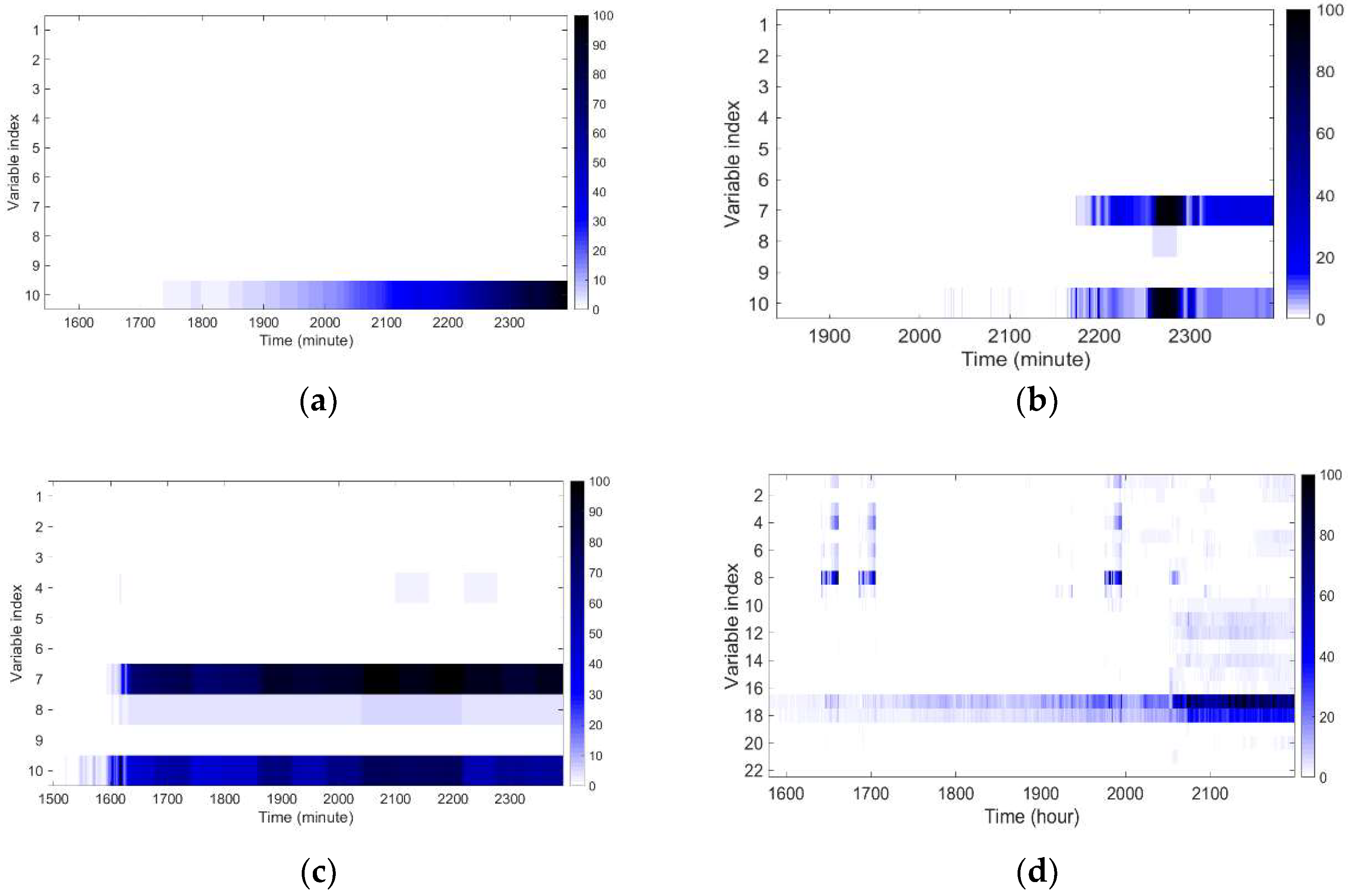
• The development of a CVR-based contribution method for the monitoring of slowly evolving faults. To our best knowledge, it is the first time that it is the first time that CVR-based contribution has been derived and used for fault identification.
• The use of the proposed diagnostic method for incipient fault diagnosis using data captured from a CSTR simulation program and an operational industrial centrifugal compressor.

2. Methods

2.1. CVA-Based Diagnosis

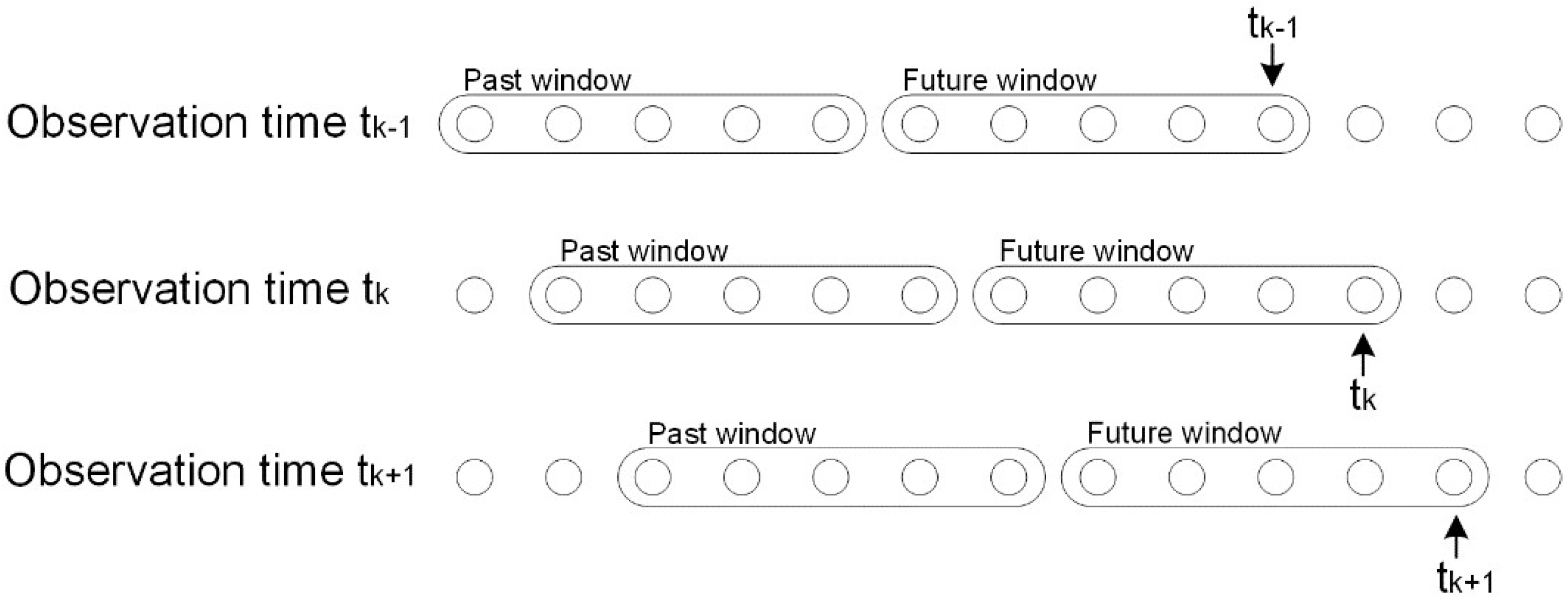
2.1.1. CVA Revisited

$$y_{a,t}=\left[\begin{array}{c}\begin{array}{c}{y}_{t-1}\\ y_{t-2}\end{array}\\ ⋮\\ y_{t-a}\end{array}\right]\in {\mathcal{R}}^{na}$$

(1)

$$y_{b,t}=\left[\begin{array}{c}\begin{array}{c}{y}_t\\ y_{t+1}\end{array}\\ ⋮\\ y_{t+b-1}\end{array}\right]\in {\mathcal{R}}^{nb}$$

(2)

$y_{a,t}$ and $y_{b,t}$ are then normalized to the zero-mean vectors ${\widehat{y}}_{a,t}$ and ${\widehat{y}}_{b,t}$ in order to avoid the domination of variables with excessive values. Then, the normalized future and past vectors ${\widehat{y}}_{a,t}$ and ${\widehat{y}}_{b,t}$ are rearranged as follows:

$${\widehat{Y}}_a=\left[{\widehat{y}}_{a,t+1},{\widehat{y}}_{a,t+2},\dots ,{\widehat{y}}_{a,t+N}\right]\in {\mathcal{R}}^{na\times N}$$

(3)

$${\widehat{Y}}_b=\left[{\widehat{y}}_{b,t+1},{\widehat{y}}_{b,t+2},\dots ,{\widehat{y}}_{b,t+N}\right]\in {\mathcal{R}}^{nb\times N}$$

(4)

in order to generate the reshaped matrices ${\widehat{Y}}_a$ and ${\widehat{Y}}_b$. In Equations (3) and (4), $N=M-a-b+1$ and $M$ denotes the length of $y_t$. Then the covariance matrices of ${\widehat{Y}}_a$ and ${\widehat{Y}}_b$, namely ${\sum }_{a,a}$ and ${\sum }_{b,b}$ as well as the cross-covariance matrix ${\sum }_{a,b}$ can be computed from:

$${\sum }_{a,a}={\widehat{Y}}_a{{\widehat{Y}}_a}^T/\left(N-1\right),{\sum }_{b,b}={\widehat{Y}}_b{{\widehat{Y}}_b}^T/\left(N-1\right),{\sum }_{b,a}={\widehat{Y}}_b{{\widehat{Y}}_a}^T/\left(N-1\right)$$

(5)

The vector of canonical correlations $\sum =diag\left({\lambda }_1,\dots ,{\lambda }_k\right)$, ${\lambda }_1\ge {\lambda }_2\ge \cdots \ge {\lambda }_k>0$ is achieved by performing singular value decomposition (SVD) on the Hankel matrix $\mathcal{H}$:

$$\mathcal{H}={{\sum }_{b,b}}^{-1/2}{\sum }_{b,a}{{\sum }_{a,a}}^{-1/2}=U\sum V^T$$

(6)

Suppose that two data sets ${\widehat{Y}}_a\in {\mathcal{R}}^{na\times N}$ and ${\widehat{Y}}_b\in {\mathcal{R}}^{nb\times N}$ are available for diagnosing possible anomalies. The remaining issue is to compute the diagnostic observers that can achieve satisfactory fault diagnostic performance with a given threshold. In conventional CVA-based approaches, only past data vectors ${\widehat{y}}_{a,t}$ are used to construct test statistics:

$$z_t=K{\widehat{y}}_{a,t}=V_q^T{\sum }_{a,a}^{-1/2}{\widehat{y}}_{a,t}$$

(7)

$$e_t=G{\widehat{y}}_{a,t}=V_{na-q}^T{\sum }_{a,a}^{-1/2}{\widehat{y}}_{a,t}$$

(8)

2.1.2. $T^2$ and $Q$ Indices

Two widely used indices, Hotelling’s $T^2$ and the $Q$ indices [24,25], are computed based on the state and residual space information $z_t$ and $e_t$, respectively.

$$T^2=z_t^T{z}_t$$

(9)

$$Q=e_t^T{e}_t$$

(10)

2.1.3. $T_d$ Index

Motivated by the fact that CVA is able to find maximum correlations between two data sets, practitioners can detect small changes by examining how far away future canonical variates are deviated from past canonical variates (e.g., by examining the usual correlation between past and future). This leads to a diagnostic observer called canonical residuals that quantifies the distinctions between the past and future measurements. Canonical residuals are generated as:

$$r_t=L_q^T{\widehat{y}}_{b,t}-{\sum }_q{J}_q^T{\widehat{y}}_{a,t}$$

(11)

where $L_q^T$ denotes the first $q$ rows of the projection matrix $L^T$, and $L^T={\sum }_{b,b}^{-1/2}{U}_q^T$. Similarly, $J_q^T$ is the first $q$ rows of the projection matrix $J^T$, and $J^T={\sum }_{a,a}^{-1/2}{V}_q^T$. ${\sum }_q=diag\left({\lambda }_1,{\lambda }_2,\dots ,{\lambda }_q\right)$ is a diagonal matrix with its diagonal elements being the first $q$ canonical correlations calculated as Equation (6). Canonical residuals are measures of the discrepancies between the past and future measurements and are able to provide more effective feature representation of small shifts in the early stage of emerging faults compared with diagnostic statistics derived from the traditional CVA approach [26].

Since the condition monitoring data are mean-variance normalized, the mean of the canonical residuals $r_t$ is:

$$E\left(r_t\right)=L_q^{T}E\left({\widehat{y}}_{b,t}\right)-{\sum }_q{J}_q^{T}E\left({\widehat{y}}_{a,t}\right)=0$$

(12)

The covariance of $r_t$ can be calculated as:

$$\begin{array}{c}\hfill {\sum }_r=E\left(r{r}^T\right)=J_q^{T}E\left({\widehat{y}}_{a,t}{{\widehat{y}}_{a,t}}^T\right)J+\sum L_q^{T}E\left({\widehat{y}}_{b,t}{{\widehat{y}}_{b,t}}^T\right)L_q^T{\sum }^T-J_q^{T}E\left({\widehat{y}}_{a,t}{{\widehat{y}}_{b,t}}^T\right)L_q^T{\sum }^T\\ \hfill -\sum L_q^{T}E\left({\widehat{y}}_{b,t}{{\widehat{y}}_{a,t}}^T\right)J=I+\sum {\sum }^T-\sum {\sum }^T-\sum {\sum }^T=I-\sum {\sum }^T\hspace{1em}\end{array}$$

(13)

The distinctions between the past and future measurements are centered around a zero mean under healthy conditions. Hence, diagnostic test statistics can be calculated as the multivariate standard distance of the discrepancy features from zero [27]:

$$\begin{array}{cc}\hfill T_d& =f\left(c{\left(r_t-0\right)}^T{S}^{-1}\left(r_t-0\right)\right)=\frac{\left|c{\left(r_t-0\right)}^T{S}^{-1}\left(r_t-0\right)\right|}{\left|c\right|\left[{\left(r_t-0\right)}^T{S}^{-1}S{S}^{-1}\left(r_t-0\right)\right]}\hfill \\ & ={\left[{\left(r_t\right)}^T{S}^{-1}\left(r_t\right)\right]}^{1/2}={\left[r_t^T\left(I-\sum {\sum }^T\right)r_t\right]}^{1/2}\hfill \end{array}$$

(14)

where $c$ is a normalizing constant, and $S=I-\sum {\sum }^T$ is the covariance matrix of the test and the healthy data. The roots of the multivariate standard distance between two random vectors can be traced back to the results presented in [27], which is described as follows:

Given two random vectors $x_1$ and $x_2$, the univariate standard distance between the two vectors is defined as:

$$f\left(a\right)=\left|a^T{x}_1-a^T{x}_2\right|/{\left(a^{T}Sa\right)}^{1/2}$$

(15)

where $a$ is a vector of unit length and $a^{T}a=1$. $a^T{x}_1$ and $a^T{x}_2$ are the orthogonal projections of the vectors $x_1$ and $x_2$ on the linear space spanned by $a$, respectively. $S$ is the covariance matrix of $x_1$ and $x_2$. Thus, $f\left(a\right)$ denotes the univariate standard distance between vectors $x_1$ and $x_2$ in the one-dimensional subspace spanned by $a$. According to [27], the multivariate standard distance between $x_1$ and $x_2$ is attained for $a=c{\left(x_1-x_2\right)}^T{S}^{-1}\left(x_1-x_2\right)$ and takes the value:

$$T_d=f\left(c{\left(x_1-x_2\right)}^T{S}^{-1}\left(x_1-x_2\right)\right)={\left[{\left(x_1-x_2\right)}^T{S}^{-1}\left(x_1-x_2\right)\right]}^{1/2}$$

(16)

2.1.4. Combined Index $T_c$

In this study, fault detection is carried out using a new health index $T_c$ that combines Hotelling’s $T^2$ and $Q$ statistics and the CVR-based monitoring index $T_d$.

$$T_c=\frac{T^2}{{\sigma }^{T^2}}+\frac{Q}{{\sigma }^Q}+\frac{T_d}{{\sigma }^{T_d}}$$

(17)

where ${\sigma }^{T^2}$, ${\sigma }^Q$ and ${\sigma }^{T_d}$ denote the control limit of $T^2$, $Q$ and $T_d$ index, respectively.

Equation (17) generalizes the combined expression by Alcala and Qin [16] to include $T_d$. Fault detection is implemented by comparing the values of the new monitoring index with a pre-defined threshold. In this study, all control limits are calculated from an adaptive kernel density estimator based on a linear diffusion process [28]. A non-parametric density estimator can provide an estimate of density for any given random data and has been widely applied for fault diagnosis. In the traditional CVA methods, fault thresholds are obtained based on the assumption that the density of the $T^2$, $Q$ and $T_d$ indices are Gaussian, which may not hold true in real-world applications due to the presence of system nonlinearities. Later on, a kernel density estimation method was put forward [24] to solve this problem. However, this method lacks local adaptivity, which may result in high sensitivity to outliers [28]. Moreover, the kernel density estimation method involves a bandwidth selection procedure, which requires a preliminary normal model to be determined. The adaptive kernel density estimator which is used in this study completely avoids the bandwidth selection process and is thus strictly non-parametric and suitable for online monitoring. Furthermore, the adaptive density estimator improves local adaptivity as the estimator is regarded as a transition density of a linear diffusion process. After the probability density functions are estimated from the sample data of the $T^2$, $Q$ or $T_d$ indices, the threshold for individual health indicators is calculated from the probability density function (PDF) for a given significance level $\alpha$ as follows:

$${{\displaystyle \int }}_{-\infty }^{T_{\alpha }^2}p\left(I\right)dI=\alpha$$

(18)

where $I$ denotes indices ${\sigma }^{T^2}$, ${\sigma }^Q$ or ${\sigma }^{T_d}$, $p\left(I\right)$ denotes the PDF of a health indicator, and $T_{\alpha }^2$ is the calculated fault threshold.

The determination of an appropriate fault threshold is crucial because selecting a threshold too large will lead to the index being too insensitive, while selecting a threshold too small will lead to the index being over sensitive to outliers. The adaptive kernel density estimation approach used in this paper is a promising alternative to conventional estimators that involve a bandwidth selection process as the bandwidth is chosen automatically. For a fair comparison with the $T^2$ and $Q$ indices, fault thresholds for $T_d$ are calculated with the same settings as those for $T^2$ and $Q$ indices.

Figure 1 illustrates how the observation window of vectors $\left[y_{a,t},y_{b,t}\right]$ is updated at each sampling time. For the CVR-based online monitoring, each new observation enters the future observation window of length $b$, while the past observation window slides by a single increment in order for updating the samples covered by the past window. The past and future observation window updates recursively as a new measurement becomes available.

2.2. CVA-Based Fault Identification

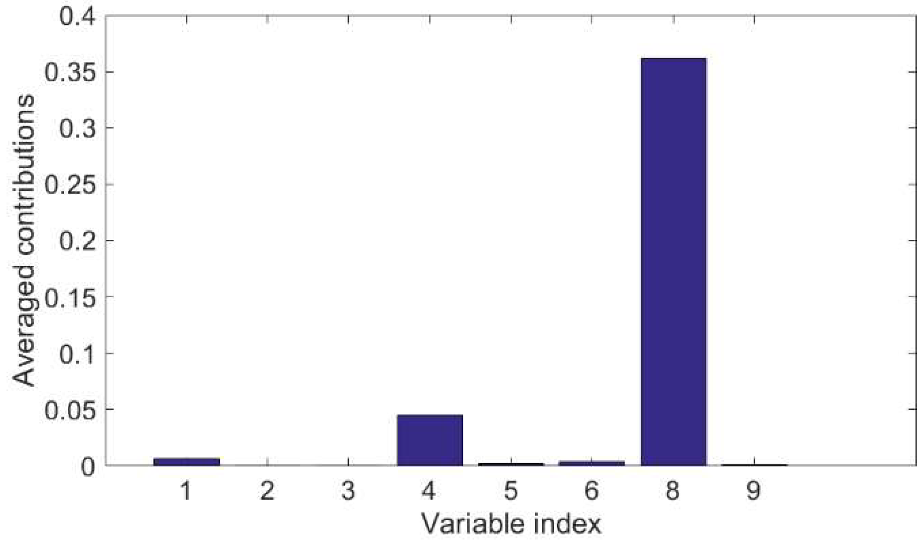
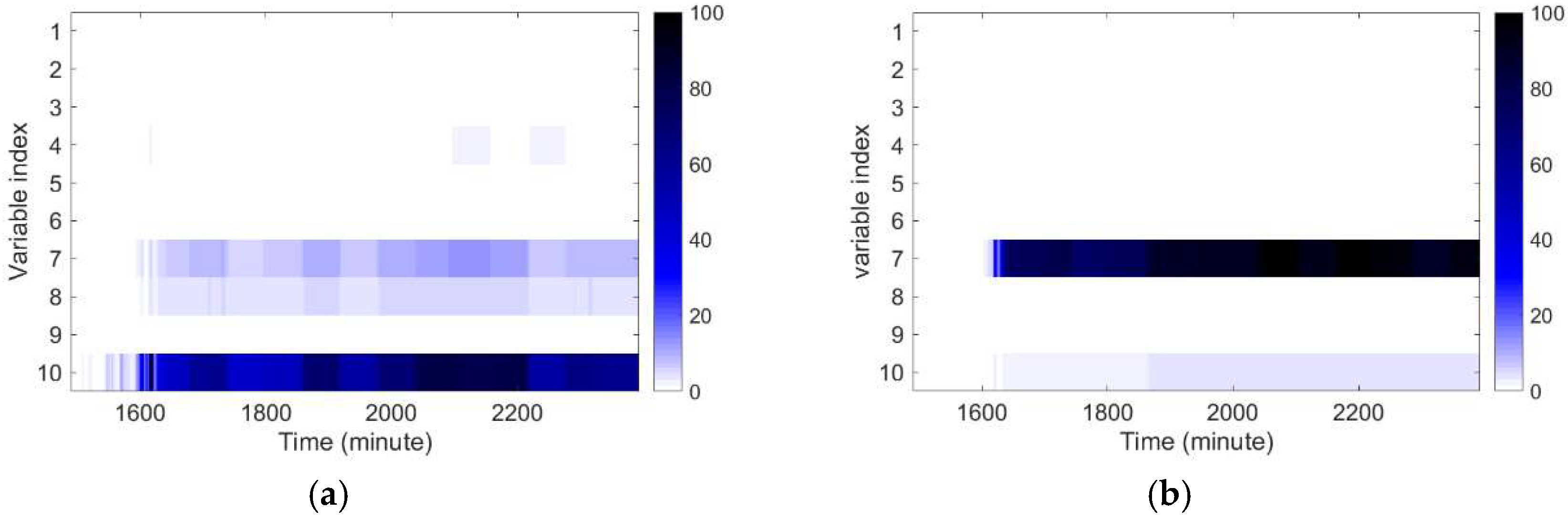
2.2.1. CVA-Based Contributions

The following definition of CVA-based variable contribution was proposed by Jiang et al. [19]:

$$C_{T^2}=T^2=z^{T}z=z^{T}K{\widehat{y}}_{a,t}={\displaystyle \sum }_{i=1}^n{\displaystyle \sum }_{j=1}^q{z}_j{K}_{j,i}{\widehat{y}}_{a,i}={\displaystyle \sum }_{i=1}^n{C}_{i,T^2}$$

(19)

$$C_Q=Q=e^{T}e=e^{T}G{\widehat{y}}_{a,t}={\displaystyle \sum }_{i=1}^n{\displaystyle \sum }_{j=1}^{na-q}{e}_j{G}_{j,i}{\widehat{y}}_{a,i}={\displaystyle \sum }_{i=1}^n{C}_{i,Q}$$

(20)

$$C_{T^2,Q}=0.5C_{T^2}+0.5C_Q$$

(21)

where $C_{T^2}$ and $C_Q$ denote the variable contribution (or fault score) calculated based on the state and residual space information in the CVA model, respectively. $C_{i,T^2}$ is the contribution of variable ${\widehat{y}}_i$ to the monitoring statistic $T^2$ and $C_{i,Q}$ is the contribution of ${\widehat{y}}_i$ to the monitoring statistic $Q$. $z_j{K}_{j,i}{\widehat{y}}_{a,i}$ is the contribution of variable ${\widehat{y}}_i$ to the $j$th canonical variate $z_j$. Similarly, $e_j{G}_{j,i}{\widehat{y}}_{a,i}$ denotes the contribution of variable ${\widehat{y}}_i$ to the $j$th canonical residual variate $e_j$. The combined contribution according to [19] uses equal weights for the state and residual space contribution $C_{T^2,Q}=0.5C_{T^2}+0.5C_Q$.

The proposed CVR-based contribution is calculated as follows:

$$C_{T_d}={r_t}^T{\left(I-{-}_q^2\right)}^{-1}{r}_t={\displaystyle \sum }_{i=1}^n{\displaystyle \sum }_{j=1}^q{r}_j{{\sum }_{dd}^{-1}}_j\left(L_{j,i}{\widehat{y}}_{b,i}-{-}_j{J}_{j,i}{\widehat{y}}_{a,i}\right)={\displaystyle \sum }_{j=1}^n{C}_{i,T_d}$$

(22)

where ${\sum }_{dd}^{-1}={\left(I-{-}_q^2\right)}^{-1}$, and $C_{T_d}{\sum }_{dd}^{-1}={\left(I-{-}_q^2\right)}^{-1}$ denotes the state space contribution.

$$C_{T_d,Q}=0.5C_{T_d}+0.5C_Q$$

(23)

where $C_Q$ is the residual space contribution, and $C_{T_d,Q}$ denotes the proposed CVR-based combined contribution.

3. Results

3.1. Fault Description

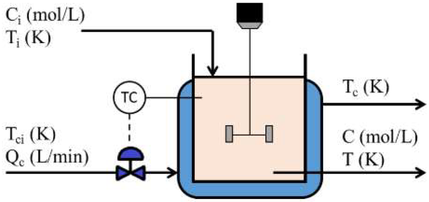
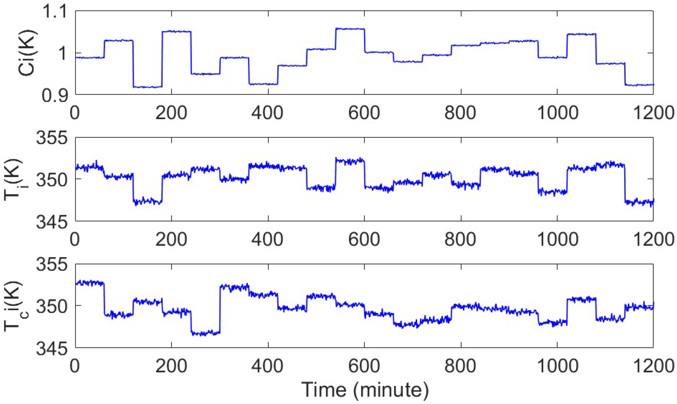
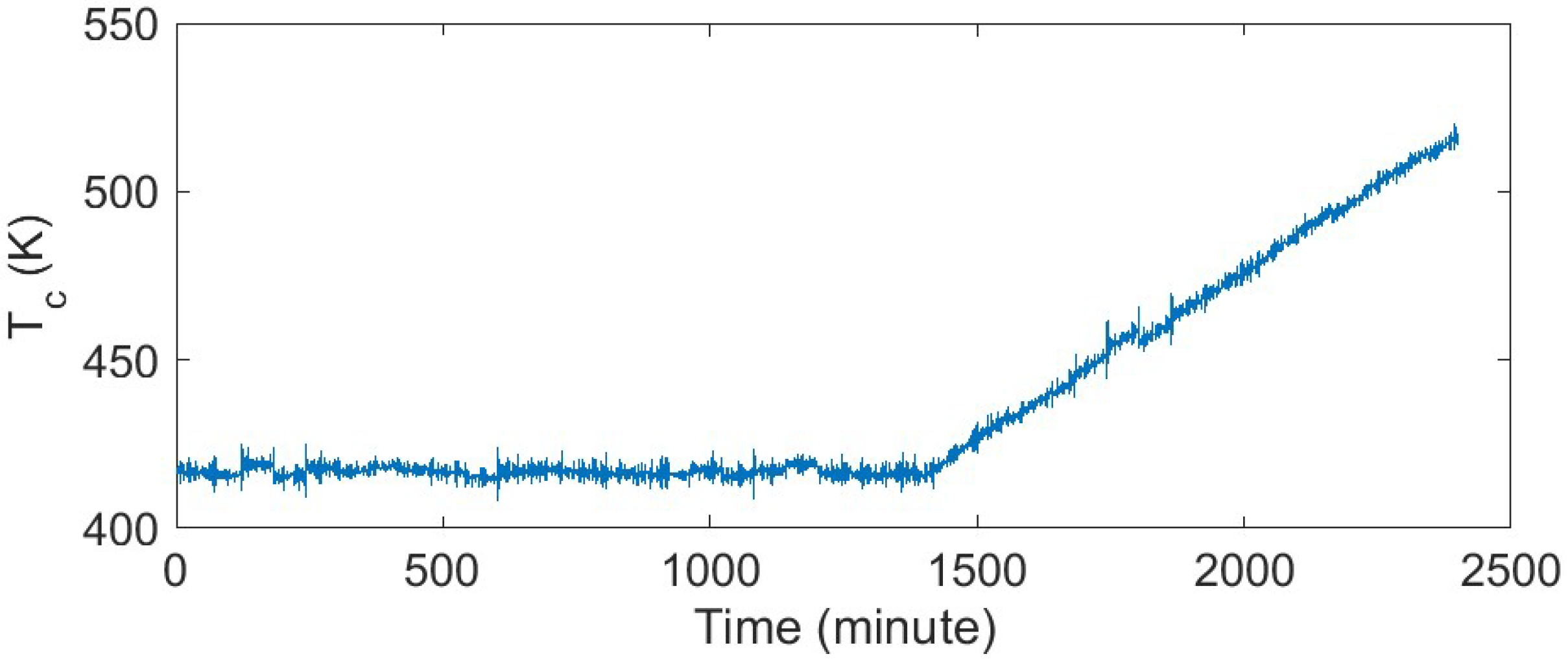
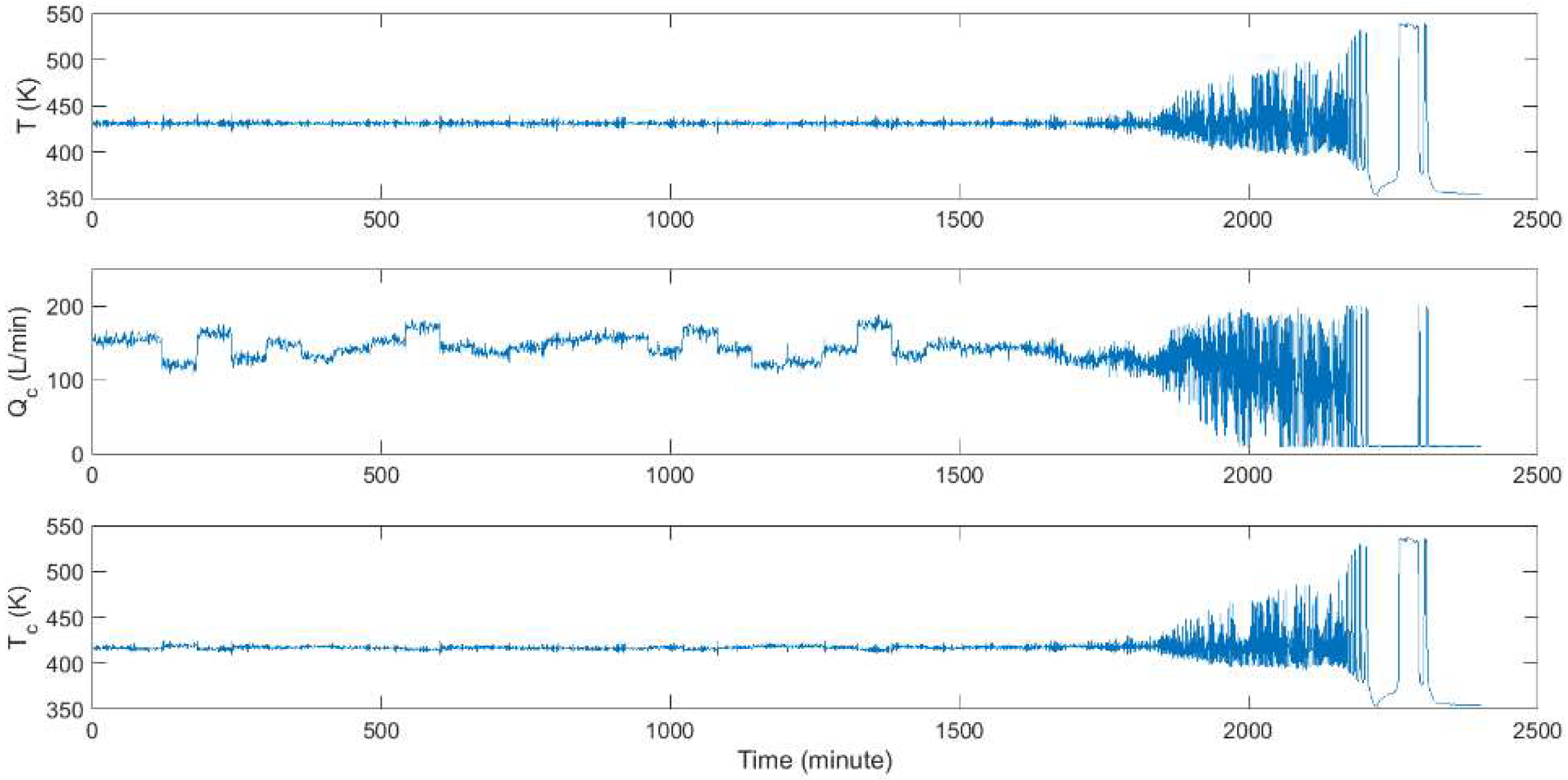
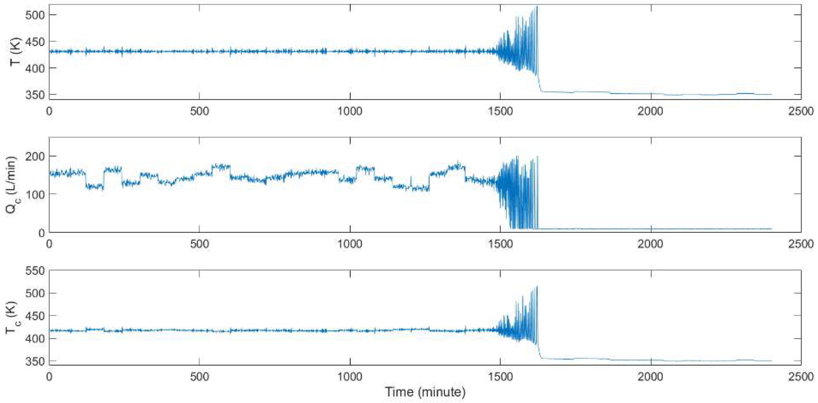
3.1.1. CSTR Fault Description

The proposed method is first evaluated using data created from a CSTR system. The CSTR Simulink model utilized in this study was generated by the authors of [14], which was designed especially for simulating incipient faults. The CSTR model is simulated using Matlab Simulink.

Table 1. Slowly evolving fault scenarios in the continuous stirred tank reactor (CSTR) system.

Fault ID	Fault Description	Decaying rate	Fault Type
1	$T_c=T_{c,0}+\alpha t$	$\alpha =0.1$	Additive
2	$a_1=a_0\exp \left(-\alpha t\right)$	$\alpha =0.0006$	Multiplicative
3	$a_1=a_0\exp \left(-\alpha t\right)$	$\alpha =0.003$.	Multiplicative

summarizes the process variables for this CSTR system. Among these variables, the system inputs are $C_i$, $T_i$ and $T_{ci}$, and the system outputs are $C$, $T$, $T_c$ and $Q_c$. The schematic of the CSTR is shown in Figure 2. A detailed description of the process can be found in [14]. The CSTR process’ dynamic model is formulated as:

$$\frac{dC}{dt}=\frac{Q}{V}\left(C_i-C\right)-a_{1}kC+v_1$$

(24)

$$\frac{dT}{dt}=\frac{Q}{V}\left(T_i-T\right)-a_1\frac{\left(\Delta H_r\right)kC}{\rho C_{p}V}\left(T-T_c\right)+v_2$$

(25)

$$\frac{d{T}_c}{dt}=\frac{Q_c}{V_c}\left(T_{ci}-T_c\right)+b_1\frac{UA}{{\rho }_C{C}_{pc}{V}_c}\left(T-T_c\right)+v_3$$

(26)

where $Q$ is inlet flow rate, $\Delta H_r$ represents heat of reaction, $UA$ is the heat transfer coefficient, $\rho$ and ${\rho }_C$ are fluid density, $C_p$ and $C_{pc}$ are fluid heat capacity, and $V$ and $V_c$ are tank and jacket volume, respectively.

Healthy and unhealthy data sets were obtained from the CSTR model for 1200 min of operation. All data were obtained at a sampling rate of one sample per minute. As shown in Figure 3, the operating conditions were deliberately varied by perturbing the system inputs around their mean values every sixty samples. For faulty data sets, each testing dataset started with no fault, and the fault starts after 200 min of operation. The name of different process variables is summarized in Table 1.

Three fault scenarios were utilized to assess the effectiveness of the proposed fault detection approach. The different types of faulty conditions considered are summarized in Table 1. The parameter $a_1$ was set to one during normal operating conditions. During faulty conditions, $a_1$ decayed gradually from one toward zero. All faults were introduced after 1400 min of normal operation. The faulty variables sample dataset for fault 1, 2, and 3 are shown in Figure 4, Figure 5 and Figure 6. It is worth noting that fault 2 and fault 3 become visible at different times because the decaying rates were deliberately varied. Measured variables of the CSTR process are summarized in

Table 2. Measured variables of CSTR process.

Variable ID	Variable	Units
1	$C_i$ (noise-free)	mol/L
2	$T_i$ (noise-free)	K
3	$T_{ci}$ (noise-free)	K
4	$C_i$	mol/L
5	$T_i$	K
6	$C$	mol/L
7	$T$	K
8	$T_c$	K
9	$T_{ci}$	K
10	$Q_c$	L/min

.

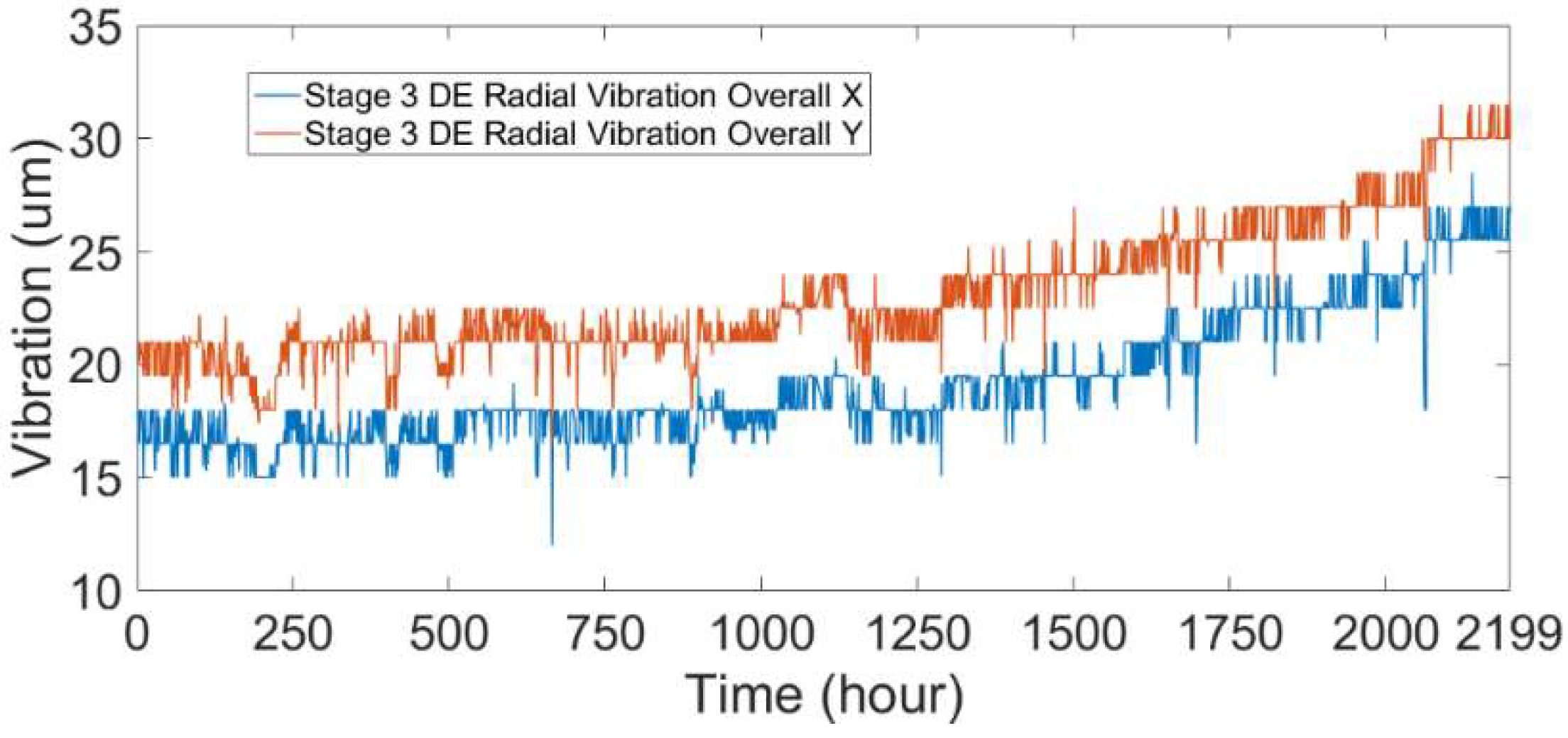
3.1.2. Compressor Fault Description

In order to further assess the ability of the proposed diagnostic technique to effectively detect incipient faults and identify faulty variables, the model was tested using data captured from an operational industrial compressor. This machine is a high-pressure centrifugal compressor running at a large refinery in Europe (hereafter referred to as compressor A). The measured time series from compressor A consisted of 2199 observations and 22 variables.

Table 3. Measured variables of compressor A.

ID	Variable Name	ID	Variable Name
1	Stage 1 Suction Pressure	12	Stage 1–2 DE Radial Vibration Overall Y *
2	Stage 1 Discharge Pressure	13	Stage 1–2 NDE Radial Vibration Overall X *
3	Stage 1 Suction Temperature	14	Stage 1–2 NDE Radial Vibration Overall Y *
4	Stage 1 Discharge Temperature	15	Stage 1–2 Thrust Position Axial Probe 1
5	Stage 2 Suction Pressure	16	Stage 1–2 Thrust Position Axial Probe 2
6	Stage 2 Discharge Pressure	17	Stage 3 DE Radial Vibration Overall X *
7	Stage 2 Suction Temperature	18	Stage 3 DE Radial Vibration Overall Y *
8	Stage 2 Discharge Temperature	19	Stage 3 NDE Radial Vibration Overall X *
9	Stage 3 Suction Pressure	20	Stage 3 NDE Radial Vibration Overall Y *
10	Stage 3 Discharge Pressure	21	Stage 3 Thrust Position Axial Probe 1
11	Stage 1–2 DE Radial Vibration Overall X *	22	Stage 3 Thrust Position Axial Probe 2

* DE is short for drive end, and NDE is short for non-drive end.

summarizes the names of different process variables. For this study, all data were captured at a sampling rate of one sample per hour. As shown in Figure 7, the root-cause variables are the two different bearing–vibration sensors; the machine continued to run until the 2199th sampling point.

3.2. Fault Detection

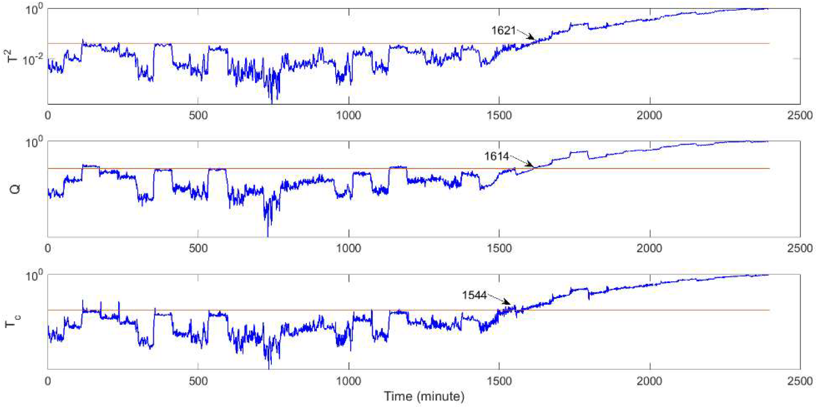
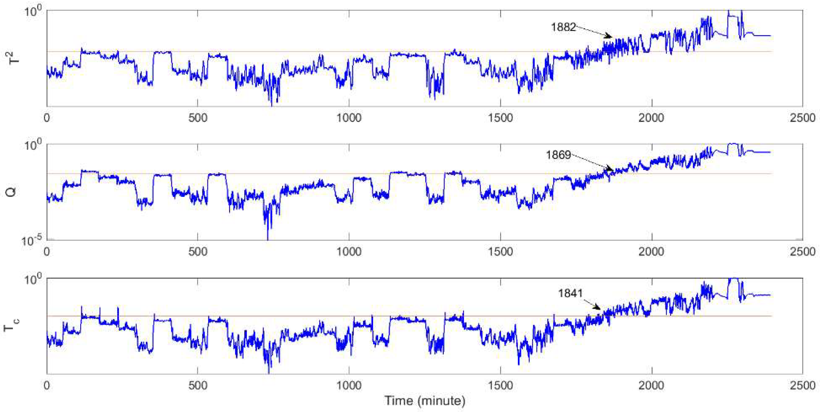
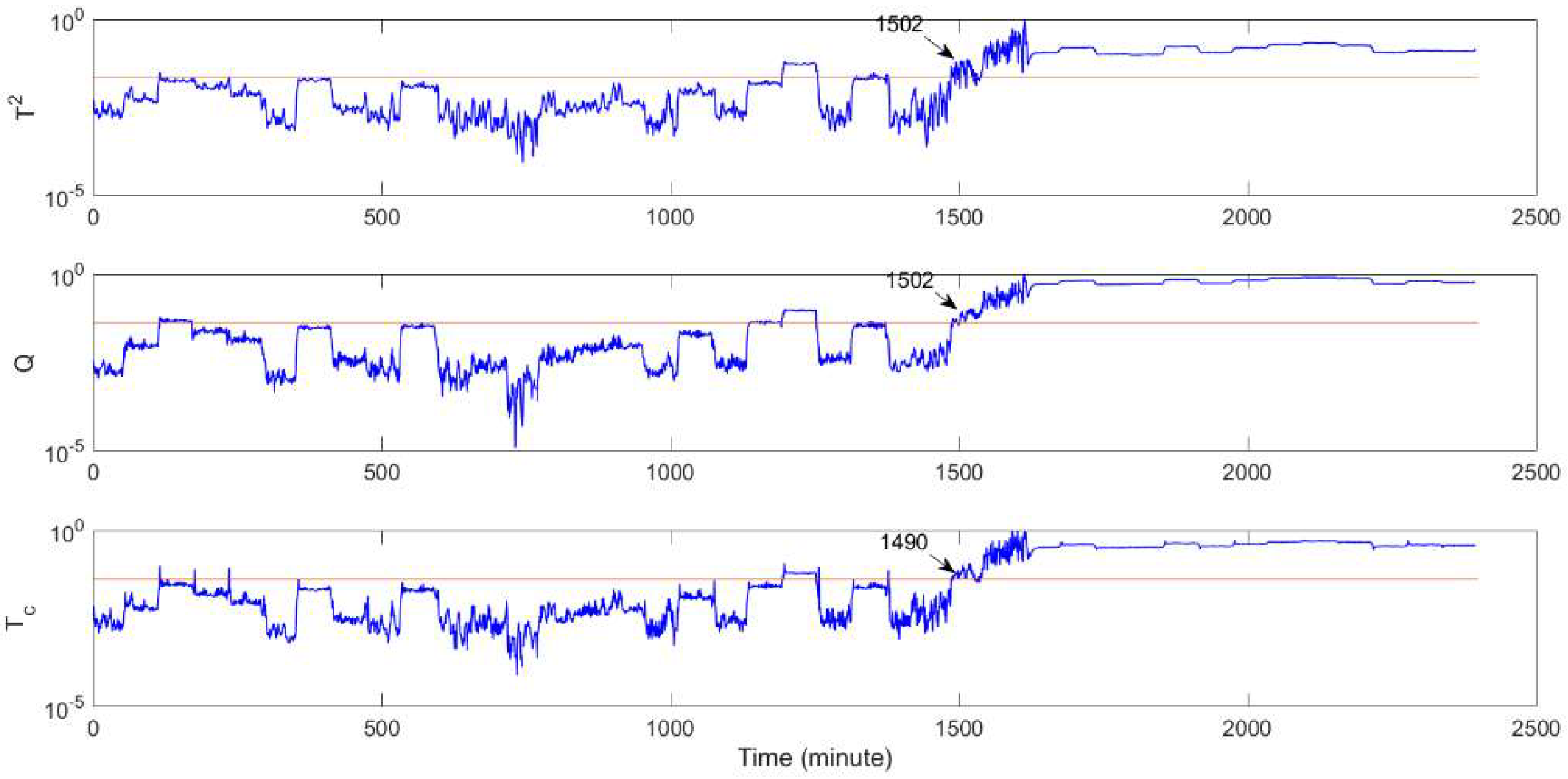
3.2.1. CSTR Fault Detection

The CVR-based diagnostic approach is first trained using a data set collected from normal operating conditions. The scale of time lags $a$ and $b$ were estimated through the autocorrelation analysis [5] of the root summed squares of all variables in the training data set. Here the number of time lags $a$ and $b$ were set to five. Since the underlying process data is non-stationary and non-linear, and does not follow a Gaussian distribution, a kernel density estimator based on a linear diffusion process [28] was adopted here to determine the upper control limits of the test statistics. All upper control limits for healthy operational conditions in this investigation were calculated at the 99% confidence level (i.e., the probability the test statistics are smaller than the predefined threshold is 99%). A key step in CVA is to determine the order of the reduction, that is, its number of retained states $q$. In this study, the optimal number of retained states $q$ was selected such that the false alarm rate is minimized during cross-validation. For the purpose of finding the optimal number of $q$ which gives the lowest false alarm rate, a healthy dataset containing 1200 observations was used to test the trained CVA diagnostic model. The false alarm rate was plotted against different values of $q$ in Figure 8. For low and high values of dimensionality, the false alarm rate is high due to large number of $T_c$ threshold violations. $q=15$ was finally adopted in this work as it resulted in the lowest number of false positives.

The fault detection results are depicted in Figure 9, Figure 10 and Figure 11. Two performance metrics: (1) detection time (DT) and (2) missed detection rate (MDR) are utilized to evaluate the performance of the proposed $T_c$ index and its counterparts. MDR is computed as:

$$MDR=\frac{\sum samples \left(I<I_{threshold}|fault\right)}{total no. of samples}$$

(27)

where $I$ denotes a monitoring index and $I_{threshold}$ denotes the corresponding upper control limit.

It is visible from Figure 9 that the combined index detects the fault at 1544 min of sampling time, providing ample time to plan maintenance activities, while $T^2$ and $Q$ become sensitive to the fault only after 1614 min of sampling time. In Figure 10 and Figure 11, both $T^2$ and $Q$ struggle to cross the fault threshold, leading to a higher MDR (see

Table 4. Monitoring results for the CSTR and pump faults.

Fault Type		${\mathit{T}}^2$	$\mathit{Q}$	${\mathit{T}}_{\mathit{c}}$
CSTR fault 1	Detection time (min)	1626	1619	1544
	Missed detection rate (%)	8.75%	9.04%	6.5%
CSTR fault 2	Detection time (min)	1882	1869	1841
	Missed detection rate (%)	20.08%	19.29%	18.42%
CSTR fault 3	Detection time (min)	1502	1502	1490
	Missed detection rate (%)	4.37%	4.17%	4.04%
Compressor	Detection time (min)	1641	1976	1579
	Missed detection rate (%)	2.82%	19.37%	0.55%

), while $T_c$ appears to be more sensitive to small changes at the initial stage of the fault. Table 4 summarizes the performance of the fault detection methods studied. The bold values show the fault cases where CVR presents a superior performance than $T^2$ and $Q$ statistics. It is observed that the combined index $T_c$ is more sensitive than $T^2$ and $Q$ for slowly developing faults, leading to earlier fault detection times. Also, the $T_c$ index resulted in lower missed detections than the other two statistics under faulty operating conditions, thereby making it a promising alternative to existing indices.

As mentioned previously, the performance of CVA is superior to other dimension reduction techniques when validated using a multiphase flow facility [3] working under changing operating conditions. The proposed diagnostic method inherits the strength of CVA in handling varying operating conditions, leading to low false alarm rates for all the faulty cases studied (see

Table 5. False alarm rate of $T_c$ index.

Fault Type	CSTR Fault 1	CSTR Fault 2	CSTR Fault 3	Compressor
False alarm rate	1.13%	0.71%	2.76%	3.25%

).

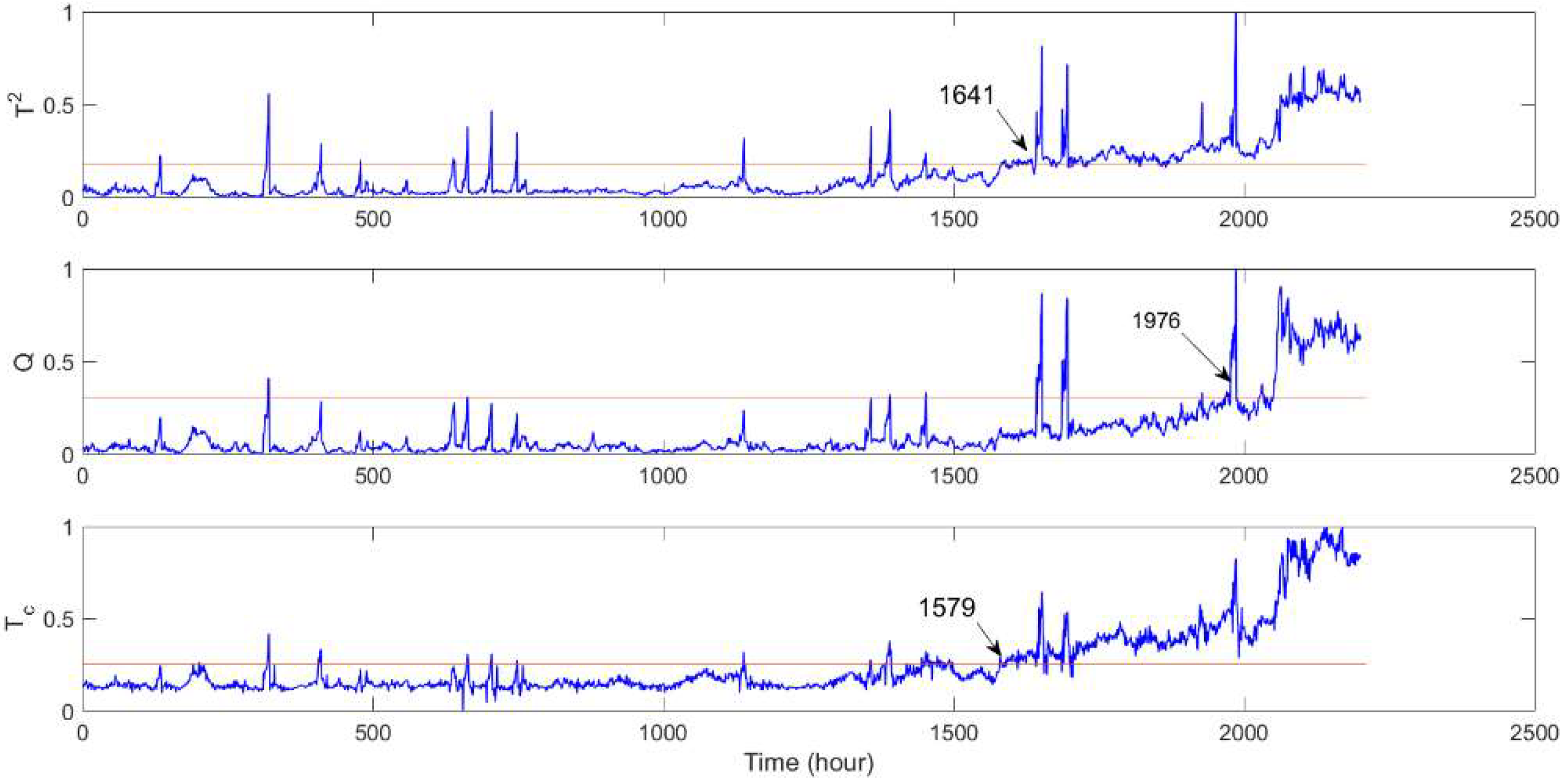
3.2.2. Compressor Fault Detection

Similar to the procedure described in Section 3.2.1, the scale of time lags $a$ and $b$ were estimated through the autocorrelation analysis and were both set to 10 in this study. The optimal number of retained states $q$ in the CVA model was estimated by inspecting the false alarm rate against different number of retained states. According to the results shown in Figure 12, the number of $q$ was set to 17 in the CVA diagnostic model. Figure 13 shows the results obtained in terms of fault detection. The combined monitoring index $T_c$ is able to distinguish normal operating conditions from real faults incurring dynamics anomalies and thereby results in the early detection of faults with a short time delay. In this case, $T^2$ struggles to cross the threshold between 1641 min samples and 1579 min samples, leading to a high MDR as shown in Table 4. The $Q$ statistic, however, is insensitive to the fault and can only detect the fault at the late stage of degradation. The fault detection time and missed detection rate for different indices are demonstrated in Table 4.

3.3. Fault Identification

After fault detection, the proposed CVR-based method is applied to identify the influential variables associated with the detected faults. The resultant contribution plots for the CSTR and compressor fault cases are depicted in Figure 14. In each contribution plot, the sampling time denotes the horizontal axis and the variable index denotes the vertical axis. The stronger the contribution of a variable is, the larger the fault-related deviations associated with the specific variable is. At each faulty condition, faulty variables will show continuously strong bands of contribution after the fault is detected by the combined health index.

CSTR fault case 1 simulates sensor drifts on the measured variable $T_c$, and thus variable 10 is the only fault influential variable. Fault 2 and fault 3, however, simulate catalyst decay at different decaying rates; therefore the associated faulty variables are variables 7, 8 and 10. It is observed in Figure 14a that the contributions of variable 10 are higher than the normal variables for the CVR-based contribution, indicating that variable 10 is successfully identified as the faulty variable for fault 1. Based on the information provided by the CVR-based contributions for CSTR fault case 2, variables 7 and 10 show continuously strong bands of contribution throughout the degradation process, making them distinct from fault-free variables. Although variable 8 only demonstrates large contributions at around 2260–2280 min samples in Figure 14b, its contribution is still much higher on average over all faulty samples than the normal variables (see Figure 15; the fault scores of variable 8 are much higher than those of variables 1–6 and 9). Further investigation is required into the process so as to verify the observations.

It is observed in Figure 14c that variables 7, 8 and 10 are successfully identified as faulty variables because of their continuously strong contributions throughout the deterioration process. State space and residual space contribution plots for CSTR fault 3 are also shown in Figure 16a,b, respectively. Most faulty variables (except variable 8) are identified through Figure 16b, with variable 7 being the most influential variable. Figure 16a identifies all faulty variables, with variable 10 being the most influential variable. The combined contribution plot shown in Figure 14c identifies all faulty variables and enhances the contributions from variable 7, leading to a more accurate contribution map for CSTR fault 3. This observation highlights the advantages of the combined contribution plot in identifying influential variables compared with state space/residual space contribution map. State space contributions are calculated using the canonical residuals $r_t$ and the first $q$ canonical correlations ${\sum }_q$ as per Equation (22), while residual space contributions are calculated based on the last $na-q$ columns of $V$ as per Equation (20). Influential variables identified in the state space are associated with the large deviations of the states that present during healthy operational conditions. The residual space contributions, however, are related to the new states which are not described by the healthy CVR model. It is observed from Figure 14d that the influential variables are stage 3 drive end (DE) vibration sensors, which agrees with the time-domain observations.

4. Conclusions

The CVR-based diagnostic method proposed in this paper extended the concept of CVA in fault detection and identification of abrupt faults to the situation of diagnosis of slowly involving faults. The consideration of canonical variate residuals resulted in a more sensitive monitoring index compared with $T^2$ and $Q$ statistics. When validated on simulation and industrial case studies, our proposed $T_c$ index outperformed $T^2$ and $Q$ statistics in terms of both fault detection time and missed detection rate. Moreover, by considering the deviations between past and future data in the canonical state space, the proposed CVR-based contribution plots successfully identified faulty variables for most of the fault cases studied. The importance of the combination of state and residual space contributions was also highlighted.

The CVR-based contribution method appeared to be less sensitive to small changes in the data because it tends to give low fault scores during the early degradation process. A consideration for future study is whether the fault scores at early degradation stages would be improved if deviations between past and future data in the residual space were used for the identification of faulty variables. The removal of the smearing effect caused by normal variables is also a future research direction. The challenge of using CVR for fault detection can be the change of the operating conditions, which are not easily discriminated from failures even though the overall false alarm rate is low. In the future, we will explore approaches that can distinguish between the change of operational conditions and system failures.

References

1. Li, X.; Duan, F.; Mba, D.; Bennett, I. Multidimensional prognostics for rotating machinery: A review. Adv. Mech. Eng. 2017, 9, 1–20. [Google Scholar] [CrossRef]
2. Zhao, R.; Wang, D.; Yan, R.; Mao, K.; Shen, F.; Wang, J. Machine Health Monitoring Using Local Feature-Based Gated Recurrent Unit Networks. IEEE Trans. Ind. Electron. 2018, 65, 1539–1548. [Google Scholar] [CrossRef]
3. Wook, S.; Lee, C.; Lee, J.; Hyun, J.; Lee, I. Fault detection and identification of nonlinear processes based on kernel PCA. Chemom. Intell. Lab. Syst. 2005, 75, 55–67. [Google Scholar]
4. Fan, J.; Wang, Y. Fault detection and diagnosis of non-linear non-Gaussian dynamic processes using kernel dynamic independent component analysis. Inf. Sci. 2014, 259, 369–379. [Google Scholar] [CrossRef]
5. Li, X.; Duan, F.; Loukopoulos, P.; Bennett, I.; Mba, D. Canonical variable analysis and long short-term memory for fault diagnosis and performance estimation of a centrifugal compressor. Control Eng. Pract. 2018, 72, 177–191. [Google Scholar] [CrossRef]
6. Li, W.; Qin, S.J. Consistent dynamic PCA based on errors-in-variables subspace identification. J. Process Control 2001, 11, 661–678. [Google Scholar] [CrossRef]
7. Yin, S.; Zhu, X.; Member, S.; Kaynak, O. Improved PLS Focused on Key-Performance- Indicator-Related Fault Diagnosis. IEEE Trans. Ind. Electron. 2015, 62, 1651–1658. [Google Scholar] [CrossRef]
8. Ruiz-cárcel, C.; Cao, Y.; Mba, D.; Lao, L.; Samuel, R.T. Statistical process monitoring of a multiphase flow facility. Control Eng. Pract. 2015, 42, 74–88. [Google Scholar] [CrossRef] [Green Version]
9. Stefatos, G.; Hamza, A.B. Dynamic independent component analysis approach for fault detection and diagnosis. Expert Syst. Appl. 2010, 37, 8606–8617. [Google Scholar] [CrossRef]
10. Jiang, Q.; Ding, S.X.; Wang, Y.; Yan, X. Data-Driven Distributed Local Fault Detection for Large-Scale Processes Based on the GA-Regularized Canonical Correlation Analysis. IEEE Trans. Ind. Electron. 2017, 64, 8148–8157. [Google Scholar] [CrossRef]
11. Chen, Z.; Ding, S.X.; Peng, T.; Yang, C.; Gui, W. Fault Detection for Non-Gaussian Processes Using Generalized Canonical Correlation Analysis and Randomized Algorithms. IEEE Trans. Ind. Electron. 2018, 65, 1559–1567. [Google Scholar] [CrossRef]
12. Chen, Z.; Zhang, K.; Ding, S.X.; Shardt, Y.A.W.; Hu, Z. Improved canonical correlation analysis-based fault detection methods for industrial processes. J. Process Control 2016, 41, 26–34. [Google Scholar] [CrossRef]
13. Jiang, Q.; Gao, F.; Yi, H.; Yan, X. Multivariate Statistical Monitoring of Key Operation Units of Batch Processes Based on Time-Slice CCA. IEEE Trans. Control Syst. Technol. 2018, 99, 1–8. [Google Scholar] [CrossRef]
14. Pilario, K.E.S.; Cao, Y. Canonical Variate Dissimilarity Analysis for Process Incipient Fault Detection. IEEE Trans. Ind. Inform. 2018, 14, 5308–5315. [Google Scholar] [CrossRef]
15. Samuel, R.T.; Cao, Y. Kernel Canonical Variate Analysis for Nonlinear Dynamic Process Monitoring. IFAC-PapersOnLine 2015, 48, 605–610. [Google Scholar] [CrossRef]
16. Alcala, C.F.; Qin, S.J. Reconstruction-based contribution for process monitoring. Automatica 2009, 45, 1593–1600. [Google Scholar] [CrossRef]
17. Tan, R.; Cao, Y. Deviation Contribution Plots of Multivariate Statistics. IEEE Trans. Ind. Inform. 2019, 15, 833–841. [Google Scholar] [CrossRef]
18. Zhu, X.; Braatz, R.D. Two-Dimensional Contribution Map for Fault Identification. IEEE Control Syst. Mag. 2014, 34, 72–77. [Google Scholar]
19. Jiang, B.; Huang, D.; Zhu, X.; Yang, F.; Braatz, R.D. Canonical variate analysis-based contributions for fault identification. J. Process Control 2015, 26, 17–25. [Google Scholar] [CrossRef]
20. Li, X.; Duan, F.; Mba, D.; Bennett, I. Combining Canonical Variate Analysis, Probability Approach and Support Vector Regression for Failure Time Prediction. J. Intell. Fuzzy Syst. 2018, 34, 746–752. [Google Scholar]
21. Jiang, B.; Braatz, R.D. Fault detection of process correlation structure using canonical variate analysis-based correlation features. J. Process Control 2017, 58, 131–138. [Google Scholar] [CrossRef]
22. Jiang, B.; Zhu, X.; Huang, D.; Paulson, J.A.; Braatz, R.D. A combined canonical variate analysis and Fisher discriminant analysis (CVA–FDA) approach for fault diagnosis. Comput. Chem. Eng. 2015, 77, 1–9. [Google Scholar] [CrossRef]
23. Lu, Q.; Jiang, B.; Gopaluni, R.B.; Loewen, P.D.; Braatz, R.D. Locality preserving discriminative canonical variate analysis for fault diagnosis. Comput. Chem. Eng. 2018, 117, 309–319. [Google Scholar] [CrossRef]
24. Odiowei, P.E.P.; Yi, C. Nonlinear Dynamic Process Monitoring Using Canonical Variate Analysis and Kernel Density Estimations. IEEE Trans. Ind. Inform. 2010, 6, 36–45. [Google Scholar] [CrossRef] [Green Version]
25. Hotelling, H. New Light on the Correlation Coefficient and its Transforms. J. R. Stat. Soc. Ser. B 1953, 15, 193–232. [Google Scholar] [CrossRef]
26. Juricek, B.C.; Seborg, D.E.; Larimore, W.E. Fault Detection Using Canonical Variate Analysis. Ind. Eng. Chem. Res. 2004, 43, 458–474. [Google Scholar] [CrossRef]
27. Flury, B.K.; Riedwyl, H. Standard distance in univariate and multivariate analysis. Am. Stat. 1986, 40, 249–251. [Google Scholar]
28. Botev, B.Z.I.; Grotowski, J.F.; Kroese, D.P. Kernel density estimation via diffusion. Ann. Stat. 2010, 38, 2916–2957. [Google Scholar] [CrossRef] [Green Version]
Figure 1. Illustration of how the future and past windows are updated when a new measurement becomes available.
Energies 12 00726 g001
Figure 2. Schematic of the continuous stirred tank reactor (CSTR) process [14]. T c is the inlet temperature of the cooling water; T c i is the outlet temperature of the i th cooling water; Q c is the coolant flow rate; T i is the temperature of the i th reactor; T is the reactor temperature; Q c is the coolant flow rate; C i is the concentration in the reactor.
Energies 12 00726 g002
Figure 3. Sample dataset (healthy) of system inputs from CSTR simulation.
Energies 12 00726 g003
Figure 4. Sample dataset of faulty variables from CSTR simulation (fault case 1).
Energies 12 00726 g004
Figure 5. Sample dataset of faulty variables from CSTR simulation (fault case 2).
Energies 12 00726 g005
Figure 6. Sample dataset of faulty variables from CSTR simulation (fault case 3).
Energies 12 00726 g006
Figure 7. Trend of two different bearing vibration sensor measurements of compressor A. DE is short for drive end.
Energies 12 00726 g007
Figure 8. False alarm rate for different number of retained states q .
Energies 12 00726 g008
Figure 9. Fault detection results for fault case 1: T 2 (upper), Q (middle) and combined index T c (lower).
Energies 12 00726 g009
Figure 10. Fault detection results for fault case 2: T 2 (upper), Q (middle) and combined index T c (lower).
Energies 12 00726 g010
Figure 11. Fault detection results for fault case 3: T 2 (upper), Q (middle) and combined index T c (lower).
Energies 12 00726 g011
Figure 12. False alarm rate for different number of retained states q .
Energies 12 00726 g012
Figure 13. Fault detection results for compressor fault: T 2 (upper), Q (middle) and combined index T c (lower).
Energies 12 00726 g013
Figure 14. Fault identification results for (a) CSTR fault 1; (b) CSTR fault 2; (c) CSTR fault 3; (d) compressor fault.
Energies 12 00726 g014
Figure 15. Averaged individual variable contributions under faulty conditions from CSTR fault 2.
Energies 12 00726 g015
Figure 16. Contribution plots based on (a) state space information and (b) residual space information for CSTR fault 3.
Energies 12 00726 g016