Appliance Classification by Power Signal Analysis Based on Multi-Feature Combination Multi-Layer LSTM

Abstract

The imbalance of power supply and demand is an important problem to solve in power industry and Non Intrusive Load Monitoring (NILM) is one of the representative technologies for power demand management. The most critical factor to the NILM is the performance of the classifier among the last steps of the overall NILM operation, and therefore improving the performance of the NILM classifier is an important issue. This paper proposes a new architecture based on the RNN to overcome the limitations of existing classification algorithms and to improve the performance of the NILM classifier. The proposed model, called Multi-Feature Combination Multi-Layer Long Short-Term Memory (MFC-ML-LSTM), adapts various feature extraction techniques that are commonly used for audio signal processing to power signals. It uses Multi-Feature Combination (MFC) for generating the modified input data for improving the classification performance and adopts Multi-Layer LSTM (ML-LSTM) network as the classification model for further improvements. Experimental results show that the proposed method achieves the accuracy and the F1-score for appliance classification with the ranges of 95–100% and 84–100% that are superior to the existing methods based on the Gated Recurrent Unit (GRU) or a single-layer LSTM.

1. Introduction

Power consumption in homes and buildings has been dramatically increasing because more and more appliances are being used, and the number of them is also expected to increase. Due to the limited power supply and the constraints on building more power plants, the imbalance of power supply and demand has become an important problem to address. In the past, this issue has been addressed as supply-oriented management whereas it is addressed as power demand management nowadays. For power demand management, it is important to monitor power consumption and adjust power consumption accordingly by notifying the user of any appliances drawing unnecessary power or shift their usage when the power demand is lower. Non-Intrusive Load Monitoring (NILM) [1,2], which is a process that infers the power consumption and monitors the appliances being used from analyzing the aggregated power data without directly measuring through additional hardware, is suitable for this task. In this regard, it has been investigated by many studies [3,4,5]. To monitor an appliance, the power data of each appliance should be classified from the aggregated power data. To do so, the characteristics of the power data of each appliance should be known a priori to the NILM system. So this problem becomes a proper subject for machine learning in a supervised way with an appropriate power dataset.

The power signal carries information of inherent physical characteristics of the appliance along with other characteristics caused by external factors such as environment where the appliance is in operation. The physical characteristics are determined by the internal device configurations that can determine the magnitude, phase, and frequency of the power patterns of the appliance. External factors that change the power characteristics include the supply voltage, external disturbances and appliance usage patterns of the users such as use time, frequency, time duration, etc. These characteristics are important information for appliance classification.

In order to improve the performance of the NILM, it is important to blindly determine which appliances are in operation using the aggregated power data. This requires classification of multiple unknown number of appliances, so-called multi-label classification, from the aggregated power measurement. Because the classifier is typically configured among the last steps of the overall NILM operation [6], the outcome of the classifier can greatly affect the final result of the system. Therefore, algorithms for multi-label classification need to analyze the power characteristic pattern of each appliance effectively and identify the appliances with high accuracy. So, researchers have conducted many studies to improve the classification performance for power data. Various classification algorithms such as Support Vector Machine (SVM) [7,8,9,10,11], k-Nearest Neighbor (k-NN) algorithm [9,10,11,12,13] and Hidden Markov Model (HMM) [11,14,15,16,17,18]—which is a sequential approach—have been proposed for the NILM classifiers. Such algorithms typically have high classification accuracy for a small number of appliances. However, they have the limitation in that the performance drops sharply as the number of appliances increases. In order to overcome this, the use of deep neural networks (DNNs) has recently been proposed for appliance classification [19]. Such approaches are found to overcome the limitations of existing algorithms and to achieve higher accuracy regardless of the number of appliances [20,21,22,23,24].

In this paper, a new classification model is proposed for efficient pattern analysis of power data and accurate appliance identification. The proposed method, called Multi-Feature Combination Multi-Layer Long-Short Term Memory (MFC-ML-LSTM), adapts various feature extraction techniques that are commonly used for audio signal processing to power signals and Multi-feature combination (MFC) is used for generating the input data for improving the classification performance. For further improvements, it uses the Multi-Layer LSTM (ML-LSTM) network as the classification model. The effectiveness of the proposed method is first verified with a self-configured dataset consisting of three-phase, four-wire current and voltage signals sampled at 8 kHz for single-label multi-class classification, followed by an experiment with publicly available UK-DALE dataset [25] by mixing the power data of individual appliances sampled at 1/6 Hz for simulating non-intrusively measured aggregated power data for the task of multi-label multi-class classification. Experimental results show that it has higher performance than the existing classification algorithms with the accuracy and F1-score for appliance classification in the ranges of 95–100% and 84–100% respectively, that are superior to the existing methods based on the Gated Recurrent Unit (GRU) [23] or a single-layer LSTM [24].

2. Background and Related Work

2.1. Power Pattern of Appliance

The physical characteristics of the power signal, such as magnitude, phase and frequency, are fundamental components of the power pattern of an appliance. The pattern of these physical characteristics vary depending on the current type, among which various patterns are generated by alternating current (AC) whose direction is periodically changing usually with a periodicity of 50 Hz or 60 Hz in the form of a sine wave. The AC is supplied differently depending on the environment where the appliance is used. In general, household appliances use single-phase AC, and products or plants that use motors use three-phase AC. The current and voltage signals containing these physical characteristics can be analyzed by using data sampled at high sampling rate. In addition to these signals, AC power signals can indicate various patterns according to the usage patterns such as the frequency, time and method of use. Figure 1 shows an example of an AC power pattern.

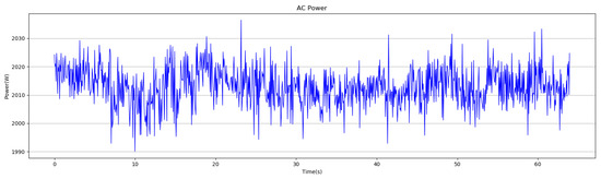
Figure 1. An example of alternating current (AC) power pattern.

In the power pattern in Figure 1, it can be seen that the signals of various sine waves of different sizes have the form of synthesized harmonics. Since the periods of different sine waves are not constant, the power signal has various phase and frequency characteristics. These characteristics contain necessary information for appliance classification because they are inherent characteristics of the appliance when there exist no external factors. In addition, if the power data of a specific appliance is collected for a long period of time (from minutes to years, depending on the data characteristics), it is possible not only to acquire the signal specific characteristics of the appliance, but also to get its power consumption pattern information. So, appliances can be classified more accurately by using them together. Figure 2 shows the daily power consumption pattern of household appliances used in general households. The power input to a household is single-phase AC, but since the power consumption is measured once in a certain period, it becomes a different pattern at a lower sampling rate, where the physical characteristics of the appliances from the AC components may vanish.

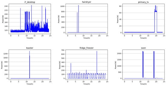
Figure 2. Daily power consumption patterns of home appliances in general households.

In Figure 2, the power consumption pattern can be divided into four types. First, momentary short-time use appliances, such as hair dryers and toasters, have the patterns of pulsing power consumption at the moment of use. Second, appliances that are momentary but constantly used for a period of time, such as televisions and ovens, have a rectangular pattern of power consumption. Thirdly, although they are used continuously, for appliances like a refrigerator, the power consumption pattern varies depending on the driving stage. However, there is a constant power consumption pattern within a certain period. Finally, there is a random power consumption pattern depending on the workload of the program being used, such as the desktop. Since the consumption patterns of the respective appliances may be similar or different from each other according to the appliance usage environment, it may be applied as an approximate classification standard according to the degree of similarity in the appliance classification process. In the classification process, it is possible to roughly classify through the usage pattern of the appliance, and more detailed appliance classification is possible within the roughly classified criteria through the appliance’s inherent power pattern.

2.2. Machine Learning Algorithms for Appliance Classification

In general, the above-mentioned power patterns are used as information to classify appliances. The conventional classification techniques used for NILM are mainly based on the supervised learning. Typical algorithms are: SVM, k-NN algorithm and HMM [9,10,11,14,15,16,17,18,26]. These machine learning techniques have limitations to be applied to the NILM. For example, in the case of SVM, its major problem is that linear SVM is generally limited to two classes. Although it can be extended to more than two classes by using a nonlinear SVM, it has limitations in that nonlinear SVM is difficult to train for larger dataset because it has a training complexity between $\mathcal{O}\left(D^2\right)$ and $\mathcal{O}\left(D^3\right)$ where D is the number of training data. Furthermore, hyper-parameters should be carefully chosen and it is difficult to find the right kernel function [27]. In the case of k-NN algorithm, the performance decreases sharply and the operation takes a long time when the number of classes is large [28,29], which is a significant drawback because the NILM needs to classify unknown number of appliances in typical situations. Finally, in the case of HMM, it has a limitation in that it requires a relatively large number of parameters even for a simple model structure, and it is difficult to learn with a large amount of data [30].

2.3. Deep Learning-Based Approaches

Various studies have been conducted to overcome the limitations of existing classification algorithms for NILM and mainly have been developed based on the use of deep neural networks (DNNs), so-called deep learning, which can analyze the power data more accurately in general [19,20,21,22,23,24]. It has best-in-class performance on problems that significantly outperforms other solutions in multiple different domains including speech recognition, speech synthesis, natural language processing, computer vision, computer games, and so forth, with a significant margin. Also, it has the advantage of not requiring feature engineering and having fixed complexity regardless of amount of the data used for training. However, the main disadvantage of deep learning-based algorithms is that it requires a huge amount of data. Otherwise, it may result in a worse performance than traditional machine learning algorithms. So, a sufficiently large dataset and proper network structure are required for the deep learning-based approaches to be effective.

2.3.1. Recurrent Neural Network

When the power data, temporal data whose values change with time, is input to the most commonly used DNN models such as Convolution Neural Network (CNN) which is specialized in spatial data classification such as images [31], there exist some drawbacks. That is because the most important temporal information from the time series data can not be effectively utilized with a DNN model where data pattern is represented as a whole rather than by time. Therefore, Recurrent Neural Network (RNN) models that efficiently use temporal information for the sequence analysis of input data is applied for classification [32,33,34], because they utilize the past information as well as the current input information for the output of the current state. Figure 3 shows the architecture of a typical RNN model.

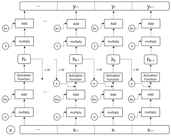
Figure 3. The architecture of a typical RNN model.

In RNN, parameters are learned using Back-Propagation Through Time (BPTT) [35], an extension of the back-propagation algorithm. Essentially BPTT is the same as the basic back-propagation except it carries back-propagation back in time because the RNN structure is linked over time. When the error represented as the cross entropy between the output value and the labeled value, the error for the entire sequence is the total sum of each time step error, and the parameter is updated by calculating the gradient of the error for each parameter in the direction that they are minimized. Here, cross entropy with softmax is used for single-label multi-class classification, and cross entropy with sigmoid is used for multi-label multi-class classification.

2.3.2. Long-Short Term Memory

Typical RNN models have limitations in processing long sequences, that is, if we go through in the order of several steps, the network will no longer retain the previous information. This problem is called long-term dependency problem due to vanishing gradient [36]. As the RNN model becomes deeper, this problem causes fatal errors for the model to learn. So the Long Short-Term Memory (LSTM) was proposed to solve this problem in 1997 by Sepp Hochreiter and Juergen Schmidhuber [37]. LSTM helps the error gradient to flow well back in time by utilizing gates and memory cell. By doing so, the error value is better maintained in the back-propagation step and it remembers its states much longer [38]. The structure of the LSTM consists of one memory cell and three gates: an input gate, a forget gate and an output gate. The input gate controls the range for the new value input to the LSTM and transfers it to the memory cell, and the forget gate controls the memory cell to keep or remove the information. Finally, the output gate controls the range of the output of the current state so that only the desired value can be reflected to the memory cell in the next step, thereby acting role as a long or short memory. The overall operating structure of the LSTM can be expressed by the following equations:

$${\mathit{i}}_{\mathit{t}}={\sigma }_{\mathit{g}}({\mathit{W}}_{\mathit{i}}{\mathit{x}}_{\mathit{t}}+{\mathit{U}}_{\mathit{i}}{\mathit{h}}_{\mathit{t}-1}+{\mathit{b}}_{\mathit{i}})$$

(1)

$${\mathit{f}}_{\mathit{t}}={\sigma }_{\mathit{g}}({\mathit{W}}_{\mathit{f}}{\mathit{x}}_{\mathit{t}}+{\mathit{U}}_{\mathit{f}}{\mathit{h}}_{\mathit{t}-1}+{\mathit{b}}_{\mathit{f}})$$

(2)

$${\mathit{o}}_{\mathit{t}}={\sigma }_{\mathit{g}}({\mathit{W}}_{\mathit{o}}{\mathit{x}}_{\mathit{t}}+{\mathit{U}}_{\mathit{o}}{\mathit{h}}_{\mathit{t}-1}+{\mathit{b}}_{\mathit{o}})$$

(3)

$${\mathit{c}}_{\mathit{t}}={\mathit{f}}_{\mathit{t}}\ast {\mathit{c}}_{\mathit{t}-1}+{\mathit{i}}_{\mathit{t}}\ast {\sigma }_{\mathit{c}}({\mathit{W}}_{\mathit{c}}{\mathit{x}}_{\mathit{t}}+{\mathit{U}}_{\mathit{c}}{\mathit{h}}_{\mathit{t}-1}+{\mathit{b}}_{\mathit{c}})$$

(4)

$${\mathit{h}}_{\mathit{t}}={\mathit{o}}_{\mathit{t}}\ast {\sigma }_{\mathit{h}}\left({\mathit{c}}_{\mathit{t}}\right)$$

(5)

In the above equations, $i_t$, $f_t$, $o_t$, $c_t$ and $h_t$ represent the output of each step at time t and $\sigma$ represents the activation function that operates at each step. W, U and b are weight matrices and bias vector parameters which are updated by training. Figure 4 shows the architecture of LSTM.

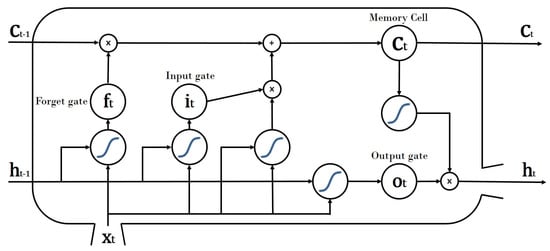
Figure 4. The architecture of LSTM.

Since the power consumption data to be analyzed by NILM process includes signals that have various patterns over various periods, it is necessary to analyze long-term data information in order to analyze them. Therefore, the RNN model is a suitable deep learning model for the classifier of NILM. Based on this, Kim et al. [23,24] proposed a method using RNN to improve the classification performance of NILM. In Reference [23], they used a simple GRU [39] in the appliance classification that showed higher performance than existing classification algorithms such as SVM and HMM. Figure 5 shows the network structure of the GRU. Table 1 shows the performance comparison with the existing classification algorithm as presented in Reference [23].

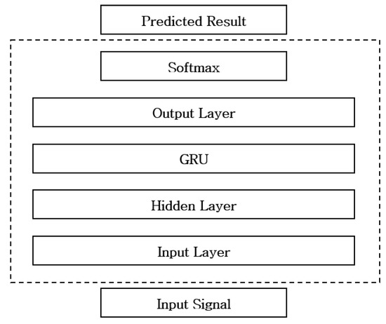
Figure 5. Network structure of GRU.

Table 1. Performance comparison between GRU and other existing algorithms [23].

Classifier Algorithm	Accuracy (%)	F-measure (%)
Bayes	80–92	-
SVM [26]	75–92	-
HMM [14,15]	75–87	-
FHMM [17]	-	80–90
FHMM variants [15]	-	69–98
FHMM using MAP algorithm [14]	71	-
RNN [23]	88–98	77–98
GRU [23]	89–98	81–98

In Reference [24], additional pre-processing to the data is applied before learning the data in the LSTM. In pre-processing, the stronger characteristics of the original signal are enhanced by using the reflectance obtained through the transformed signal of the raw data. These enhanced features are used as a learning guide for data learning. It also shows higher performance than other existing classification algorithms. Figure 6 shows the network structure of the Feature Enhancement Single Layer LSTM (FESL-LSTM) [24].

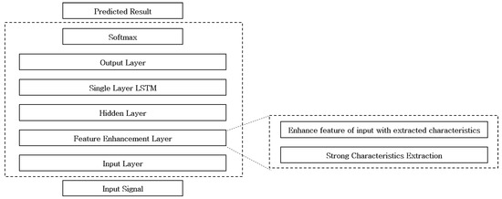
Figure 6. Network structure of the FESL-LSTM.

References [23,24] presented a higher performance than the existing classification algorithms through RNN. However, they did not consider the constraint of the raw data form. In the following section, we present the constraint of the raw data form of the power data and suggest methods to supplement it to better utilize the temporal information for data learning through RNN.

3. Proposed Approach

When using power data as raw data for representing only the time series information, several issues may arise. The power data is sampled in the process of digitizing analog data. By the sampling process, the data become a one-dimensional array having one value at each sampling time. With one-dimensional data typically is very complex, irregular, or difficult to find any patterns (confer Figure 1). It is not a desirable form of data to be used for RNN where we have to find out the patterns of data. To solve this issue, we propose to pre-process the data to use alternative forms of the data as input to RNN. In particular, we used the feature extraction used for transforming time series data in audio signal processing to two-dimensional form. When the data is transformed from one-dimension to two-dimension as a sequence of feature vectors instead of samples, this modified form of data can better represent the data patterns. So more efficient and high-performance learning can be achieved. In addition, by applying such transformations, it is possible to make the learning faster by reducing the data size with an advantage that important information hidden in the data can be better represented for learning. More details about the feature extraction step for our proposed method is described in Section 3.1.

We selected the ML-LSTM model to effectively learn the characteristics of time-series data. Since RNN analyzes data using not only current information but also past information, there is an advantage that it can learn pattern changes according to time changes, but it requires much more information. Therefore, when long-term data is received as input, there is not enough memory to store the data to use the information of the data long ago. LSTM is used as a solution to solve this problem. In addition, by using the LSTM, it is possible to selectively not use unnecessary information from the past information, thereby enabling more efficient learning. However, if the data is very large or contains a lot of important information throughout the data, using only one layer LSTM will not be able to store all the information of the data or will miss important information. For this reason, we used ML-LSTM, which was developed by stacking LSTM in multiple layers.

Overall, we propose the appliance classification network with MFC-ML-LSTM. Figure 7 shows the proposed network structure and Figure 8 shows a block diagram of the proposed appliance classification network.

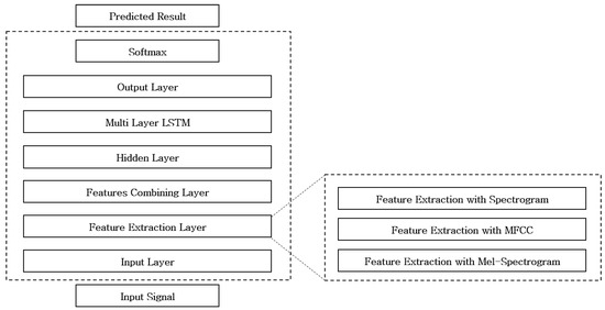
Figure 7. Network structure of MFC-ML-LSTM.

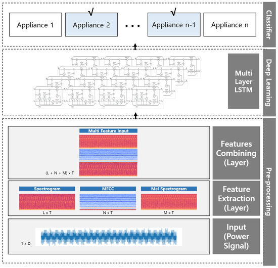
Figure 8. A block diagram of the proposed appliance classification network.

3.1. Feature Extraction

In machine learning, feature extraction starts from an initial set of measured data and builds derived values (features) intended to be informative and non-redundant, facilitating the subsequent learning and generalization steps and in some cases leading to better human interpretations. Feature extraction involves reducing the amount of resources required to describe a large set of data. When performing analysis of complex data one of the major problems stems from the number of variables involved. Analysis with a large number of variables generally requires a large amount of memory and computational power, also it may cause a classification algorithm to overfit to training samples and generalize poorly to new samples. Feature extraction is a general term for methods of constructing combinations of the variables to get around these problems while still describing the data with sufficient accuracy [40,41,42,43]. Optimized feature extraction is the key to effective model construction. There are various approaches to feature extraction. We applied the techniques used in data characterization in audio signal processing to feature extraction of power data. The power data is long sequence data that shows patterns with frequency and time. Therefore, we consider that the feature extraction using the audio signal processing which applies the analysis technique to the characteristics according to the change of the frequency and time of the data will perform better than other feature extraction algorithms. Khunarsal et al. and Raicharoen [44] suggested that, for the classification of sound, all the features extracted through various feature extraction techniques rather than one feature extractor were able to achieve better performance in the overall classification task. As such, we extracted the patterns of power data using three feature extraction techniques which are spectrogram, Mel-Frequency Cepstral Coefficient (MFCC) and Mel-spectrogram after trying various features and then applied them to improve the performance of the classification task.

3.1.1. Spectrogram

A spectrogram is a two-dimensional representation of the magnitude of a signal at various frequencies over time. A spectrogram shows the signal power at each frequency at a particular time as well as how it varies over time. This makes spectrogram an extremely useful tool for the frequency analysis of time-series data. Our work used spectrogram feature analysis based on the Short-Time Fourier transform (STFT) for feature extraction. The STFT is a Fourier transform computed by taking a short segment of a signal typically after applying a window [45]. In practice, the STFT can be obtained by dividing the long-time signal into shorter segments of equal length and calculating the Fourier transform separately in each shorter segment. This represents the Fourier spectrum of each short segment. It then displays the spectra that usually change as a function of time. We can obtain discrete version of STFT in the following equation:

$$\mathit{w}\left[\mathit{n}\right]=0.54-0.46\cos \frac{\pi \mathit{n}}{\mathit{N}},0\le \mathit{n}\le \mathit{N}-1$$

(6)

$$STF{T}_x(m,\omega )=X(m,\omega )=\sum _{n=-\infty }^{\infty }x\left[n\right]w[n-m]e^{-j\omega n}$$

(7)

where $w\left[n\right]$ is the window function with length N that is often taken to be Gaussian window, Hann window or Hamming window: window function is Hamming window in Equation (6) and $x\left[n\right]$ is a discrete-time data at time indexed by an integer n. Finally, the spectrogram can be obtained by logarithmic or linear representation of the spectrum generated by the previous STFT as follows:

$${\mathit{Spectrogram}}_{\mathit{Linear}}(\mathit{m},\mathit{t})=|{\mathit{STFT}}_{\mathit{x}}{(\mathit{m},\omega )|}^2,\forall t$$

(8)

$${\mathit{Spectrogram}}_{\mathit{Log}}(\mathit{m},\mathit{t})=\mathit{Log}\left({\mathit{Spectrogram}}_{\mathit{Linear}}(\mathit{m},\mathit{t})\right),\forall t$$

(9)

Figure 9 shows the block diagram of the spectrogram based on the STFT for feature extraction and Figure 10 shows the waveform and spectrogram of input time series data which is part of the self-configured dataset used in the experiment section.

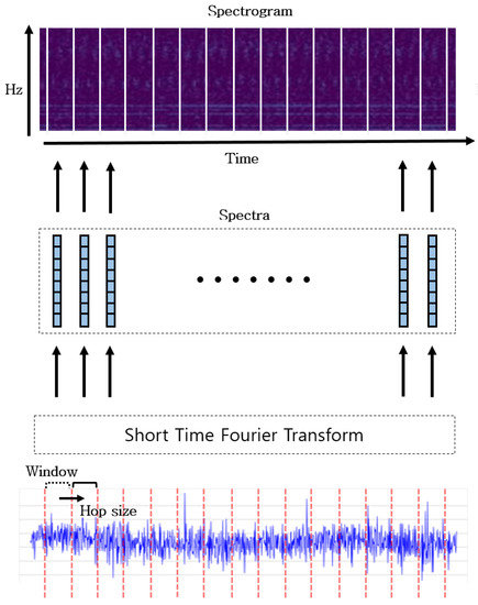
Figure 9. The block diagram of the spectrogram based on STFT.

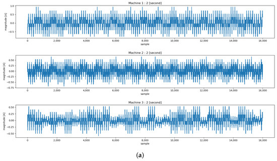
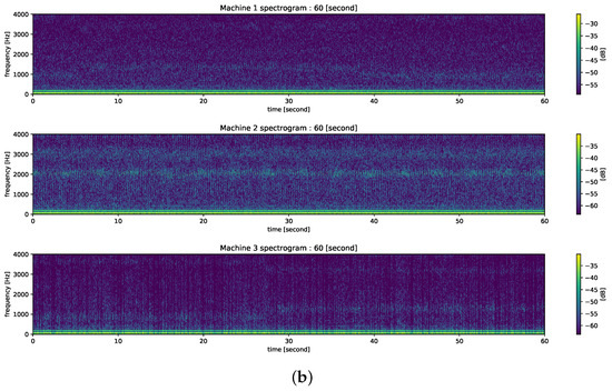
Figure 10. The waveform and spectrogram of input time series data which is part of the self-configured dataset used in the experiment section. (a) The waveform of Machine 1–3’s current for 2 s (16,000 samples). (b) The spectrogram of Machine 1–3’s current for 60 s.

3.1.2. Mel-Spectrogram and MFCC

Human perception of the frequency content of sound for an audio signal does not follow the linear scale. Thus, for each tone with the actual pitch f measured in Hz, the subjective pitch is measured on a scale called a ‘Mel’ scale. The Mel-frequency scale is a linear frequency interval of 1000 Hz or less and a log interval of 1000 Hz or higher [46]. On Mel-frequency scale, spectrum is transformed into Mel-spectrum through Mel-filter banks of triangular overlapping windows. The Mel-filter bank is a critical band with various bandwidth on normal frequency scale and emphasizes information in the low frequency range by placing a large number of filters in low frequency bands than high frequency bands. Mel-spectrogram generated in this manner focuses more on the low frequency patterns than the higher frequency patterns of the power signal with the reduced dimension. Although the Mel-spectrogram is motivated by human perception of audio frequency, we believe that this conversion is useful for power data analysis because the lower frequency patterns may also carry crucial information than higher frequency patterns. At the same time, higher frequency patterns may also contribute to the information, less importantly than the lower frequency patterns, making the Mel-spectrogram a useful choice for the classification task.

Mel Frequency Cepstral Coefficients (MFCC) can be obtained by converting the logarithm of the Mel-spectrum back to time with a discrete cosine transform (DCT) [46]. By converting the logarithm of the Mel-spectrum, low-frequency information is extended, and the MFCC has only a real part because of DCT. It can be expressed by the following equation:

$${\mathit{c}}_{\mathit{n}}=\sum _{\mathit{k}=1}^{\mathit{K}}\left(\log {\mathit{s}}_{\mathit{k}}\right)\cos \left[\mathit{n}(\mathit{k}-0.5)\frac{\pi }{\mathit{K}}\right],\mathrm{for}\mathit{n}=1,\dots ,\mathit{N},$$

(10)

where $s_k$ is the output power of the kth filter of the filter bank and $c_n$ is the obtained MFCC with N number of parameters through DCT. Figure 11 shows the Block diagram of MFCC.

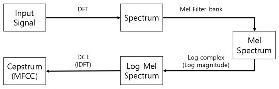
Figure 11. The Block diagram of MFCC.

One of the advantages of the MFCC is that it deconvolves convoluted signal into individual components [45] and although it was originally developed for speech analysis [46], we believe that it works well for power signal analysis because power signals may also contain convolutive components.

3.2. Multiple Feature Combination

We use three data feature extraction techniques for better appliance classification performance as described in Section 3.1. However, unlike the existing method [44], each data obtained through three feature extraction is not inputted as one data independently, but the data generated after three feature extraction are combined into one data as input. When each data is used independently, it is difficult to optimize the trained parameters of the deep learning to values that satisfy all of the different data types. Therefore, it is possible to learn data more efficiently by using it as a single data. The combination of data is a simple concatenation. First, when each feature extraction technique is applied to the raw data, the parameters of each feature extraction technique are set so that the temporal dimension can be generated equally to constitute as one set. The next step is to stack the data up in temporal order. This set of data is one input. In this paper, data were stacked in the order of spectrogram, MFCC and Mel-spectrogram. The data concatenation can be expressed as follows:

$$\begin{array}{c}\hfill x^{\left(1\right)}=\mathrm{Spectrogram}\in {\mathcal{R}}^{L\times T}\end{array}$$

(11)

$$x^{\left(2\right)}=\mathrm{MFCC}\in {\mathcal{R}}^{N\times T}$$

(12)

$$x^{\left(3\right)}=\mathrm{Mel}-\mathrm{Spectrogram}\in {\mathcal{R}}^{K\times T}$$

(13)

$$x=[x_1,x_2,\dots ,x_T]=\left[\begin{array}{c}{x}^{\left(1\right)}\\ x^{\left(2\right)}\\ x^{\left(3\right)}\end{array}\right]\in {\mathcal{R}}^{(L+N+K)\times T},$$

(14)

where L, N, and K are the feature vector sizes of spectrogram, MFCC, and Mel-spectrogram respectively. At each time t, the column vector $x_t$ of size $(L+N+K)\times 1$ is used as the input to the RNN structure (confer Figure 3). Figure 12 shows the combined features for some appliances along with the raw data.

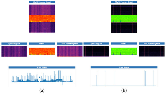
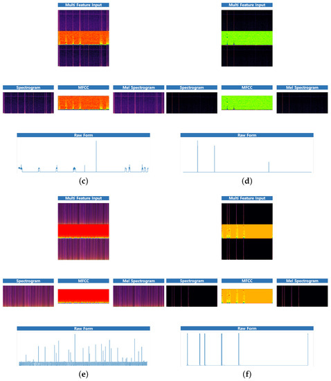
Figure 12. The feature combination of some appliances with original signal. (a) i7_desktop (b) hairdryer (c) primary_tv (d) toaster (e) fridge_freezer (f) oven.

4. Experiments

We constructed experiments to verify the validity and the performance of the proposed model, MFC-ML-LSTM. The experimental configuration consisted of four performance comparison works. First, we compare the performance of raw data and spectrogram as input by using a self-configured dataset. Second, we compare the performance of the CNN model with our ML-LSTM model using the spectrogram of the self-configured dataset. Third, we compared the performances of the MFC input consisting of spectrogram, MFCC and Mel-spectrogram with only the spectrogram input using the UK-DALE-2017 dataset. These three comparison works are done for the task of single-label multi-class classification, where a single appliance is identified among multiple appliances from the power data of a single unknown appliance. Finally, we compare the performance of our proposed model with the existing methods presented in other works [23,24] for the multi-label multi-class classification, where one or more unknown number of appliances are identified from aggregated power data of unspecified number of appliances.

4.1. Dataset Description

We constructed two sets of data to validate our results by applying our work to real data. One is a self-configured dataset for experimentation and the other is the UK-DALE-2017 dataset, a public dataset for NILM.

4.1.1. Self-Configured Dataset

We configured our own dataset for performance evaluation of data with high sampling rate. Data have been collected from three different factory equipment’s motor at a sampling rate of 8 kHz, and the values of three-phase, four-wire current and voltage for each equipment were recorded. When comparing the amount of information for the same time with the data with low sampling rate, the data with high sampling rate has the disadvantage that it needs a lot of memory for higher data capacity in the classification work but has the advantage that it can achieve better performance because it utilizes more information.

4.1.2. UK-DALE-2017 Dataset

The UK-DALE-2017 dataset was proposed by Jack Kelly and William Knottenbelt and it was released in 2014 at first and it has been updated every year [25]. It is an open-access dataset from the UK recording Domestic Appliance-Level Electricity at a sample rate of 16 kHz for the whole-house and at 1/6 Hz for individual appliances. But, the 16 kHz data was not used in this paper because the difference in data recording periods for each appliance is so large, this data unbalance can bring about overfitting problems in training with deep learning and we also have focused more on the user’s appliance usage pattern. Therefore, we use only 1/6 Hz data. There are power data for five houses, each house has information about the different kinds and number of appliances, and the recording duration of each house and appliance is different. In our experiments, we did not use data which don’t label properly or have a very little amount of data compared to other appliances. Table 2 shows the detailed description of UK-DALE-2017 dataset and Table 3 shows the list of appliances selected for learning with UK-DALE-2017 dataset.

Table 2. The detailed description of UK-DALE-2017 dataset.

House	Building of Type	Duration of Recording (Days)	Number of Appliance	Number of Using Appliance	Sample Rate
1	End of terrace	786	53	31	16 kHz, 1 Hz, 1/6 Hz
2	End of terrace	234	20	12	16 kHz, 1 Hz, 1/6 Hz
3	-	39	5	2	1/6 Hz
4	Mid-terrace	205	6	2	16 kHz, 1 Hz, 1/6 Hz
5	flat	137	26	15	1/6 Hz

Table 3. The list of appliances selected for learning in UK-DALE-2017 dataset.

House	Appliance
1	dishwasher, amp_livingroom, kitchen_dt_lamp, livingroom_lamp_tv, washing_machine, battery_charger, office_lamp3, livingroom_s_lamp, kitchen_lamp2, livingroom_s_lamp2, gigE_&_USBhub, solar_thermal_pump, fridge, samsung_charger, htpc, hifi_office, gas_oven, subwoofer_livingroom, tv, office_pc, bedroom_chargers, lighting_circuit, laptop, kitchen_lights, office_lamp1, lcd_office, adsl_router, kitchen_phone&stereo, childs_ds_lamp, data_logger_pc, office_lamp2
2	server, dish_washer, laptop2, router, fridge, modem, washing_machine, monitor, running_machine, microwave, server_hdd, speakers
3	electric_heater, laptop
4	gas_boiler, freezer
5	core2_server, microwave, washer_dryer, i7_desktop, network_attached_storage, dishwasher, sky_hd_box, 24_inch_lcd_bedroom, fridge_freezer, oven, 24_inch_lcd, treadmill, atom_pc, home_theatre_amp, primary_tv

4.2. Data Processing and Setup

We have worked to fit the dataset into our framework for multi-class classification as follows (the entire process is done independently for each house in the UK-DALE-2017 dataset and each factory equipment in the self-configured dataset):

• Define the data size by cutting a time series data for each appliance class every duration L with stride M (overlapping $L-M$) and then cut the data as defined.
• If non-zero data is less than 1% of the duration L, the data is additionally labeled as ‘None’.
• Labeling each class about appliance by one-hot encoding.
• The datasets of each class about appliance are collected and shuffled randomly.
• The datasets are divided into train, validation and test sets with the ratio of 60:20:20.

In order to increase the amount of data, we truncated the stride to less than time L so that the data cut in step 1 of the process can be overlapped. By doing this, not only the amount of data increases, but also the important front and back information relation of the serial data can be maintained naturally. Table 4 shows time L, M for each dataset setting and Table 5 and Table 6 show the overall dataset configuration.

Table 4. The time L, M for each dataset setting.

Dataset	L (One Data Duration)	M (Stride)	L-M (Overlapping)
UK-DALE-2017	24 h	12 h	12 h
Self-configured	3 s	2 s	1 s

Table 5. The number of extracted data for each house of UK-DALE-2017 dataset.

House	# of Train (+Validation)	# of Test
House 1	75,771	18,923
House 2	3659	909
House 3	112	28
House 4	724	180
House 5	3413	849

Table 6. The number of extracted data for each feature of self-configured dataset.

# of Train	# of Validation	# of Test
10,912	3632	3648

Since UK-DALE-2017 dataset recorded at 1/6 Hz contains only individual directly measured data for each appliance, it does not include any aggregated data. So for multi-label classification, the data from individual appliances should be combined together. In order to maintain the balance among different classes, the data mixing process for combining data of different appliances considers the frequency of usage for each appliance. The specific data mixing procedure is as follows.

• Define the data size by cutting a time series data for each appliance class every duration 24 h with stride 12 h (overlapping 12 h) and then cut the data as defined (as Table 4).
• If non-zero data is less than about 30 s of duration 24 h, the data is removed.
• Obtains the number of data of each appliance generated through steps 1, 2.
• The dataset is divided into train (+ validation) set and test set at a ratio of 80:20.
• (For each set) After finding the number of appliances with the highest number of data, fill the data with only as few as zero for the appliance with a lower number of data and shuffle randomly.
• (For each set) To create various mixing patterns, randomly shuffle the data generated in step 5 and attach it to the back of the existing data.
• (For each set) Mix all the appliance data with simple addition and label with multi-hot encoding.
• (For each set) Add independent data of each appliance that is not mixed to set.

Since the measurement duration of the power used by each appliance and the measurement start time are different, it is necessary to adjust the total duration of the data to be mixed as in the above-mentioned step 4 in data mixing. And, since the measurement duration of each of the appliances is different but there is not much difference except for a few, it makes possible that the user’s usage frequency information of data can be mixed similarly to the actual data by filling with zero to the data of the insufficient duration and shuffling randomly. In step 5, data before mixing is added to the train set to improve classification performance, and also added to the test set to check the performance of the single appliance event. Figure 13 shows the diagram of the data mixing process and Figure 14 shows some mixed data plots.

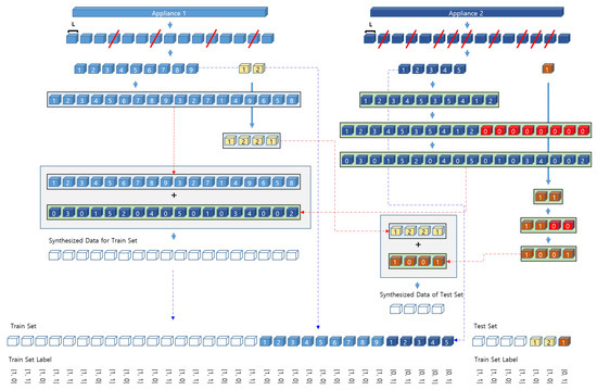
Figure 13. The diagram of the data mixing process.

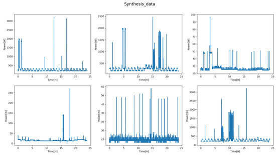
Figure 14. Some mixed data plots.

4.3. Experiment Environment

We used the Tensorflow framework for deep learning and the specification of our workstation for training the proposed model is as follows:

• CPU: Intel (R) Xeon (R) CPU E5 – 2603 v3 @ 1.60Hz (12 cores)
• GPU: GeForce GTX TITAN X (x 4)
• RAM: 64 GB
• OS: Ubuntu 14.04.5 LTS

4.4. The Hyperparameters for Learning

The hyper parameter is a key factor that affects the algorithm’s performance. Depending on how the hyper parameters are configured, data learning time, memory capacity, and learning outcomes can change significantly. We were able to achieve better performance by adjusting hyper parameters such as learning rate, hidden layer size, ML-LSTM layer sizes, batch sizes and epochs. Our Hyper parameter settings are shown in Table 7.

Table 7. Hyper parameter settings for learning.

Hyper Parameter	Value	Explanation
Learning rate	0.0001	The ratio to reach for the optimum set of parameters. It affects the optimization speed of deep learning model through the optimizer.
Hidden layer size	256	The number of the hidden layer’s nodes. It affects the learning depth of deep learning.
Optimizer	Adam	A parameter optimization model. Adam Optimizer is one of the most popular optimizers in deep learning as it adjusts the update level of learning rate by calculating the optimization speed of parameters while reducing learning rate during training.
ML-LSTM layer size	6	The number of stacked LSTM layers. As the more layers, the LSTM can store more information.
Batch size	20	The size of the batch which is a way of learning various information at the same time by grouping multiple inputs rather than one input.
Epochs	600	A unit for the process of learning with the whole data once in the training dataset.

4.5. Evaluation Methods of Performance

For our model performance evaluation, we measured the micro-average of the Precision, Recall, F1-Score and Accuracy by using the confusion matrix which is proposed by Kohavi and Provost [47], as shown in Table 8.

Table 8. The confusion matrix.

	Predicted	Yes	No
Label
Yes		TP	FN
No		FP	TN

Where, TP is “true positive” for correctly predicted event, FP is “false positive” for incorrectly predicted event, TN is “true negative” for correctly predicted non-event, and FN is “false negative” for incorrectly predicted non-event. The Precision, Recall, F1-Score and Accuracy are defined as follows:

$$\mathit{Precision}=\frac{\mathit{TP}}{\mathit{TP}+\mathit{FP}}$$

(15a)

$$\mathit{Recall}=\frac{\mathit{TP}}{\mathit{TP}+\mathit{FN}}$$

(15b)

$${\mathit{F}}_1-\mathit{Score}=2\ast \frac{\mathit{Precision}\ast \mathit{Recall}}{\mathit{Precision}+\mathit{Recall}}$$

(15c)

$$\mathit{Accuracy}=\frac{\mathit{TP}+\mathit{TN}}{\mathit{TP}+\mathit{FP}+\mathit{FN}+\mathit{TN}}$$

(15d)

5. Results and Discussion

5.1. Performance Comparison between Raw Data and Spectrogram

In this experiment, we use the self-configured dataset to verify the importance of the input data type. We used ML-LSTM model for single-label multi-class classification for both raw data and spectrogram. Since the raw data is a 1-D array, we divide the values according to each time into specific period units and use it as information in each step of RNN to add more information at each step. Figure 15 shows the results of using raw data and spectrogram as input.

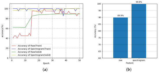
Figure 15. The training and test results for raw data and spectrogram of self-configured dataset as the input to an ML-LSTM model. (a) The training result in terms of the accuracy with respect to the number of epochs. (b) The test result in accuracy.

Figure 15b shows that with the raw data as input, the training accuracy begins at about 40% whereas with the spectrogram as input, the training accuracy begins at about 100%. This confirms that the spectrogram carries more prominent patterns of the data for classification. Also, the results of each test show that when the spectrogram was the input, the performance of the classification accuracy is higher at 99.8%. Although there are only three classes for classification with the self-configured dataset, we confirm that the performance is better with the spectrogram than the raw data as input.

5.2. Performance Comparison between CNN and RNN

In this experiment, we compare the RNN model with the CNN model by using the spectrogram as input using the self-configured dataset. The spectrogram is used because it performs better than the raw data and is a two-dimensional format suitable for training with the CNN, and CNN uses a structure that extends the filter size of the convolution layer to $5\times 5$ of the LeNet5. Figure 16 shows training and test results for the CNN and the RNN where ML-LSTM was used as the RNN model.

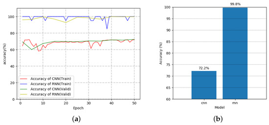
Figure 16. The training and test results for CNN and RNN using spectrogram of self-configured dataset. (a) The training result in terms of the accuracy with respect to the number of epochs. (b) The test result in accuracy.

Figure 16a shows that, at the beginning of the training, RNN achieves close to 100% training accuracy contrary to the CNN model which achieves about 73%, even though it is a popularly used model for image classification tasks. Also, Figure 16b shows that the performance of the CNN is significantly lower than that of the RNN. This is because it can not fully utilize the temporal information of the power data for learning. It is possible that the performance is poor because we used CNN’s basic network structure (LeNet5). Nevertheless, we believe that using RNN will perform still better than using other advanced CNN structure. Because the power data has values according to certain patterns according to time, the RNN model is shown to be more suitable than the CNN model.

5.3. Performance Comparison between Single Input and Multiple Feature Combination Input

Previous experiments have shown that the use of RNN and spectrogram are suitable choices for power data. Based on this, in this experiment, we compared the performance of the reconstructed MFC input network with that of the single input network by adding other feature extraction techniques to confirm that the performance improves when the input data consist of the combination of multiple features (spectrogram, MFCC, Mel-spectrogram) instead of single feature (only spectrogram). The Figure 17 shows the results for the performance based on the input settings about UK-DALE-2017 dataset. For multiple features, each feature is combined into a feature set by simple concatenation.

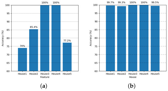
Figure 17. The results of the performance based on the input settings of the UK-DALE-2017 dataset. (a) Result of performance in terms of the accuracy when the input is only spectrogram. (b) Result of performance in terms of the accuracy when the input is the multiple feature combination of Spectrogram, MFCC, Mel-spectrogram.

The MFC performed much better than the spectrogram as the input. Although we did not experiment with different combinations of features that had the highest performance in paper proposed by Khunarsal et al. and Raicharoen [44], we already achieved much higher results as shown in Figure 17b that the accuracy for each house is close to 100%. Regarding this single-label multi-class classification task, the confusion matrix and F1-score of each appliance of House 2 of UK-DALE-2017 dataset are given in Table 9.

Table 9. The confusion matrix and F1-score of each appliance in House 2.

	Predicted	Monitor	Speakers	Server	Router	Server_Hdd	Kettle	Rice_Cooker	Running_Machine	Laptop2	Washing_Machine	Dish_Washer	Fridge	Microwave	Toaster	Playstation	Modem	None	F1-Score
Label
monitor		62	0	0	0	1	0	0	0	4	0	0	0	0	0	0	0	0	0.939
speakers		0	70	2	2	0	0	0	3	0	0	0	0	0	0	0	0	0	0.933
server		0	0	77	0	0	0	0	0	0	0	0	0	0	0	0	0	0	0.962
router		0	1	0	73	0	0	0	0	0	1	0	0	0	0	0	2	0	0.907
server_hdd		1	0	0	0	40	0	0	0	0	0	4	0	0	0	0	0	0	0.909
kettle		0	0	0	0	0	56	1	0	0	0	0	0	0	0	0	0	0	0.974
rice_cooker		0	0	0	0	0	2	53	2	0	0	0	0	0	0	0	0	0	0.955
running_machine		0	2	4	0	0	0	0	51	0	0	0	0	0	0	0	0	0	0.895
laptop2		2	0	0	0	0	0	0	0	46	1	0	0	0	0	0	0	1	0.920
washing_machine		0	0	0	8	0	0	0	0	0	38	0	0	0	0	0	0	0	0.884
dish_washer		0	0	0	0	2	0	0	0	0	0	44	0	0	0	0	0	0	0.936
fridge		0	0	0	0	0	0	0	0	0	0	0	46	0	0	0	0	0	1.000
microwave		0	0	0	0	0	0	0	0	0	0	0	0	2	0	0	0	7	0.222
toaster		0	0	0	0	0	0	0	0	0	0	0	0	0	46	0	0	0	1.000
playstation		0	0	0	0	0	0	0	1	0	0	0	0	0	0	45	0	0	0.989
modem		0	0	0	1	0	0	0	0	0	0	0	0	0	0	0	45	0	0.968
none		0	0	0	0	0	0	0	0	0	0	0	0	7	0	0	0	53	0.876

5.4. Performance Comparison between Existing RNN Models and the Proposed Model

Finally, in this experiment, the performance of our proposed model, MFC-ML-LSTM, is compared with other models, GRU [23] and FESL-LSTM [24], for multi-label classification. Figure 18 shows the accuracy comparison result and Figure 19 shows the F1-score comparison result. Table 10 shows the multi-label classification result of each appliance in House 1 of the mixed data using UK-DALE-2017 dataset as described in Section 4.2.

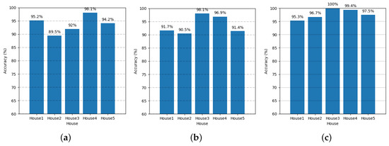
Figure 18. The multi-label classification results of the mixed data using UK-DALE-2017 dataset. The accuracy of (a) GRU, (b) FESL-LSTM, and (c) MFC-ML-LSTM.

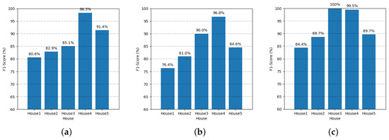
Figure 19. The multi-label classification results of the mixed data using UK-DALE-2017 dataset. The F1-score of (a) GRU, (b) FESL-LSTM, and (c) MFC-ML-LSTM.

Table 10. The multi-label classification result of each appliance in House 1.

Appliance	F1-Score	Accuracy	Appliance	F1-Score	Accuracy
dishwasher	91.96%	97.66%	subwoofer_livingroom	99.74%	99.89%
amp_livingroom	97.93%	99.10%	tv	99.60%	99.83%
kitchen_dt_lamp	44.82%	91.95%	office_pc	50.45%	94.26%
livingroom_lamp_tv	87.78%	95.04%	bedroom_chargers	62.14%	89.96%
battery_charger	40.98%	93.06%	lighting_circuit	97.98%	99.12%
office_lamp3	47.50%	94.43%	laptop	63.73%	94.42%
livingroom_s_lamp	84.32%	93.97%	kitchen_lights	98.17%	99.21%
kitchen_lamp2	47.66%	91.43%	office_lamp1	40.77%	90.15%
livingroom_s_lamp2	73.84%	91.21%	lcd_office	49.30%	93.10%
gigE_&_USBhub	45.73%	92.98%	adsl_router	98.58%	99.38%
solar_thermal_pump	99.16%	99.63%	kitchen_phone&stereo	69.34%	90.37%
fridge	99.96%	99.98%	childs_ds_lamp	77.00%	99.22%
samsung_charger	77.45%	92.33%	data_logger_pc	99.86%	99.94%
htpc	98.92%	99.53%	office_lamp2	52.97%	88.29%
hifi_office	48.82%	93.58%	washing_machine	93.28%	97.54%
gas_oven	99.04%	99.58%

As shown in Figure 18, the accuracy of MFC-ML-LSTM is shown to be higher than the others for all houses. The F1-score is also higher than that of the others, except for House 5, as shown in Figure 19. These results show that our proposed model has better performance for multi-label classification. As F1-score in Table 10 shows, the experimental results for all houses show that appliances having a small power consumption patterns based a pulse shape such as lamp cannot be classified well if those are mixed together with appliances that have high power consumption patterns at all times such as fridge or PC. This, of course, is because a small signal with a simple pulse pattern is masked by being mixed into significantly larger signal. However, even if a signal has such a simple pulse pattern, it can be confirmed that the signal is classified better when the amplitude of the signal is larger than that of the other mixed signals altogether.

6. Conclusions

This paper proposed a new RNN-based network for appliance classification—namely MFC-ML-LSTM—in order to overcome the limitations of existing classification algorithms. By applying various feature extraction techniques commonly used for audio signal processing to the ML-LSTM, it achieves superior classification performance to the existing RNN-based methods. In particular, by using the combination of the spectrogram providing the spectral pattern of the power data, the Mel-Spectrogram focusing more on the lower frequency range than the higher frequency range, and the MFCC deconvolving any convolved components of the power data, the representation of power data specific to the individual appliances become more apparent, resulting in more accurate classification. Furthermore, the amount of information used for learning can be increased by combining multiple features as a single input.

Experimental results verified the assumptions presented in this paper and then compared the performance of the MFC-ML-LSTM with the existing RNN based models, GRU and FESL-LSTM. They show that the proposed method achieves the accuracy and the F1-score improvements of 0.1% to 10% compared with other existing RNN-based models. In particular, the proposed method achieved accuracy more than 95%, which is significantly high for appliance classification.

For multi-label multi-class classification, artificially generated data were used to avoid data unbalance and labeling issues. It is anticipated that the performance may get worse if real aggregate data are used because actual data may contain unknown patterns due to various external factors unlike the mixed data as a simple sum of individual power data. Since the proposed approach tries to combine multiple different representations of the power data, we expect that it may still work well, which can be verified with the help of properly labeled aggregated data collected in real-world scenarios.

There are various power data depending on the environment in which NILM is applied. Therefore, there exist more cases that can significantly benefit from the proper choices of feature extraction techniques. Regarding this, we plan to investigate more powerful representations of the power data by exploring proper frequency ranges and other feature extraction techniques in the feature extraction layer and by changing the number, combinations, and dimension of the features in the feature combining layer of the MFC-ML-LSTM.

References

- Hart, G.W. Nonintrusive appliance load monitoring. Proc. IEEE 1992, 80, 1870–1891. [Google Scholar] [CrossRef]
- Zeifman, M.; Roth, K. Nonintrusive appliance load monitoring: Review and outlook. IEEE Trans. Consum. Electron. 2011, 57, 76–84. [Google Scholar] [CrossRef]
- Singh, J.K. Managing Power Consumption Based on Utilization Statistics. U.S. Patent 6,996,728, 7 February 2006. [Google Scholar]
- Hunter, R.R. Method and Apparatus for Reading and Controlling Electric Power Consumption. U.S. Patent 7,263,450, 28 August 2007. [Google Scholar]
- Forth, B.J.; Cowan, P.C.; Giles, D.W.; Ki, C.S.S.; Sheppard, J.D.; Van Gorp, J.C.; Yeo, J.W.; Teachman, M.E.; Gilbert, B.J.; Hart, R.G.; et al. Intra-Device Communications Architecture for Managing Electrical Power Distribution and Consumption. U.S. Patent 6,961,641, 1 November 2005. [Google Scholar]
- He, D.; Du, L.; Yang, Y.; Harley, R.; Habetler, T. Front-end electronic circuit topology analysis for model-driven classification and monitoring of appliance loads in smart buildings. IEEE Trans. Smart Grid 2012, 3, 2286–2293. [Google Scholar] [CrossRef]
- Li, J.; West, S.; Platt, G. Power decomposition based on SVM regression. In Proceedings of the 2012 International Conference on Modelling, Identification and Control, Wuhan, China, 24–26 June 2012; pp. 1195–1199. [Google Scholar]
- Jiang, L.; Luo, S.; Li, J. An approach of household power appliance monitoring based on machine learning. In Proceedings of the 2012 Fifth International Conference on Intelligent Computation Technology and Automation, Zhangjiajie, China, 12–14 January 2012; pp. 577–580. [Google Scholar]
- Figueiredo, M.; De Almeida, A.; Ribeiro, B. Home electrical signal disaggregation for non-intrusive load monitoring (NILM) systems. Neurocomputing 2012, 96, 66–73. [Google Scholar] [CrossRef]
- Figueiredo, M.B.; De Almeida, A.; Ribeiro, B. An experimental study on electrical signature identification of non-intrusive load monitoring (nilm) systems. In Proceedings of the International Conference on Adaptive and Natural Computing Algorithms, Ljubljana, Slovenia, 14–16 April 2011; pp. 31–40. [Google Scholar]
- Makonin, S. Approaches to Non-Intrusive Load Monitoring (NILM) in the Home; Technical Report; Simon Fraser University: Burnaby, BC, Canada, 24 October 2012. [Google Scholar]
- Kang, S.; Yoon, J.W. Classification of home appliance by using Probabilistic KNN with sensor data. In Proceedings of the 2016 Asia-Pacific Signal and Information Processing Association Annual Summit and Conference (APSIPA), Jeju, Korea, 13–16 December 2016; pp. 1–5. [Google Scholar]
- Batra, N.; Singh, A.; Whitehouse, K. Neighbourhood nilm: A big-data approach to household energy disaggregation. arXiv 2015, arXiv:1511.02900. [Google Scholar]
- Kolter, J.Z.; Jaakkola, T. Approximate inference in additive factorial hmms with application to energy disaggregation. Artif. Intell. Stat. 2012, 22, 1472–1482. [Google Scholar]
- Kim, H.; Marwah, M.; Arlitt, M.; Lyon, G.; Han, J. Unsupervised disaggregation of low frequency power measurements. In Proceedings of the 2011 SIAM International Conference on Data Mining (SIAM), Mesa, AZ, USA, 28–30 April 2011; pp. 747–758. [Google Scholar]
- Makonin, S.; Bajic, I.V.; Popowich, F. Efficient sparse matrix processing for nonintrusive load monitoring (NILM). In Proceedings of the 2nd International Workshop on Non-Intrusive Load Monitoring, Austin, TX, USA, 3 June 2014. [Google Scholar]
- Zoha, A.; Gluhak, A.; Nati, M.; Imran, M.A. Low-power appliance monitoring using factorial hidden markov models. In Proceedings of the 2013 IEEE Eighth International Conference on Intelligent Sensors, Sensor Networks and Information Processing, Melbourne, Australia, 2–5 April 2013; pp. 527–532. [Google Scholar]
- Mauch, L.; Barsim, K.S.; Yang, B. How well can HMM model load signals. In Proceedings of the 3rd International Workshop on Non-Intrusive Load Monitoring (NILM 2016), Vancouver, BC, Canada, 14–15 May 2016. Number 6. [Google Scholar]
- Kelly, J.; Knottenbelt, W. Neural nilm: Deep neural networks applied to energy disaggregation. In Proceedings of the 2nd ACM International Conference on Embedded Systems for Energy-Efficient Built Environments, Seoul, Korea, 4–5 November 2015; pp. 55–64. [Google Scholar]
- De Baets, L.; Ruyssinck, J.; Develder, C.; Dhaene, T.; Deschrijver, D. Appliance classification using VI trajectories and convolutional neural networks. Energy Build. 2018, 158, 32–36. [Google Scholar] [CrossRef]
- De Baets, L.; Dhaene, T.; Deschrijver, D.; Berges, M.; Develder, C. VI-based appliance classification using aggregated power consumption Data. In Proceedings of the 4th IEEE International Conference on Smart Computing (SMARTCOMP 2018), Taormina, Italy, 18–20 June 2018; pp. 1–8. [Google Scholar]
- De Paiva Penha, D.; Castro, A.R.G. Convolutional neural network applied to the identification of residential equipment in non-intrusive load monitoring systems. In Proceedings of the 3rd International Conference on Artificial Intelligence and Applications, Chennai, India, 30–31 December 2017; pp. 11–21. [Google Scholar]
- Kim, J.; Kim, H. Classification performance using gated recurrent unit recurrent neural network on energy disaggregation. In Proceedings of the 2016 International Conference on Machine Learning and Cybernetics (ICMLC), Jeju Island, Korea, 10–13 July 2016; Volume 1, pp. 105–110. [Google Scholar]
- Kim, J.; Le, T.T.H.; Kim, H. Nonintrusive load monitoring based on advanced deep learning and novel signature. Comput. Intell. Neurosci. 2017, 2017, 4216281. [Google Scholar] [CrossRef] [PubMed]
- Kelly, J.; Knottenbelt, W. The UK-DALE dataset, domestic appliance-level electricity demand and whole-house demand from five UK homes. Sci. Data 2015, 2, 150007. [Google Scholar] [CrossRef] [PubMed]
- Kato, T.; Cho, H.S.; Lee, D.; Toyomura, T.; Yamazaki, T. Appliance recognition from electric current signals for information-energy integrated network in home environments. In Proceedings of the International Conference on Smart Homes and Health Telematics, Tours, France, 1–3 July 2009; pp. 150–157. [Google Scholar]
- Kotsiantis, S.B.; Zaharakis, I.; Pintelas, P. Supervised machine learning: A review of classification techniques. Emerg. Artif. Intell. Appl. Comput. Eng. 2007, 160, 3–24. [Google Scholar]
- Zhang, M.L.; Zhou, Z.H. A k-nearest neighbor based algorithm for multi-label classification. In Proceedings of the 2005 IEEE International Conference on Granular Computing, Beijing, China, 25–27 July 2005; Volume 2, pp. 718–721. [Google Scholar]
- Laaksonen, J.; Oja, E. Classification with learning k-nearest neighbors. In Proceedings of the IEEE International Conference on Neural Networks, Washington, DC, USA, 3–6 June 1996; Volume 3, pp. 1480–1483. [Google Scholar]
- Rabiner, L.R.; Juang, B.H. An introduction to hidden Markov models. IEEE ASSP Mag. 1986, 3, 4–16. [Google Scholar] [CrossRef]
- Wang, J.; Yang, Y.; Mao, J.; Huang, Z.; Huang, C.; Xu, W. Cnn-rnn: A unified framework for multi-label image classification. In Proceedings of the IEEE Conference on Computer Vision and Pattern Recognition, Las Vegas, NV, USA, 26 June–1 July 2016; pp. 2285–2294. [Google Scholar]
- Giles, C.L.; Miller, C.B.; Chen, D.; Sun, G.Z.; Chen, H.H.; Lee, Y.C. Extracting and learning an unknown grammar with recurrent neural networks. In Proceedings of the Advances in Neural Information Processing Systems, Denver, CO, USA, 30 November–3 December 1992; pp. 317–324. [Google Scholar]
- Lawrence, S.; Giles, C.L.; Fong, S. Natural language grammatical inference with recurrent neural networks. IEEE Trans. Knowl. Data Eng. 2000, 12, 126–140. [Google Scholar] [CrossRef]
- Watrous, R.L.; Kuhn, G.M. Induction of finite-state languages using second-order recurrent networks. Neural Comput. 1992, 4, 406–414. [Google Scholar] [CrossRef]
- Werbos, P.J. Backpropagation through time: what it does and how to do it. Proc. IEEE 1990, 78, 1550–1560. [Google Scholar] [CrossRef]
- Bengio, Y.; Simard, P.; Frasconi, P. Learning long-term dependencies with gradient descent is difficult. IEEE Trans. Neural Netw. 1994, 5, 157–166. [Google Scholar] [CrossRef] [PubMed]
- Hochreiter, S.; Schmidhuber, J. Long short-term memory. Neural Comput. 1997, 9, 1735–1780. [Google Scholar] [CrossRef] [PubMed]
- Gers, F.A.; Schraudolph, N.N.; Schmidhuber, J. Learning precise timing with LSTM recurrent networks. J. Mach. Learn. Res. 2002, 3, 115–143. [Google Scholar]
- Cho, K.; Van Merriënboer, B.; Bahdanau, D.; Bengio, Y. On the properties of neural machine translation: Encoder-decoder approaches. arXiv 2014, arXiv:1409.1259. [Google Scholar]
- Guyon, I.; Elisseeff, A. An introduction to feature extraction. In Feature Extraction; Springer: Berlin, Germany, 2006; pp. 1–25. [Google Scholar]
- Kumar, S.; Ghosh, J.; Crawford, M.M. Best-bases feature extraction algorithms for classification of hyperspectral data. IEEE Trans. Geosci. Remote Sens. 2001, 39, 1368–1379. [Google Scholar] [CrossRef]
- Guyon, I.; Gunn, S.; Nikravesh, M.; Zadeh, L.A. Feature Extraction: Foundations and Applications; Springer: Berlin, Germany, 2008; Volume 207. [Google Scholar]
- Bruce, L.M.; Koger, C.H.; Li, J. Dimensionality reduction of hyperspectral data using discrete wavelet transform feature extraction. IEEE Trans. Geosci. Remote Sens. 2002, 40, 2331–2338. [Google Scholar] [CrossRef]
- Khunarsal, P.; Lursinsap, C.; Raicharoen, T. Very short time environmental sound classification based on spectrogram pattern matching. Inf. Sci. 2013, 243, 57–74. [Google Scholar] [CrossRef]
- Oppenheim, A.V.; Schafer, R.W. Discrete-Time Signal Processing, 3rd ed.; Prentice Hall Press: Upper Saddle River, NJ, USA, 2009. [Google Scholar]
- Tiwari, V. MFCC and its applications in speaker recognition. Int. J. Emerg. Technol. 2010, 1, 19–22. [Google Scholar]
- Provost, F.; Kohavi, R. Guest editors’ introduction: On applied research in machine learning. Mach. Learn. 1998, 30, 127–132. [Google Scholar] [CrossRef]
© 2019 by the authors. Licensee MDPI, Basel, Switzerland. This article is an open access article distributed under the terms and conditions of the Creative Commons Attribution (CC BY) license (http://creativecommons.org/licenses/by/4.0/).