All articles published by MDPI are made immediately available worldwide under an open access license. No special
permission is required to reuse all or part of the article published by MDPI, including figures and tables. For
articles published under an open access Creative Common CC BY license, any part of the article may be reused without
permission provided that the original article is clearly cited. For more information, please refer to
https://www.mdpi.com/openaccess.
Feature papers represent the most advanced research with significant potential for high impact in the field. A Feature
Paper should be a substantial original Article that involves several techniques or approaches, provides an outlook for
future research directions and describes possible research applications.
Feature papers are submitted upon individual invitation or recommendation by the scientific editors and must receive
positive feedback from the reviewers.
Editor’s Choice articles are based on recommendations by the scientific editors of MDPI journals from around the world.
Editors select a small number of articles recently published in the journal that they believe will be particularly
interesting to readers, or important in the respective research area. The aim is to provide a snapshot of some of the
most exciting work published in the various research areas of the journal.
Robust Optimal Allocation of Decentralized Reactive Power Compensation in Three-Phase Four-Wire Low-Voltage Distribution Networks Considering the Uncertainty of Photovoltaic Generation
Due to the unbalanced three-phase loads, the single-phase distributed photovoltaic (PV) integration, the long feeders, and the heavy loads in a three-phase four-wire low voltage distribution network (LVDN), the voltage unbalance factor (VUF), the network loss and the voltage deviation are relatively high. Considering the uncertain fluctuation of the PV output and the load power, a robust optimal allocation of decentralized reactive power compensation (RPC) devices model for a three-phase four-wire LVDN is proposed. In this model, the uncertain variables are described as box uncertain sets, the three-phase simultaneous switching capacity and single-phase independent switching capacity of the RPC devices are taken as decision variables, and the objective is to minimize the total power loss of the LVDN under the extreme scenarios of uncertain variables. The bi-level optimization method is used to transform the robust optimization model with uncertain variables into bi-level deterministic optimization models, which could be solved alternately. The nonlinear programming solver IPOPT in the mature commercial software GAMS is adopted to solve the upper and lower deterministic optimization models to obtain a robust optimal allocation scheme of decentralized RPC devices. Finally, the simulation results for an actual LVDN show that the obtained decentralized RPC scheme can ensure that the voltage deviation and the VUF of each bus satisfied the secure operation requirement no matter how the PV output and load power changed within their own uncertain sets, and the network loss could be effectively reduced.
To ensure the easy integration of three-phase loads and single-phase loads, low-voltage distribution networks (LVDNs) in China generally use the three-phase four-wire wiring mode. In this mode, there are four low-voltage distribution lines, including three A/B/C phase lines and one neutral line. The three-phase loads are integrated into the three phase lines directly, and the single-phase loads are integrated into one phase line and one neutral line. In the operation of the LVDNs, a large number of single-phase loads and three-phase loads consume power at the same time. Therefore, LVDNs have the characteristics of unbalanced loads and asymmetric feeder line parameters. Moreover, with the rapid development of emerging photovoltaic (PV) technologies [1,2,3,4], a large amount of distributed PV generation connected to the LVDNs, the integration of single-phase distributed PV generation further aggravates the three-phase unbalanced operation of LVDNs. The three-phase unbalanced operating state of the LVDNs will lead to a large number of negative sequence components in the bus voltage, which is harmful to the secure operation of the transformers, generators, and so on. Furthermore, the transmission of a three-phase unbalanced current on the neutral line will also increase the active power loss of LVDNs [5]. Therefore, to ensure that the voltage deviation and the VUF of each bus in a LVDN can satisfy the secure operation requirements and decrease the active power loss of the LVDN, it is necessary to propose the corresponding solutions for optimizing the installation position, as well as the three-phase simultaneous switching capacity and the single-phase independent switching capacity of the reactive power compensation (RPC) device in a LVDN [6,7].
At present, the reactive power optimization in distribution networks with integrated PVs has garnered wide attention [8,9,10,11,12,13,14]. In [8], a comprehensive optimization model, including reactive power optimization and network reconfiguration, was proposed to reduce the network loss and to eliminate the voltage deviation. Jabr [9] aimed to minimize the network loss and proposed a coordinated optimization method for network reconfiguration, capacitor switching settings, and a PV inverter’s reactive power output in the distribution network. Based on consideration of the uncertainty of the PV output and the harmonic factors, He et al. established a reactive power optimization model for a distribution network to minimize the sum of the expected values of the network loss, the penalty term of the bus voltages, and the penalty term of the total voltage harmonic distortions [10]. Farivar et al. [11] studied the reactive power optimization problem in a distribution network with integrated PVs based on the branch flow model and verified that the reactive power control of the PV inverter could effectively smooth the voltage fluctuations. Li et al. [12] established a reactive power optimization model including the PV station and the static VAR compensator, which could effectively reduce the grid loss and harmonic pollution. However, the above references only considered the case of the three-phase balanced operation of the distribution network. In reference [13], a reactive power optimization model of the three-phase unbalanced distribution network was proposed with the objective of minimizing the three-phase current imbalance and the total network loss. This model considered factors such as the shunt capacitor switching and the transformer tap position. Hu et al. [14] studied the effects of three-phase on-load tap-changers and PV inverters on the coordinated voltage control in a distribution network. The simulation results showed that the on-load tap-changer control and the reactive power control of the PV inverter could significantly improve the voltage quality. Although the above references all involve reactive power optimization control in a distribution network with PV integration, they are all based on three-phase three-wire medium voltage distribution networks, whose structures are essentially different from three-phase four-wire LVDNs.
In the study of three-phase four-wire LVDNs, Chen and Yang [15] examined the inherent characteristics of an unbalanced multi-grounded three-phase four-wire distribution system and analyzed the influence of the neutral point and system grounding on the operating characteristics of a multi-ground four-wire distribution system. In [16], with consideration of the influence of an earth conductor as well as a neutral line and neutral line repeated grounding, a power flow calculation model including the branch voltage equation and the bus injection current equation was established, and a general power flow calculation algorithm for a three-phase four-wire distribution network based on the backward-forward technique was proposed. In [17], a three-phase power flow approach for an integrated three-wire medium voltage and four-wire multi-ground low-voltage distribution networks with rooftop solar PVs was proposed. Based on this, the impact of a single-phase rooftop PV on different phases and different positions was analyzed. Although the above references all analyzed the operation of three-phase four-wire LVDNs, they did not conduct research in the field of reactive power optimization. Alam et al. [18] proposed a comprehensive reactive power optimization control strategy for PV inverters in unbalanced three-phase four-wire LVDNs. Zeraati et al. [19] used the regulation of single-phase PV inverters with arbitrary connections between different phases to achieve reactive power compensation for unbalanced three-phase four-wire LVDNs. Although references [18,19] dealt with the reactive power optimization problem of three-phase four-wire LVDNs with PV integration, the uncertainties of the load power and the PV output were not considered.
Due to the unbalanced three-phase loads of users in LVDNs, the increasing penetration of a single-phase rooftop PV, and the power fluctuation of loads and distributed generations, the voltage quality problem in LVDNs are becoming more and more serious. With the development of RPC device technology, the RPC device applied in LVDNs can not only achieve three-phase simultaneous switching but also achieve single-phase switching. In addition to reducing the bus voltage deviation, it can effectively reduce the three-phase imbalance operation of LVDNs. Based on this process, this study analyzes the robust optimal allocation problem of decentralized RPC devices for a three-phase four-wire LVDN, considering the uncertainty of the PV output and the load power. The main contributions of this paper are twofold: (1) A robust optimization model is established for the decentralized allocation of RPC devices in a three-phase four-wire LVDN considering the uncertainty of the PV output and load power. This model can simultaneously optimize the installation position, three-phase simultaneous switching capacity, and single-phase independent switching capacity of RPC devices. (2) The bi-level optimization method is used to transform a robust optimization model with uncertain variables into bi-level deterministic optimization models, which are solved alternately. The obtained robust optimal allocation scheme for the decentralized RPC devices can satisfy the LVDN’s secure operation in the given fluctuation range of the PV output and load power.
The rest of this study is organized as follows: Section 2 introduces the model of the network elements in three-phase four-wire LVDNs. Section 3 introduces the robust optimal allocation model of decentralized RPC devices considering the uncertainty of the PV output and the load power. Section 4 introduces the bi-level optimization algorithm for solving the robust optimal allocation model of decentralized RPC devices. Section 5 verifies the correctness of the proposed model and algorithm with an actual 20-bus LVDN. Section 6 provides the conclusions.
2. Model of Network Elements in Three-Phase Four-Wire LVDNs
2.1. Model of PV Output
The power output of PV cells is closely related to meteorological factors such as temperature and light intensity. Compared with traditional hydroelectric or thermal power generators, the power output of PV generation has greater uncertainty. When the maximum power point tracking (MPPT) control strategy is used, the active power output of the PV array in the standard state is calculated, as shown in Equation (1):
where Um, Im, and Pm represent the voltage, current, and active power output of the maximum power point in the standard state, respectively, and Um and Im are the component parameters given by the PV cell manufacturer. Coelho et al. [20] give a mathematical model of PV cells for engineering applications and a modified formula for PV cell power output under different temperatures and light intensities, as shown in Equation (2):
where Sref and Tref represent the reference values of light intensity and temperature under standard conditions, respectively, which are taken as 1000 MW/m2 and 25 °C. And the standard air-mass is 1.5. and represent the actual light intensity and temperature of the PV cell, respectively. The typical values of the correction coefficient are a = 0.0025/°C, b = 0.5, c = 0.00288/°C. , , and represent the correction value of voltage, current, and power output, respectively, at the maximum power point of the PV cell at the actual light intensity and temperature. Therefore, the power output of the PV array at any actual temperature and the light intensity values when using the MPPT control strategy can be obtained from Equation (2).
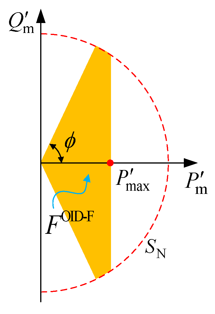
The PV array was connected to the grid by inverters, and it was assumed that its reactive power output was controlled by the mode of optimal inverter dispatch with a lower bound on the power factor (OID-F) [21], as shown in Figure 1.
Therefore, the reactive power provided by the PV generation to the grid was limited by its rated capacity and its active power, and the reactive power output could be written as Equation (3):
where represents the reactive power output of the PV, SN represents the rated capacity of the inverter, and represents the power factor angle of the PV.
2.2. Model of the Reactive Power Compensation Device
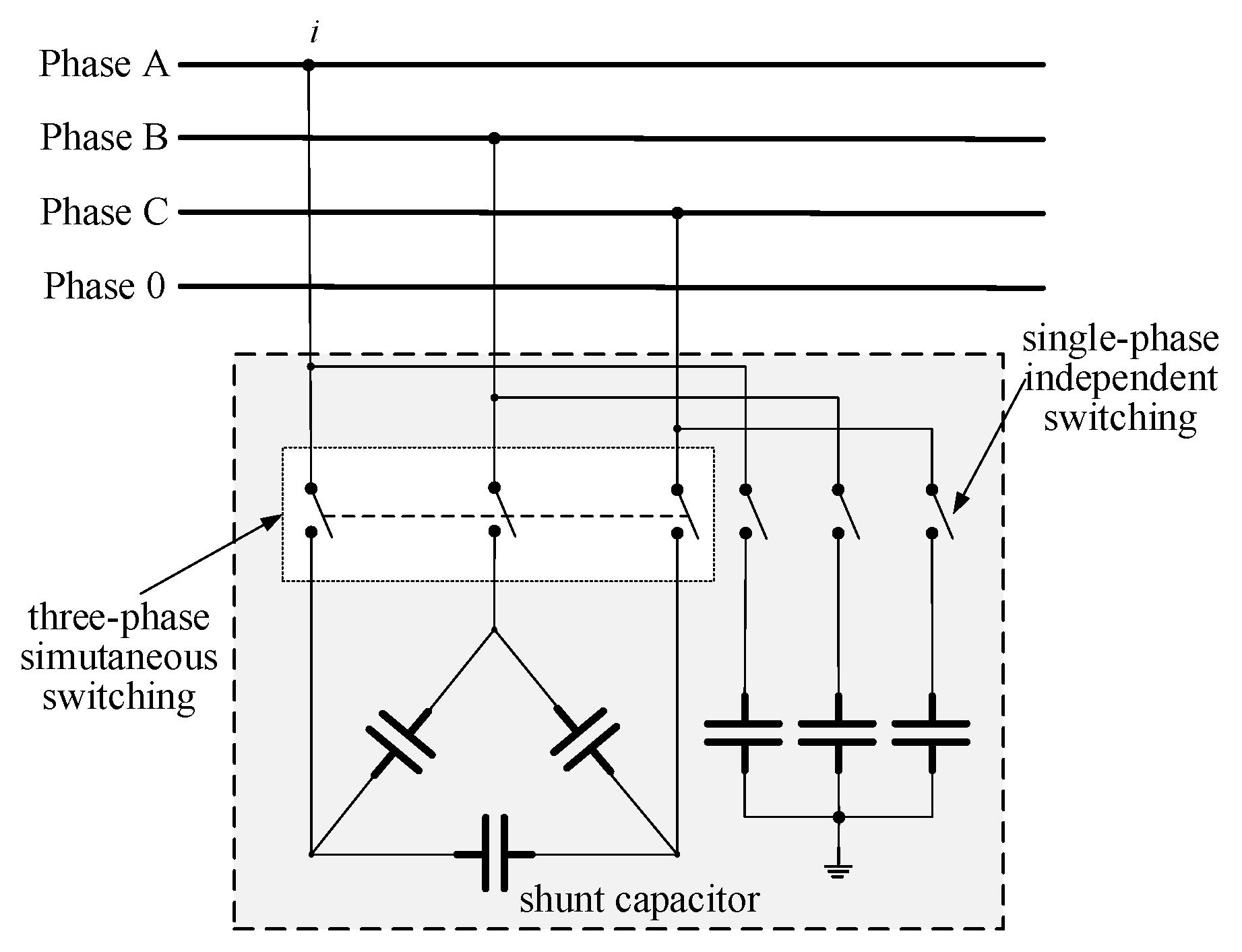
Capacitors are used as the RPC devices in LVDNs. The connection mode of these capacitors is shown in Figure 2. It includes the three-phase simultaneous switching capacity and the single-phase independent switching capacity. Because the RPC device contains single-phase independent switching capacity, it can improve the voltage quality problems under the three-phase unbalanced operation of LVDN. Two decision variables Qci,3 and Qci,ω are used to represent the three-phase simultaneous switching capacity and the single-phase independent switching capacity in the RPC device located in i-th bus, respectively.
2.3. Model of Feeder Line
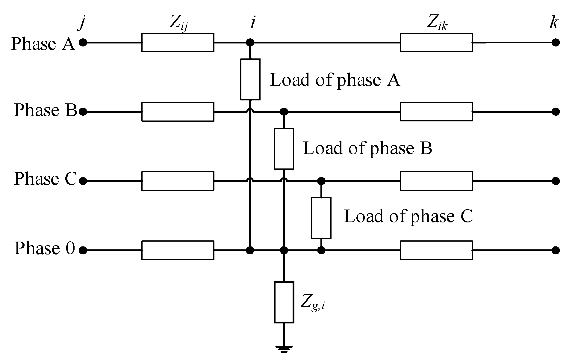
LVDNs usually adopt a three-phase four-wire radial network structure and form a return path through the neutral line. At the same time, in order to reduce the power loss and ground voltage when equipment fails, repetitive grounding of the neutral line is often used in LVDNs. Therefore, the equivalent circuit of a feeder line in a 380/220 V LVDN is shown in Figure 3. For ease of calculation, the mutual impedance and the ground branch admittance of the feeder lines are neglected, and the loads are connected between phases A/B/C and phase 0.
According to Kirchhoff’s Current Law, for the i-th bus, the power balance equation of phases A/B/C and the current balance equation of phase 0 flowing into the ground can be deduced, as shown in Equation (4):
where subscript ω denotes phases A, B, and C, and φli,ω represent the active power load and the power factor angle of phase ω of bus i, respectively, and Ppvi,ω and Qpvi,ω represent the active power and the reactive power of the PV generation of phase ω of bus i, respectively, that is, and in Equation (3). Qci,ω denotes the single-phase independent switching capacity of the RPC device in phase ω of bus i, which is a discrete variable, Qci,3 represents the three-phase simultaneous switching capacity of the RPC device in bus i, which is also a discrete variable, represents the voltage of phase ω of bus i, k∈i represents all buses k connected with bus i, and represents the voltage of phase 0 of bus i. Zki,ω denotes the impedance of phase ω of the line between bus k and bus i, and Zg,i denotes the grounding impedance of bus i.
2.4. Model of Distribution Transformer
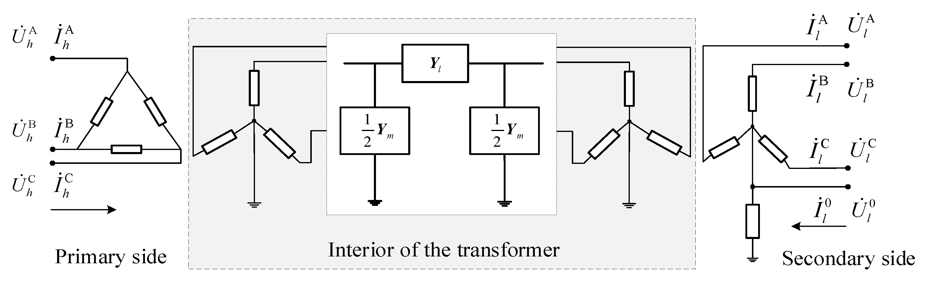
Since the actual three-phase four-wire LVDNs were usually in the asymmetry operation state, in order to obtain the operation state accurately, it was necessary to establish a detailed model of 10/0.4 kV three-phase distribution transformers. In reference [22], a three-phase transformer model based on the phase components method was proposed. The actual transformer was replaced by two ideal transformers that had high calculation accuracy, as shown in Figure 4.
For a three-phase double-winding transformer, the relationship between the voltage and injection current of two sides is shown in Equation (5):
where represents the vector of the injected current at the high-/low-voltage side, , , and represents the vector of the voltage at the high-/low-voltage side, , . The 6×6 matrix YT represents the admittance matrix consisting of the leakage admittance, whose element value can be obtained with the parameter yTsc that represents the admittance of the positive sequence short circuit test of the transformer, as shown in Equation (6). In this paper, yTsc = 1/(2+8×j), where j represents the imaginary number. N represents the connection matrix to describe the relationship between the internal voltage/current and the external voltage/current of the transformer. It is a constant matrix related to the connection group number of the three-phase transformer. Depending on whether a neutral point exists, N will be a 6×6, or 6×7, or 6×8 matrix. If the primary or secondary neutral point of the transformer does not exist, the corresponding column can be removed from the last two columns of the matrix N. It can be expressed as Equation (7). The superscript T of matrix N indicates the transposition of N:
where α and β represent the tap coefficients of the primary and secondary sides of the actual transformer, respectively, and 0 represents a 3×3 constant matrix with all the elements equal to 0. Both Cp and Cs are 3×3 constant matrices, which can be obtained from the connection group numbers of the two ideal three-phase transformers. Letting , then the element values in Cp and Cs can be obtained according to Table 1.
3. Robust Optimal Allocation Model for Decentralized RPC Devices
In the robust optimization problem, uncertain variables are described as the uncertain set. The optimization results of the decision variables can satisfy all the constraints when the uncertain variables are given as arbitrary values within their uncertain sets [23]. Robust optimization problems with uncertain variables can be described as shown in Equation (8):
where x represents the decision variables, ζ represents the uncertain variables, X is a set of decision variables, is a bounded set of uncertain variables, and sup (•) is an upper bound.
The optimal allocation of decentralized RPC devices for a three-phase four-wire LVDN takes into account the uncertainty of the PV output and the load power. The PV output is determined by the light intensity and temperature, so the uncertain variables include the load active power , the light intensity , and the temperature . Using the box uncertain set, the uncertain variables , and are expressed as the expected value and the disturbance, as , , . Based on the historical data of loads and the meteorological information of the area where the PV station is located, the expected values of the load power, the light intensity, the temperature, and their disturbance ranges can be determined. Then the upper and lower bounds of the variation range of the uncertain variables can be obtained. Therefore, the set of uncertain variables can be expressed as shown in Equation (9):
where C is the set of uncertain variables. / is the lower/upper bound of , / is the lower/upper bound of , and / is the lower/upper bound of .
3.1. Objective Function
To minimize the total active power loss of a LVDN, the objective function of the decentralized RPC optimal allocation model in a LVDN considering the uncertain fluctuation of the PV output and the load power is as follows:
where Ps,ω represents the injected active power of phase ω on the high-voltage side of the distribution transformer in the LVDN, U and θ represent the bus voltage amplitude and the phase angle, respectively, which are state variables. Qci,ω and Qci,3 are both the decision variables, npv represents the total number of PV generation buses, and nl represents the total number of load buses. The total network loss is equal to the sum of the injected active power on the high-voltage side of the distribution transformer and the total PV power outputs minus the total active power loads.
3.2. Constraints
(1) Power balance equation
The power balance equation of a three-phase four-wire LVDN with distributed PV integration includes the power balance equation of each bus in the feeders and the equation of the relationship between the voltage and the current of the distribution transformer, as shown in Equations (4) and (5).
(2) Voltage deviation limit constraints
To ensure that the users are supplied with qualified electric energy, the optimal RPC allocation should ensure that the voltage deviation of each bus in the LVDN does not exceed the security limit no matter how the light intensity, temperature, and load power change in their own fluctuation interval, as shown in Equation (11):
where and represent the lower and upper limits of the voltage amplitude of phase ω in bus i, respectively.
(3) Voltage unbalance factor limit constraints
The degree of unbalance of the three-phase voltage is an important index of voltage quality in the LVDN. Excessive three-phase unbalance of the voltage will be harmful to the normal operation of power equipment such as transformers. Therefore, the three-phase unbalance constraints of the bus voltage should be considered in the RPC optimal allocation problem of the LVDN to keep it within the secure operation range. In this paper, the VUF defined by the International Electrotechnical Commission (IEC) is used to describe the unbalance degree of the three-phase voltage of each bus, as shown in Equation (12). In accordance with the IEC 61000-3-13 standard, the maximum VUF during normal operation in power systems must not exceed 2% [24]:
where εi represents the VUF of bus i and εmax represents the maximum VUF during normal operation, with a value of 2%. and represent the root mean square (RMS) value of the negative sequence component and the RMS value of the positive sequence component of the three-phase voltage of bus i, respectively, which can be computed by the symmetric components method, as shown in Equation (13):
where the constant complex number a=e j120°.
(4) Reactive Power Output of the PV Constraints
where Spvi,ωN and represent the rated capacity and the power factor angle of the PV generation in phase ω of bus i.
(5) Switching capacity of the constraints of RPC devices
Because capacitors in the RPC devices are switched on or off in groups, their switching capacities are discrete variables. The constraints of Qci,3 and Qci,ω are shown in Equations (15) and (16), respectively:
where Nτ and Nπ represent the total number of integer values of Qci,3 and Qci,ω, respectively. qcτ and qcπ represent the τ-th and π-th integer values of Qci,3 and Qci,ω, respectively. σi,τ and σi,ω,π represent the switching states of the τ-th and π-th group capacitors in the i-th RPC device, respectively. They are discrete decision variables that only take the values of 0 or 1. When the value is 0, it denotes that the integer value qcτ /qcπ is not selected, and when the value is 1, it denotes that the integer value qcτ /qcπ is selected. It can be seen that Qci,3 can be expressed as the linear combination of its Nτ integer values, and Qci,ω can be expressed as the linear combination of its Nπ integer values.
4. Solution of Robust RPC Optimization Model
The robust optimal allocation model of decentralized RPC devices in a three-phase four-wire LVDN that is composed of formulas (10)−(16) is a nonlinear programming problem with discrete variables and uncertain variables. Determining how to deal with the discrete variables and the uncertain variables is the key problem in solving the optimization model.
4.1. Addressing the Discrete Variables Problem
The convex relaxation and introducing penalty function methods are used to deal with the discrete variables [25]. First, σi,τ and σi,ω,π are relaxed to be continuous variables whose values are between 0 and 1, that is, the second formulas in Equations (15) and (16) are relaxed into Equations (17) and (18), respectively. The penalty functions are added to the original objective function to force σi,τ and σi,ω,π to be near the integer values. The objective function after adding the penalty functions is shown in Equation (19):
where f (•) represents the original objective function, ρ is the penalty factor of the penalty functions, and R is the total number of candidate installation buses for the RPC devices. It can be seen that when the values of σi,τ and σi,ω,π are 0 or 1, F in Equation (19) is equal to the original objective function f.
4.2. Bi-Level Optimization Method
The robust optimization theory is a powerful tool for solving optimization problems with uncertain variables. It obtains the optimal scheme that can satisfy all the constraints under all the scenarios of the uncertain variables that vary in their fluctuation range. Simply by solving the optimization model under the extreme scenarios, the obtained optimal scheme can satisfy all the constraints under any scenario of uncertain variables in their uncertain sets. Therefore, the key problems for solving the above robust optimal allocation model of decentralized RPC devices in a LVDN are as follows:
Determining how to search two scenarios of uncertain variables in their uncertain sets, which correspond to the highest and lowest bus voltage level in the operation of the LVDN;
Determining how to search the decision variables in the feasible region of the robust optimization model that can satisfy all the constraints in the above two extreme scenarios.
To solve these key problems accurately and effectively, the above robust optimization model can be transformed into bi-level deterministic optimization models [26]:
(1) Upper-level optimization model
The upper level optimization model is designed to accurately determine the decision variables in the feasible region that can minimize the objective function under the premise of satisfying all the constraints in the two extreme scenarios of uncertain variables, as shown in Equation (20):
where the indicators H and L represent the variables that correspond to extreme scenarios of the highest and lowest bus voltages, respectively. and represent the probability of the highest voltage extreme scenario and the lowest voltage extreme scenario, respectively, and the values of both are 1/2. Equations hH(•) and hL(•) represent the power balance equations of each bus that correspond to the highest and lowest bus voltage extreme scenarios, respectively. CH represents the values of uncertain variables in the extreme scenario of the highest bus voltage level, CL represents the values of uncertain variables in the extreme scenario of the lowest bus voltage level, and the equation UH,n,ω=UL,n,ω represents the fact that the voltage of the slack bus remains equal in the two extreme scenarios.
By solving the deterministic upper level optimization model (20), the decision variables σi,τ and σi,ω,π that can satisfy all the constraints in the two extreme scenarios of the uncertain variables can be obtained. Then the decision variables Qci,3 and Qci,ω can also be obtained according to Equations (15) and (16).
(2) Lower-level optimization model
To search the uncertain variables CH and CL that correspond to the two extreme scenarios, two deterministic lower level optimization models are established, and the objective functions are the sum of the phase A/B/C voltages of the bus corresponding to the highest and lowest voltage in the LVDN. Assuming that the voltage of bus t is the highest in the LVDN, the lower level optimization model for determining the uncertain variables CH that correspond to the extreme scenario with the highest voltage level is shown in Equation (21):
where UH,t,ω represents the highest voltage level in phase ω of bus t.
Similarly, assuming that the voltage of bus u is the lowest in the LVDN, the lower level optimization model for determining the uncertain variables CL that correspond to the extreme scenario with the lowest voltage level is solved as shown in Equation (22):
where UL,u,ω represents the lowest voltage level in phase ω of bus u.
When the decentralized RPC scheme Qci,3 and Qci,ω is determined, the uncertain variables CH that correspond to the extreme scenarios with the highest voltage level can be obtained by solving the deterministic lower level optimization model (21), and the uncertain variables CL that correspond to the extreme scenarios with the lowest voltage level can also be obtained by solving the deterministic lower level optimization model (22).
By solving the upper level optimization model (20) and the two lower level optimization models (21) and (22) iteratively, the robust optimal allocation scheme of the decentralized RPC devices that can satisfy all the constraints under any scenario of uncertain variables in their uncertain sets can be obtained. The bus voltage level and the other operation parameters in the two extreme scenarios can also be obtained.
4.3. Calculation Steps
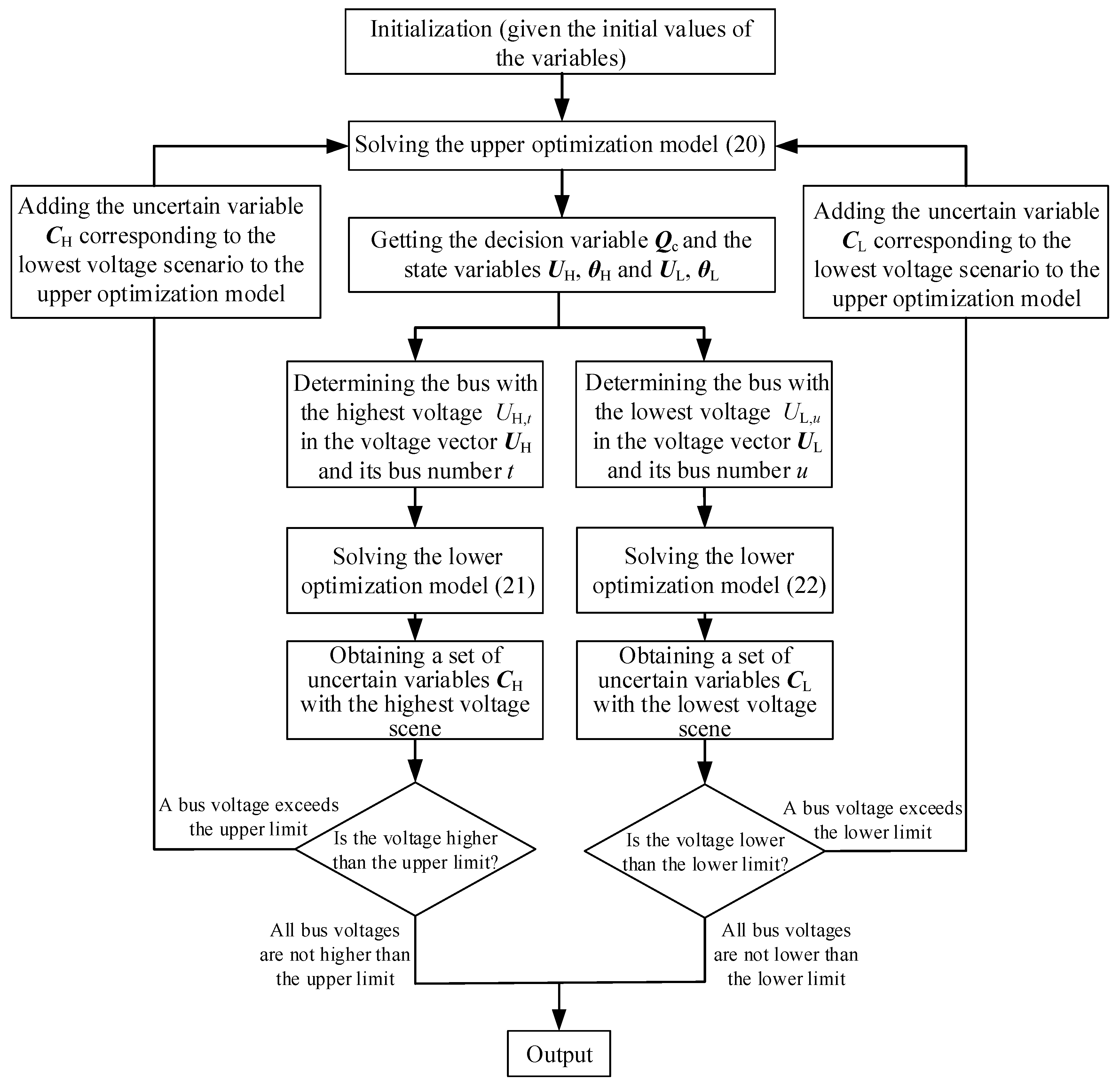
The flowchart of the bi-level optimization method for solving the robust optimal allocation model of decentralized RPC devices in a three-phase four-wire LVDN is shown in Figure 5.
The solution steps are as follows:
Give the system parameters and initialize the variables. Assume that the initial values of the uncertain variables in the two extreme scenarios CH and CL are both equal to the expected values T0, S0 and Pl0;
By solving the upper level optimization model (20), the decision variables Qci,3 and Qci,ω and the state variables UH, θH and UL, θL are obtained;
Determine the highest voltage UH,t and the corresponding bus number t in the voltage vector UH. Solve the lower level optimization model (21) to obtain the uncertain variables CH of the highest voltage scenario in the fluctuation range of uncertain variables;
Determine the lowest voltage UL,u and the corresponding bus number u in the voltage vector UL. Solve the lower level optimization model (22) to obtain the uncertain variables CL of the lowest voltage scenario in the fluctuation range of uncertain variables;
Determine whether the bus voltage UH,t,ω in the highest voltage scenario is higher than the upper limit . At the same time, determine whether the bus voltage UL,u,ω in the lowest voltage scenario is lower than the lower limit ;
If all the bus voltages do not exceed the security limits, the output result of Qci,3 and Qci,ω is obtained. If there is a bus voltage that exceeds the security limit, add the uncertain variables CH and CL that correspond to the two extreme scenarios obtained from Steps (3) and (4) to the upper level optimization model, and return to Step (2).
5. Case Study
5.1. Parameters of the LVDN and the Power Flow Calculation Result
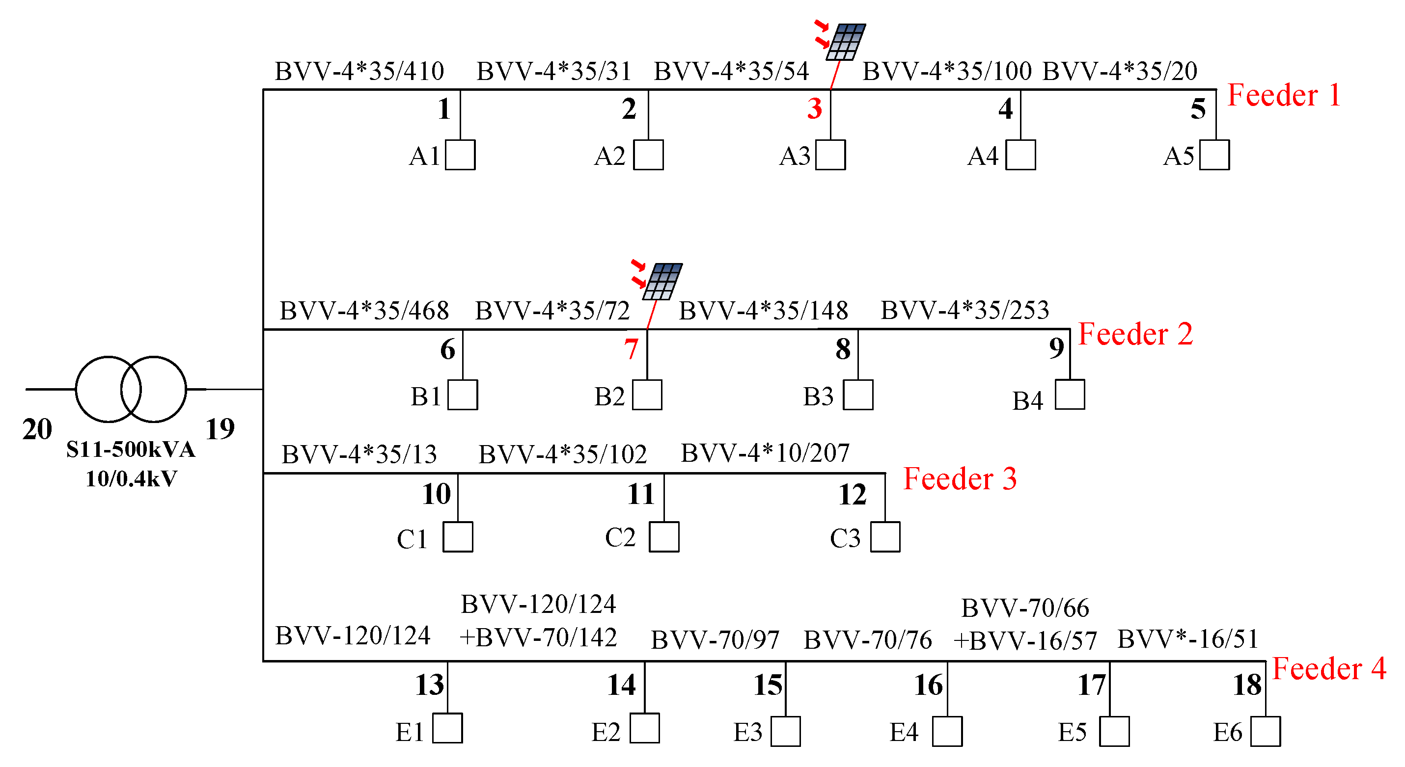
To verify the correctness of the robust optimal allocation method of decentralized RPC devices in a three-phase four-wire LVDN, an actual three-phase four-wire LVDN was taken as a test example. The network topology diagram of the LVDN is shown in Figure 6. The distribution transformer was a S11-500 type and its rated capacity was 500 kVA. The connection group number of the three-phase transformer was Dyn11, and the ratio was 10/0.4 kV. The singe phase parameters of each branch in the LVDN are shown in Table 2.
The resistance and reactance of each phase in a branch are the same. A three-phase grid-connected PV station was connected to bus 3 with a rated capacity of 10 kVA, and a single-phase grid-connected PV station was connected to bus 7 with rated capacity of 4 kVA. The predicted power of each phase of the load is shown in Table 3. It was assumed that the relative prediction error of the active power load in each bus was –10% ~ +10%, and the power factor remained unchanged. According to the historical short-term light intensity and the temperature changing curve of the region, it was also assumed that the fluctuation range of temperature was 20°C ~ 30°C, and the fluctuation range of light intensity was 900 W/m2 ~ 1100 W/m2. The upper and lower bounds of the voltage amplitudes of the A/B/C phases were –10% and +7% of the rated voltage, respectively. The deterministic upper and lower level optimization models were solved by the nonlinear programming solver IPOPT in the mature commercial software GAMS [27].
Bus 20 was selected as the slack bus whose line voltage amplitude was 10.3 kV, and the voltage angles of the A/B/C phases were given as 0, –120°, and 120°, respectively. It was assumed that the expected value of the local light intensity was S = 1000 W/m2, the expected value of the temperature was T = 25°C, and the expected value of the load power is shown in Table 3. The results of the power flow calculation in the LVDN under the expected scenario of the uncertain variables are shown in Table 4.
From Table 4, it can be seen that the voltage deviation of many buses at the end of the feeders in the LVDN (e.g., buses 4, 5, 8, 9, 17, and 18) exceeded –10% (the voltage was lower than 198 V), and the VUF of buses 4, 5 and 9 exceeded 2%. Therefore, for the LVDN, the three-phase unbalance degree was relatively high, and there were serious low-voltage problems, which would affect the normal power consumption of users. The total network loss was 44.159 kW, accounting for 18.66% of the total load of the LVDN, which was relatively large.
5.2. Robust Optimal Allocation of Decentralized RPC Devices
In the optimal allocation model of decentralized RPC devices, the lower and upper bounds of the voltage of each bus in the LVDN were set, as shown in Table 5. The set parameters of the capacities of the decentralized RPC devices are shown in Table 6. When the uncertainty of the PV output and the load power were not considered, for example, when the light intensity, temperature, and load of each bus were the expected values and all the load buses were taken as the candidate decentralized RPC positions, after solving the deterministic optimal allocation model of decentralized RPC devices, the obtained decentralized RPC capacity is shown in Table 7. It can be seen from Table 7 that bus 10 needed to have a single-phase independent switching RPC device installed whose capacities in phases B and C were both 20 kvar. Buses 5, 9, and 18 needed to have three-phase simultaneous switching RPC devices with the capacities of 30 kvar, 10 kvar, and 10 kvar installed, respectively (the RPC capacities in the other load buses were all 0, which is not listed in Table 7). In addition, the values in the parentheses are the optimal calculation results of solving the optimization model with relaxation of the discrete variables to the continual variables. It can be seen that the optimal calculation results of the discrete variables were near their integer values. Therefore, the proposed methods of convex relaxation and introducing penalty function that were used to address the discrete variables problem were effective.
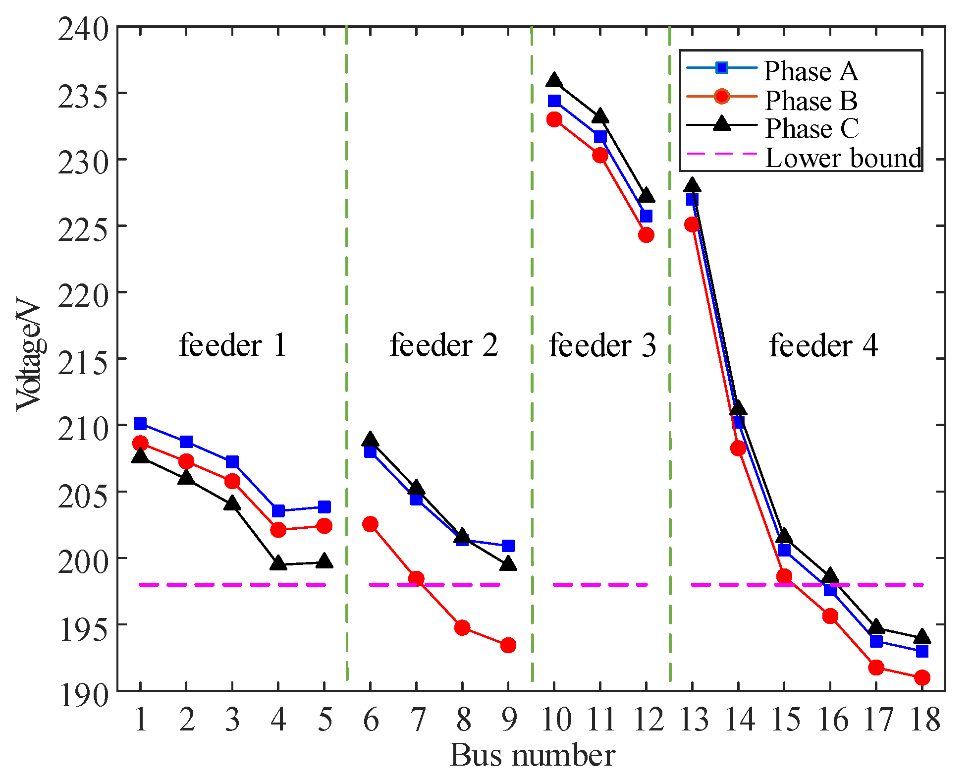
After the installation and operation of the decentralized RPC devices corresponding to the deterministic optimization, and under the expected value of uncertain variables, the voltage deviation and the VUF of each bus in the LVDN were all within the security operation limit, which significantly improved the voltage quality. The total network loss of the LVDN was 30.597 kW, which accounted for 12.93% of the total load. Hence, the total network loss was obviously reduced. However, for the situation when the actual load of each bus was 10% larger than the expected value, the light intensity was 900 W/m2, and the temperature was 30°C, the voltage of each bus under the deterministic decentralized RPC scheme is shown in Figure 7. It can be seen that the voltage amplitudes of the B phases of buses 8 and 9 are 194.754 V and 193.428 V, respectively, which are clearly lower than the lower bound of the secure operation limit (198 V). Moreover, the voltage amplitudes of the A/B/C phases of buses 17 and 18, and the voltage amplitudes of phases A/B of bus 16 were also lower than the lower bound of the secure operation limit (198 V). These low-voltage buses would affect the secure operation of the power equipment and the secure power consumption of users integrated in the buses. Therefore, although the deterministic decentralized RPC scheme could improve the voltage quality, its robustness was poor. When the load power and the PV output fluctuated, some bus voltages would exceed the secure operation limit.
To improve the robustness of the decentralized RPC scheme and improve the quality of voltage in the LVDN, we further considered the uncertain fluctuation of the load power and the PV output for the optimization calculation. The upper and lower level optimization models converged after three alternative iterations. The obtained robust decentralized RPC scheme is shown in Table 8. It can be seen from Table 8 that bus 9 needed to have a three-phase simultaneous switching RPC device with a capacity of 15 kvar installed. It can also be seen that phase A of bus 4, phases A and C of bus 5, phases A and B of bus 15, phases A and C of bus 16, and phase C of bus 17 needed to have single-phase independent switching RPC devices with the capacities of 20 kvar, 10 kvar and 20 kvar, 5 kvar and 20 kvar, 15 kvar and 10 kvar, 10 kvar installed, respectively (the RPC capacity in other load buses are all 0, which is not listed in Table 8). Compared to Table 7, only bus 9 had a three-phase simultaneous switching RPC device installed and more single-phase independent switching RPC devices were installed in the A/B/C phases, which could more effectively solve the three-phase imbalance problem under uncertain fluctuations of the load power and the PV output.
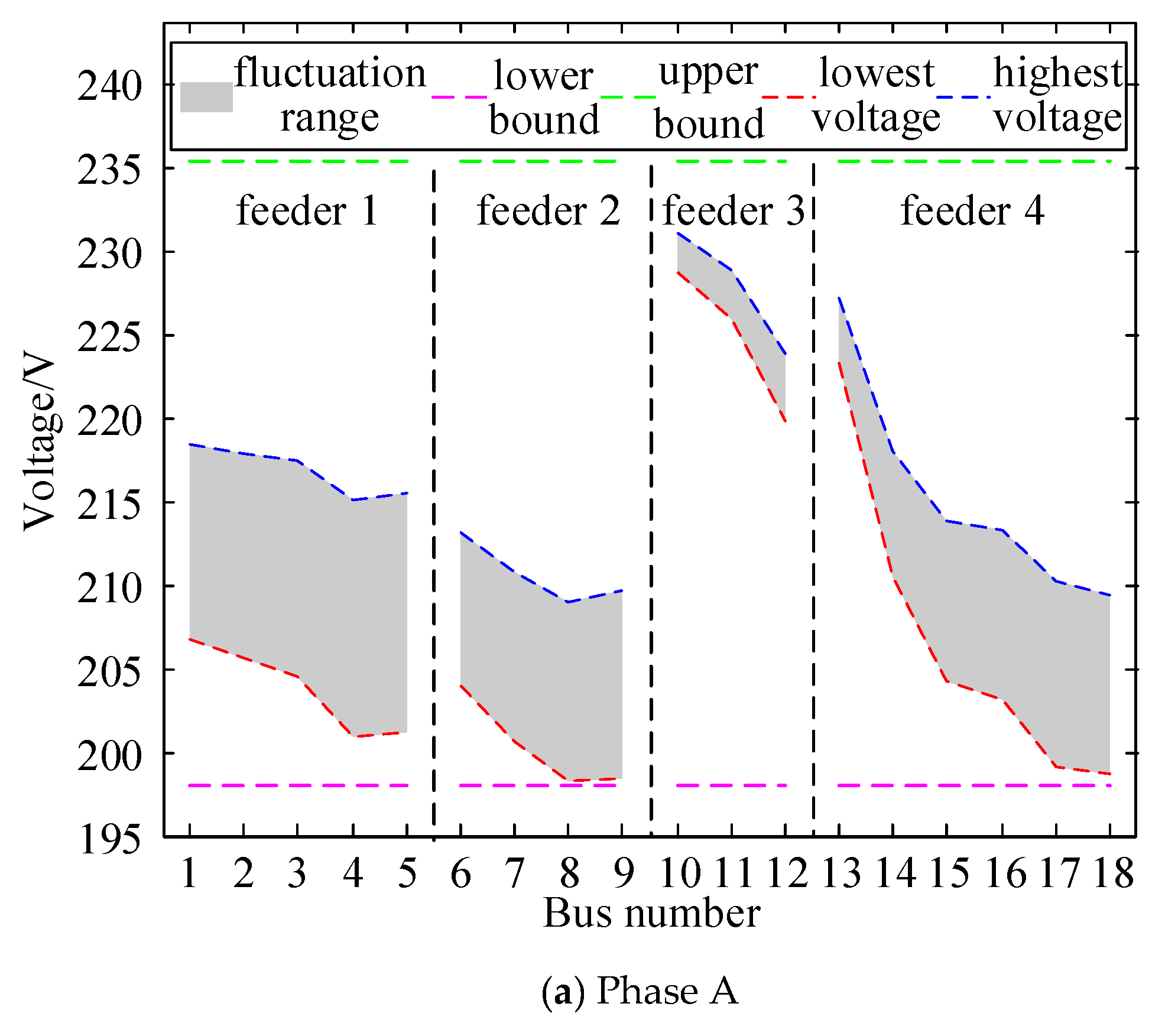
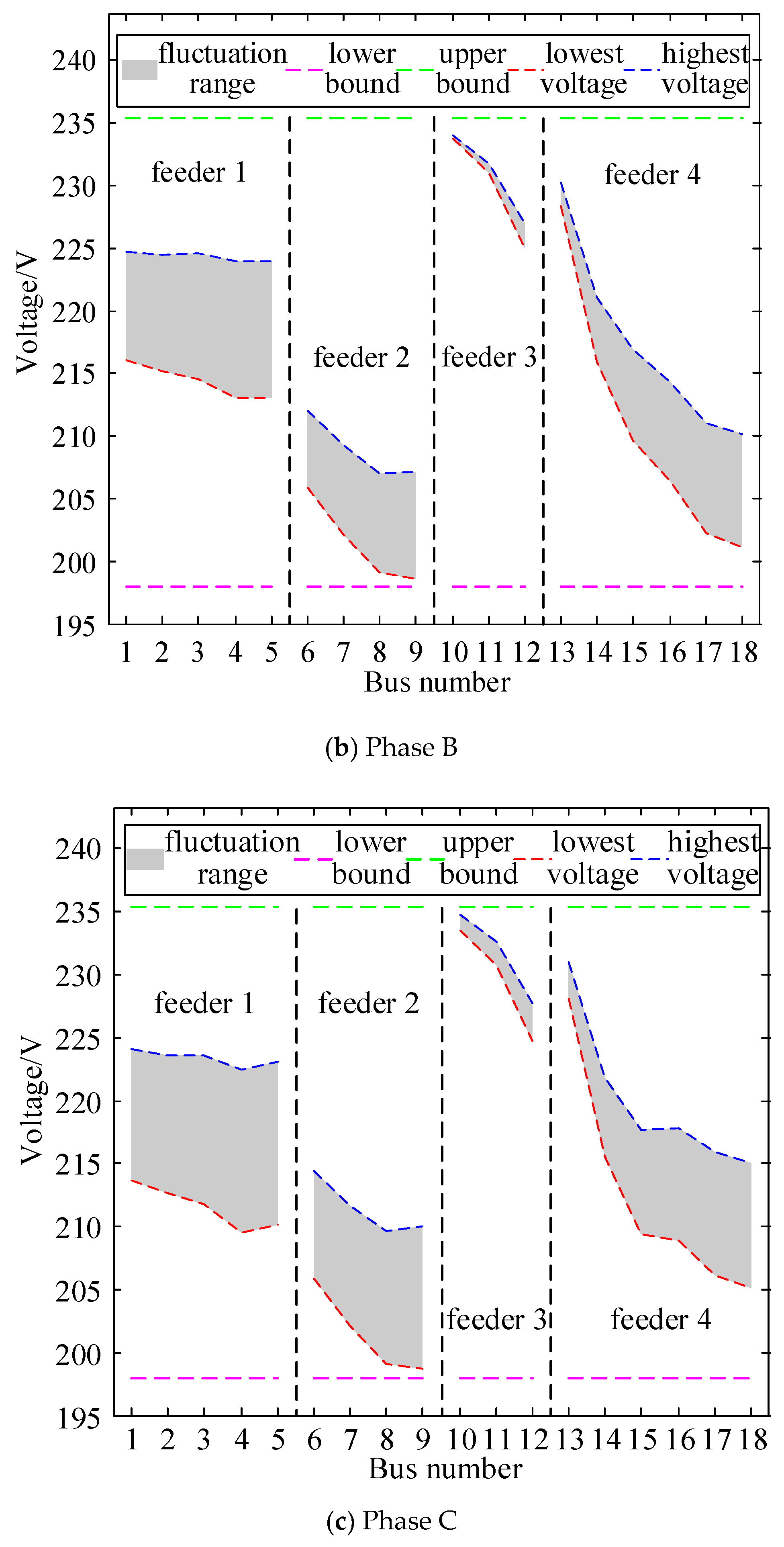
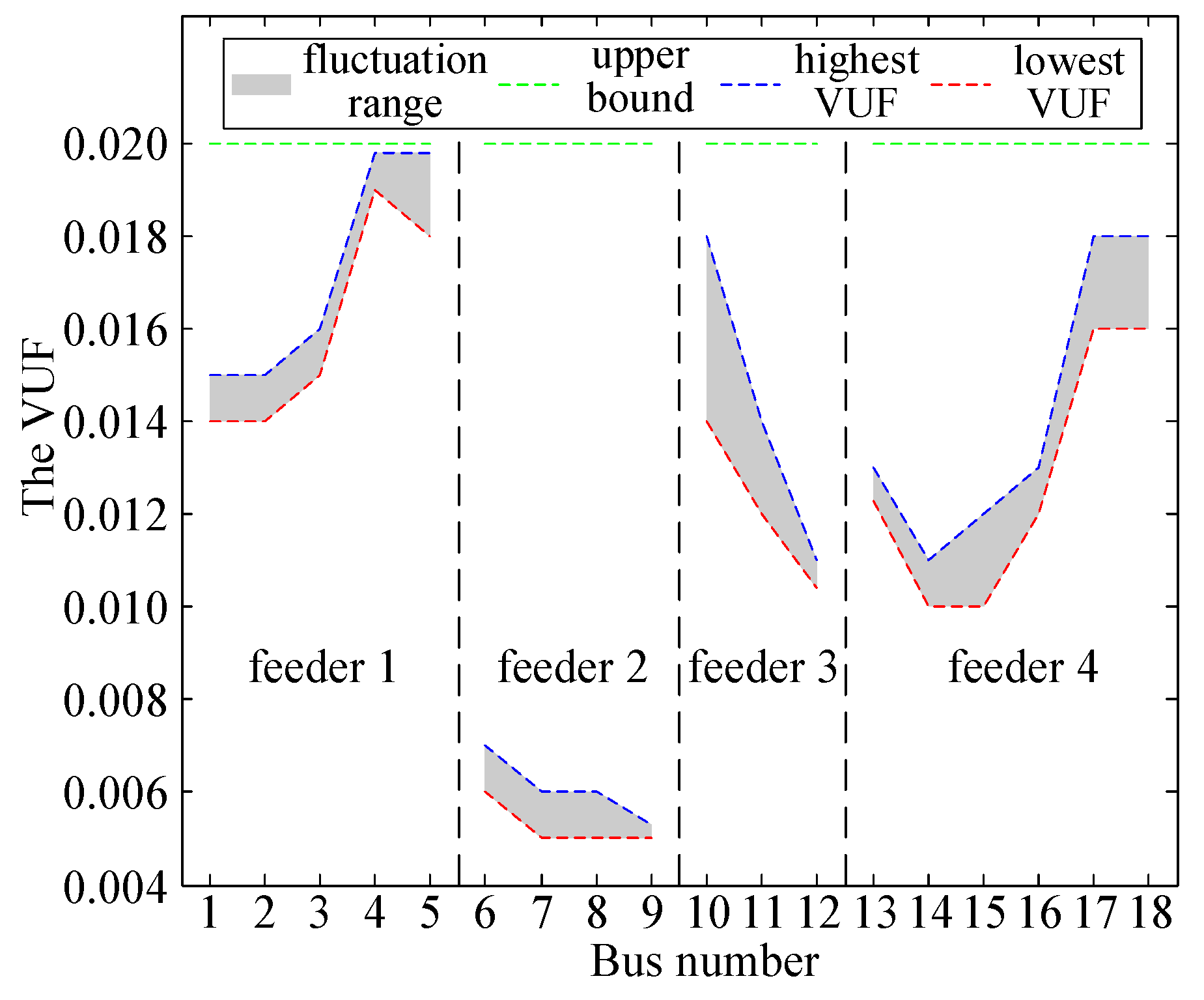
After the robust decentralized RPC scheme, for the situation when the uncertain variables fluctuated as arbitrary scenarios within their uncertain sets, the voltage fluctuation range of the A/B/C phases of each bus are shown in Figure 8, and the fluctuation range of VUF of each bus is shown in Figure 9. As can be seen from Figure 8 and Figure 9, the robust decentralized RPC scheme in Table 8 could ensure that the voltage deviation and the VUF of all the buses in the LVDN were within the qualified fluctuation range when the light intensity, temperature, and bus load changed arbitrarily within their uncertain sets, and the scheme had good robustness. Moreover, after the robust decentralized RPC scheme, the network loss of the LVDN also decreased. When the extreme scenario of the lowest voltage occurred, the total network loss decreased to 27.669 kW, which accounted for 10.60% of the total load. When the extreme scenario of the highest voltage occurred, the total network loss decreased to 15.826 kW, which accounted for 7.40% of the total load. In the expected scenario, the total network loss decreased to 21.872 kW, which accounted for 9.24% of the total load. Compared with the deterministic decentralized RPC scheme without consideration of the fluctuation of the uncertain variables, the obtained robust decentralized RPC scheme not only enhanced the robustness of the operation of the LVDN under the uncertain fluctuations of the PV output and the load power, but also reduced the total network loss. Therefore, the obtained robust decentralized RPC scheme is more suitable for practical engineering application.
6. Conclusions
In this study, to address the voltage quality problems caused by three-phase unbalanced load power, single-phase PV integration, and the uncertainties of the PV output and the load power in three-phase four-wire LVDNs, a robust optimal allocation of decentralized RPC devices model for a three-phase four-wire LVDN with consideration of the uncertainties of the PV output and the load power is established. Discrete variables for the RPC capacity in the model were addressed with the convex relaxation technique and the adding penalty functions in the objective function, and a bi-level optimization method was adopted to solve the robust optimal allocation model. The test results for an actual three-phase four-wire LVDN showed that the decentralized RPC scheme obtained by solving the proposed robust optimization model can satisfy the requirements of all bus voltages within the qualified range when the PV output and the bus load power change arbitrarily within their uncertain sets. At the same time, the total network loss is significantly reduced from 44.159 kW (18.66%) to 21.872 kW (9.24%) after installing the RPC devices in the expected scenario. In the extreme scenario of the lowest voltage and the highest voltage, the total network loss decreased to 27.669 kW (10.60%) and 15.826 kW (7.40%), respectively. The optimal allocation scheme has good robustness and economic benefit, and it is suitable for practical engineering applications. There are always R > X for the feeders in LVDNs, thus installing energy storage devices is another effective way to improve voltage quality, therefore, how to coordinate the energy storage devices and the RPC devices to improve voltage quality in LVDNs is a possible direction for future research.
Author Contributions
Formal analysis, S.H.; Investigation, Z.T., H.J. and Y.S.; Methodology, Shunjiang Lin, S.H. and H.Z.; Supervision, S.L. and M.L.; Writing—review & editing, S.H.
Funding
This research was funded by the National Basic Research Program of China (973 Program) (grant no. 2013CB228205), the National Natural Science Foundation of China (grant no. 51207056).
Acknowledgments
The authors gratefully acknowledge the support of the National Basic Research Program of China and the National Natural Science Foundation of China.
Conflicts of Interest
The authors declare no conflict of interest.
References
Hishikawa, Y.; Doi, T.; Higa, M.; Yamagoe, K.; Ohshima, H.; Takenouchi, T.; Yoshita, M. Voltage-dependent temperature coefficient of the I–V curves of crystalline silicon photovoltaic modules. IEEE J. Photovolt.2018, 8, 48–53. [Google Scholar] [CrossRef]
Kumar, M.; Kumar, A. Performance assessment of different photovoltaic technologies for canal-top and reservoir applications in subtropical humid climate. IEEE J. Photovolt.2019, 9, 722–732. [Google Scholar] [CrossRef]
Chou, J.; Kuo, C.; Kuo, P.; Lai, C.; Nien, Y.; Liao, Y.; Ko, C.; Yang, C.; Wu, C. The retardation structure for improvement of photovoltaic performances of dye-sensitized solar cell under low illumination. IEEE J. Photovolt.2019, 9, 926–933. [Google Scholar] [CrossRef]
Kim, J.J.; Choi, J.H.; Park, S.Y.; Bhang, B.G.; Nam, W.J.; Cha, H.L.; Park, N.; Ahn, H. Prediction model for PV performance with correlation analysis of environmental variables. IEEE J. Photovolt.2019, 9, 832–841. [Google Scholar] [CrossRef]
Su, X.; Masoum, M.A.S.; Wolfs, P.J. Optimal PV inverter reactive power control and real power curtailment to improve performance of unbalanced four-wire LV distribution networks. IEEE Trans. Sustain. Energy2014, 5, 967–977. [Google Scholar] [CrossRef]
Araujo, L.R.; Penido, D.R.R.; Jr, S.C.; Pereira, J.L.R.A. Three-Phase optimal power-flow algorithm to mitigate voltage unbalance. IEEE Trans. Power Deliv.2013, 28, 2394–2402. [Google Scholar] [CrossRef]
Robbins, B.A.; Dominguez-Garcia, A.D. Optimal reactive power dispatch for voltage regulation in unbalanced distribution systems. IEEE Trans. Power Syst.2016, 31, 1–11. [Google Scholar] [CrossRef]
Tian, Z.; Wu, W.; Zhang, B.; Bose, A. Mixed-integer second-order cone programing model for var optimisation and network reconfiguration in active distribution networks. IET Gener. Transm. Distrib.2016, 10, 1938–1946. [Google Scholar] [CrossRef]
Jabr, R.A. Minimum loss operation of distribution networks with photovoltaic generation. IET Renew. Power Gener.2014, 8, 33–44. [Google Scholar] [CrossRef]
He, Y.; Gao, S.; Lu, S.; Zhao, X.; Han, H. Reactive power optimization of distribution network including photovoltaic power considering harmonic factors. In Proceedings of the 2016 China International Conference on Electricity Distribution (CICED’16), Xi’an, China, 10–13 August 2016; pp. 1–7. [Google Scholar]
Farivar, M.; Neal, R.; Clarke, C.; Low, S. Optimal inverter VAR control in distribution systems with high PV penetration. In Proceedings of the 2012 IEEE Power and Energy Society General Meeting(PES’12), San Diego, CA, USA, 22–26 July 2012; pp. 1–7. [Google Scholar]
Li, H.; Liu, S.; Lu, S.; Chen, L.; Yuan, X.; Huang, J. Reactive power optimization of distribution network including photovoltaic power and SVG considering harmonic factors. In Proceedings of the 2017 International Conference on High Voltage Engineering and Power Systems(ICHVEPS’17), Bali, Indonesia, 2–5 October 2017; pp. 219–224. [Google Scholar]
Mostafa, H.A.; El-Shatshat, R.; Salama, M.M.A. Multi-objective opimization for the operation of an electric distribution system with a large number of single phase solar generators. IEEE Trans. Smart Grid2013, 4, 1038–1047. [Google Scholar] [CrossRef]
Hu, J.; Marinelli, M.; Coppo, M.; Zecchino, A.; Bindner, H.W. Coordinated voltage control of a decoupled three-phase on-load tap changer transformer and photovoltaic inverters for managing unbalanced networks. Electr. Power Syst. Res.2016, 131, 264–274. [Google Scholar] [CrossRef]
Chen, T.-H.; Yang, W.-C. Analysis of multi grounded four-wire distribution systems considering the neutral grounding. IEEE Trans. Power Deliv.2001, 16, 710–717. [Google Scholar] [CrossRef]
Antonio Padilha Feltrin, R.M.C.; Ochoa, L.F. Power flow in four-wire distribution networks-general approach. IEEE Trans. Power Syst.2003, 18, 1283–1290. [Google Scholar]
Alam, M.J.E.; Muttaqi, K.M.; Sutanto, D. A three-phase power flow approach for integrated 3-wire mv and 4-wire multigrounded lv networks with rooftop solar pv. IEEE Trans. Power Syst.2013, 28, 1728–1737. [Google Scholar] [CrossRef]
Wolfs, P.; Masoum, M.A.S.; Su, X. Comprehensive optimal photovoltaic inverter control strategy in unbalanced three-phase four-wire low voltage distribution networks. IET Gener. Transm. Distrib.2014, 8, 1848–1859. [Google Scholar]
Zeraati, M.; Golshan, M.E.H.; Guerrero, J.M. Voltage quality improvement in low voltage distribution networks using reactive power capability of single-phase PV inverters. IEEE Trans. Smart Grid2018, 1. [Google Scholar] [CrossRef]
Coelho, R.F.; Cancer, F.; Martins, D.C. A proposed photovoltaic module and array mathematical modeling destined to simulation. In Proceedings of the IEEE International Symposium on Industrial Electronic (ISIE’09), Seoul, Korea, 5–8 July 2009; pp. 1624–1629. [Google Scholar]
Ding, T.; Li, C.; Yang, Y.; Jiang, J.; Bie, Z.; Blaabjerg, F. A two-stage robust optimization for centralized-optimal dispatch of photovoltaic inverters in active distribution networks. IEEE Trans. Sustain. Energy2017, 8, 744–754. [Google Scholar] [CrossRef]
Moorthy, S.S.; Hoadley, D. A new phase-coordinate transformer model for ybus analysis. IEEE Trans. Power Syst.2002, 17, 951–956. [Google Scholar] [CrossRef]
Ben-Tal, A.; Nemirovski, A. Robust optimization methodology and applications. Math. Program.2002, 92, 453–480. [Google Scholar] [CrossRef]
Rodríguez, A.; Bueno, E.J.; Mayor, Á.; Rodríguez, F.J.; García-Cerrada, A. Voltage support provided by STATCOM in unbalanced power systems. Energies2014, 7, 1003–1026. [Google Scholar] [CrossRef]
Logist, F.; Sager, S.; Kirches, C.; Van Impe, J.F. Efficient multiple objective optimal control of dynamic systems with integer controls. J. Process Control2010, 20, 810–822. [Google Scholar] [CrossRef]
Lin, S.; He, S.; Zhang, H.; Liu, M.; Tang, Z.; Jiang, H.; Song, Y.
Robust Optimal Allocation of Decentralized Reactive Power Compensation in Three-Phase Four-Wire Low-Voltage Distribution Networks Considering the Uncertainty of Photovoltaic Generation. Energies2019, 12, 2479.
https://doi.org/10.3390/en12132479
AMA Style
Lin S, He S, Zhang H, Liu M, Tang Z, Jiang H, Song Y.
Robust Optimal Allocation of Decentralized Reactive Power Compensation in Three-Phase Four-Wire Low-Voltage Distribution Networks Considering the Uncertainty of Photovoltaic Generation. Energies. 2019; 12(13):2479.
https://doi.org/10.3390/en12132479
Chicago/Turabian Style
Lin, Shunjiang, Sen He, Haipeng Zhang, Mingbo Liu, Zhiqiang Tang, Hao Jiang, and Yunong Song.
2019. "Robust Optimal Allocation of Decentralized Reactive Power Compensation in Three-Phase Four-Wire Low-Voltage Distribution Networks Considering the Uncertainty of Photovoltaic Generation" Energies 12, no. 13: 2479.
https://doi.org/10.3390/en12132479
APA Style
Lin, S., He, S., Zhang, H., Liu, M., Tang, Z., Jiang, H., & Song, Y.
(2019). Robust Optimal Allocation of Decentralized Reactive Power Compensation in Three-Phase Four-Wire Low-Voltage Distribution Networks Considering the Uncertainty of Photovoltaic Generation. Energies, 12(13), 2479.
https://doi.org/10.3390/en12132479
Note that from the first issue of 2016, this journal uses article numbers instead of page numbers. See further details here.
Article Metrics
No
No
Article Access Statistics
For more information on the journal statistics, click here.
Multiple requests from the same IP address are counted as one view.
Lin, S.; He, S.; Zhang, H.; Liu, M.; Tang, Z.; Jiang, H.; Song, Y.
Robust Optimal Allocation of Decentralized Reactive Power Compensation in Three-Phase Four-Wire Low-Voltage Distribution Networks Considering the Uncertainty of Photovoltaic Generation. Energies2019, 12, 2479.
https://doi.org/10.3390/en12132479
AMA Style
Lin S, He S, Zhang H, Liu M, Tang Z, Jiang H, Song Y.
Robust Optimal Allocation of Decentralized Reactive Power Compensation in Three-Phase Four-Wire Low-Voltage Distribution Networks Considering the Uncertainty of Photovoltaic Generation. Energies. 2019; 12(13):2479.
https://doi.org/10.3390/en12132479
Chicago/Turabian Style
Lin, Shunjiang, Sen He, Haipeng Zhang, Mingbo Liu, Zhiqiang Tang, Hao Jiang, and Yunong Song.
2019. "Robust Optimal Allocation of Decentralized Reactive Power Compensation in Three-Phase Four-Wire Low-Voltage Distribution Networks Considering the Uncertainty of Photovoltaic Generation" Energies 12, no. 13: 2479.
https://doi.org/10.3390/en12132479
APA Style
Lin, S., He, S., Zhang, H., Liu, M., Tang, Z., Jiang, H., & Song, Y.
(2019). Robust Optimal Allocation of Decentralized Reactive Power Compensation in Three-Phase Four-Wire Low-Voltage Distribution Networks Considering the Uncertainty of Photovoltaic Generation. Energies, 12(13), 2479.
https://doi.org/10.3390/en12132479
Note that from the first issue of 2016, this journal uses article numbers instead of page numbers. See further details here.


