Effects of the Current Direction on the Energy Production of a Tidal Farm: The Case of Raz Blanchard (France)

Abstract

This study aims to investigate the influence of the current direction on the energy production of a tidal turbines array. It is based on a three-dimensional (3D) numerical simulation of the flow where the turbines are represented with actuator disks. The case study consists of modelling the energy extraction of a small array of turbines (staggered and aligned layouts) placed in the Raz Blanchard (Alderney Race, France). The simulations are performed with hydrodynamic data (current magnitude and direction) representative of a mean tide, with several resistance forces and ambient turbulence intensities. The influence of the current direction on the energy production is highlighted by comparing the simulations forced with the real current direction with those in which the angle of incidence between the incoming flow and the turbine’s axis is “switched off” (bi-directional flow). When the flow is aligned with the turbines’ axis (misalignment “switched off”), the staggered layout produces more than the aligned arrangement. Comparison of the two types of simulations (misalignment switched off or not) shows that the misalignment of the flow around a predominant direction reduces the energy produced by the staggered layout and increases the production of the aligned layout. Furthermore, it suggests that the mean energy produced per machine is almost the same for both layouts. Higher turbulence intensity reduces the positive effect of the directional spreading on the aligned layout production and limits the negative effect on the staggered layout production.

1. Introduction

Tidal energy is seen as a promising renewable energy. In Europe, resources of tidal energy are considerable. The Raz Blanchard (Alderney Race) site, which is located between the Alderney Island and La Hague Cape (Normandy, France), capitalizes about half of the tidal current resource estimated in France [1]. This high energy potential contributes to the attractiveness of the site for industrial projects.

However, the tidal energy market is still at a nascent status and it yields a number of unknowns with regards to different aspects of industrial projects in this sector. Tidal energy research contributes to overcome a number of challenges to prove the reliability of this technology and to provide developers key information to optimize device design and to select the locations where the turbines will be deployed in order to improve power extraction. For example, [2] and [3] study, respectively, the influence of wake effect on the electrical dynamics of tidal farms, the cost assessment, and the economic viability of tidal farm development in the Raz Blanchard.

The hydrodynamics of tidal energy sites is intricate and often shows an asymmetry in tidal current direction. As an example, the current of the Raz Blanchard, which is located between the Alderney Island and La Hague Cape (Normandy, France), is quasi bidirectional in the Southern part of the Race but is characterized by a high directional spreading in the Northern part. At some locations, the current incidence with respect to the predominant direction reaches up to 30° [4]. Thus, the multi-directionality of the flow should be considered when optimizing the turbines’ arrangement.

Numerous numerical modelling studies investigated the effect of the current asymmetry (amplitude and direction) on the production of tidal farms. However, previous studies were essentially performed with regional models where the turbines’ thrust was spatially averaged over the area occupied by the tidal farm. This (spatially averaged) turbine representation implies that the interactions between the turbines’ wakes are negated [5,6,7,8,9,10,11]. Such regional approach has been used at sites located in West Brittany such as the Sein Race [7] and the Fromveur strait [8], at Scottish sites such as the Orkney archipelago [9], at the Ramsey Sound strait [10], and at the Normand site of the Raz Blanchard [1].

Recent works [11,12,13,14] deal with the implementation of methods developed (based on numerical results or experimental mapping) to optimize the identification of suitable sites for energy extraction. To simulate a realistic momentum extraction by turbine arrays, Coles et al. (2017) [12] introduced a drag over the energy extraction zones of a site. These authors have highlighted the interdependency of the power potential of neighboring sites. Guillou et al. (2018) [11] have improved the temporal and spatial resolution of the ambient flow and investigated their impact on the variability of the tidal energy resource over Western Brittany and the western English Channel. Both papers confirm that Raz Blanchard has the stronger potential for the exploitation of the tidal kinetic energy resources of the region. In such sites, a marked tidal current asymmetry and misalignment was observed [7,8,11,15]. At the turbine scale, several studies were carried out to investigate the effect of the angle of attack on the turbine’s performance [10,16,17,18]. They have shown that turbine performances decrease with the increase of the yaw angle. Noticeable power increases for aligned downstream turbines as a result of the deflected wake [16] and a shorter wake length [10]. At the array-scale, most wake-field studies are restricted to investigate a unique flow direction, generally parallel to the turbine axis [19,20]. The effect of the misalignment between ebb and flood tides is, thus, not well understood.

The implementation of experiments with multiple rows of turbines poses problems of Reynolds similarity and cannot simulate fully representative arrays. Therefore, very few experimental studies include two or three aligned turbine configurations [17,21,22]. Due to up-scaling issues, the flow within current turbine arrays is generally investigated with numerical models [18,19,23,24,25,26]. The experimental results of Myers and Bahaj [27] demonstrated that the lateral spacing between turbines strongly affects the flow acceleration between the devices (by bypass effect) and the flow recovery. The smaller the lateral distance, the faster the flow in the bypass and the slower the flow recovery. Their conclusion suggests that the staggered layout is more efficient than the aligned one. Numerous wake field studies have been therefore dedicated to this layout [18,24,25,26].

Numerical modelling is a useful tool for designing tidal farms because it permits comparisons between different turbine arrangements. Modelling the flow through an array of turbines requires an accurate description of the wakes, the blockage effects, and the flow recovery downstream of each turbine [28,29,30,31]. A fully resolved Computational Fluid Dynamics (CFD) simulation of the turbines is not compatible with the time and length scales of the flow at the array scale. Thus, most numerical strategies typically solve the Reynolds-averaged Navier Stokes equations (RANS) with an extra force representing the action of the turbines on the flow. This force is calculated using either the actuator disk (AD) theory [19,32,33,34] or the blade element momentum theory [20,21,23]. The AD theory, which is retained here, is well-known for its ability to provide a reliable prediction of the far wake with low Central Processing Unit time consumption [20,32].

This work contributes to investigating the influence of time-varying flow conditions on the energy production by considering two turbine layouts (aligned and staggered). The flow is modelled by solving the 3D-RANS and the turbines are represented with actuator disks (AD). The methodology is applied to a pilot tidal farm located in the Raz Blanchard. In order to simulate realistic tidal conditions, the 3D wake-field model is forced with tidal conditions extracted from a regional 2D model of the Raz Blanchard [6]. Parametric studies of the turbines’ resistance coefficient and the ambient turbulence are performed.

2. Model and Methods

2.1. Model Presentation

The turbine representation is based on the introduction of a force exerted by a porous disk on the fluid. It is introduced as a source term S_i in the RANS (Equations 1–3):

$$\frac{\partial \left(\rho U_i{U}_j\right)}{\partial x_j}=-\frac{\partial p}{\partial x_i}+\frac{\partial }{\partial x_j}\left[\mu \left(\frac{\partial U_i}{\partial x_j}+\frac{\partial U_j}{\partial x_i}\right)+R_{ij}\right]+\rho g_i+S_i$$

(1)

$$\frac{\partial U_i}{\partial x_i}=0(\mathrm{Einstein}’\mathrm{s}\mathrm{notation})$$

(2)

$$R_{ij}=-\rho \overline{u_i^{\text{'}}{u}_j^{\text{'}}}={\mu }_t\left(\frac{\partial U_i}{\partial x_j}+\frac{\partial U_j}{\partial x_i}\right)-\frac{2}{3}\rho k{\delta }_{ij}$$

(3)

where U_i is the i^th component of the mean velocity, x_i is the i^th component of the location vector, µ is the water dynamic viscosity, μ_t is the turbulent dynamic viscosity, g_i is the i^th component of the gravitational acceleration, R_ij is the Reynolds stress tensor, p is the pressure, ρ is the fluid density, and δij is the Kronecker symbol.

The thrust force Ft representing the total action of the disk on the flow is linked to the discontinuity in pressure ΔP induced by the disk. This force can be calculated with Equation (4) according to the AD theory [19,33]. The equation involves a thrust coefficient C_t, which depends on the turbine’s characteristics. According to the Betz limit, a value of 8/9 for C_t corresponds to the maximum power coefficient value C_p=16/27 [35,36].

$$F_t=S\Delta P=\frac{1}{2}{C}_t\rho S{U}_{\infty }^2$$

(4)

where S is the swept area of the blades, and U_∞ is the upstream flow velocity.

However, the definition of an upstream (unperturbed) velocity U_∞ is not straightforward, especially when a turbine is placed in the wake of another turbine. We, thus, opted for the formulation proposed by Taylor (1963) [37], which estimates the thrust from a local velocity U_d and a resistance coefficient K (5–7). Equation (8) describes the sink term representing the thrust force in the RANS equations.

$$U_{\infty }=U_d\left(1+0.25K\right)$$

(5)

$$\Delta P=\frac{1}{2}\rho K{U}_d^2$$

(6)

$$C_t=\frac{K}{{\left(1+0.25K\right)}^2}$$

(7)

$$S_i=-\frac{F_t}{Se}=-\frac{1}{2}\rho \frac{K}{e}{U}_d^2$$

(8)

where e is thickness of the disk.

The flow is resolved with the commercial code ANSYS FLUENT 14.5. The AD formulation is added to the code using a “user-defined-function”. With regards to the turbulence, we opt for the standard k-ε model (Launder and Spalding). This choice is based on an inter-comparison between several turbulence models [38], which approves that the k-ε model does not require any correction on the turbulence energy equation to give accurate velocity and turbulent intensity in the wake of a porous disk.

The inlet velocity profile is of importance as it was demonstrated by Lewis et al. (2017) [39]. Those authors characterized the effect of velocity profile on tidal stream area depending on the nature of the bottom. In our model, the inlet velocity profile should account for this effect. The profile is described in the next subsections.

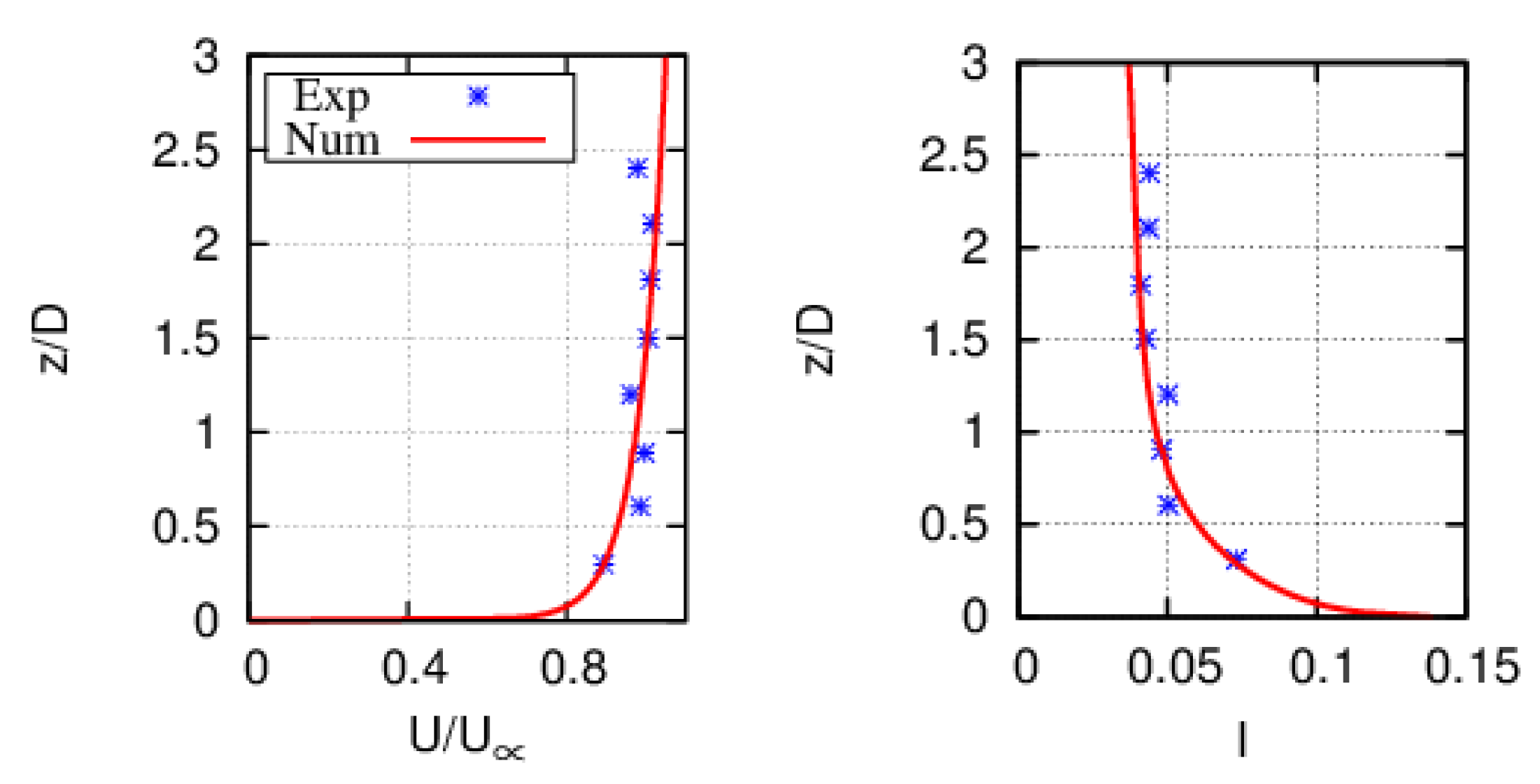
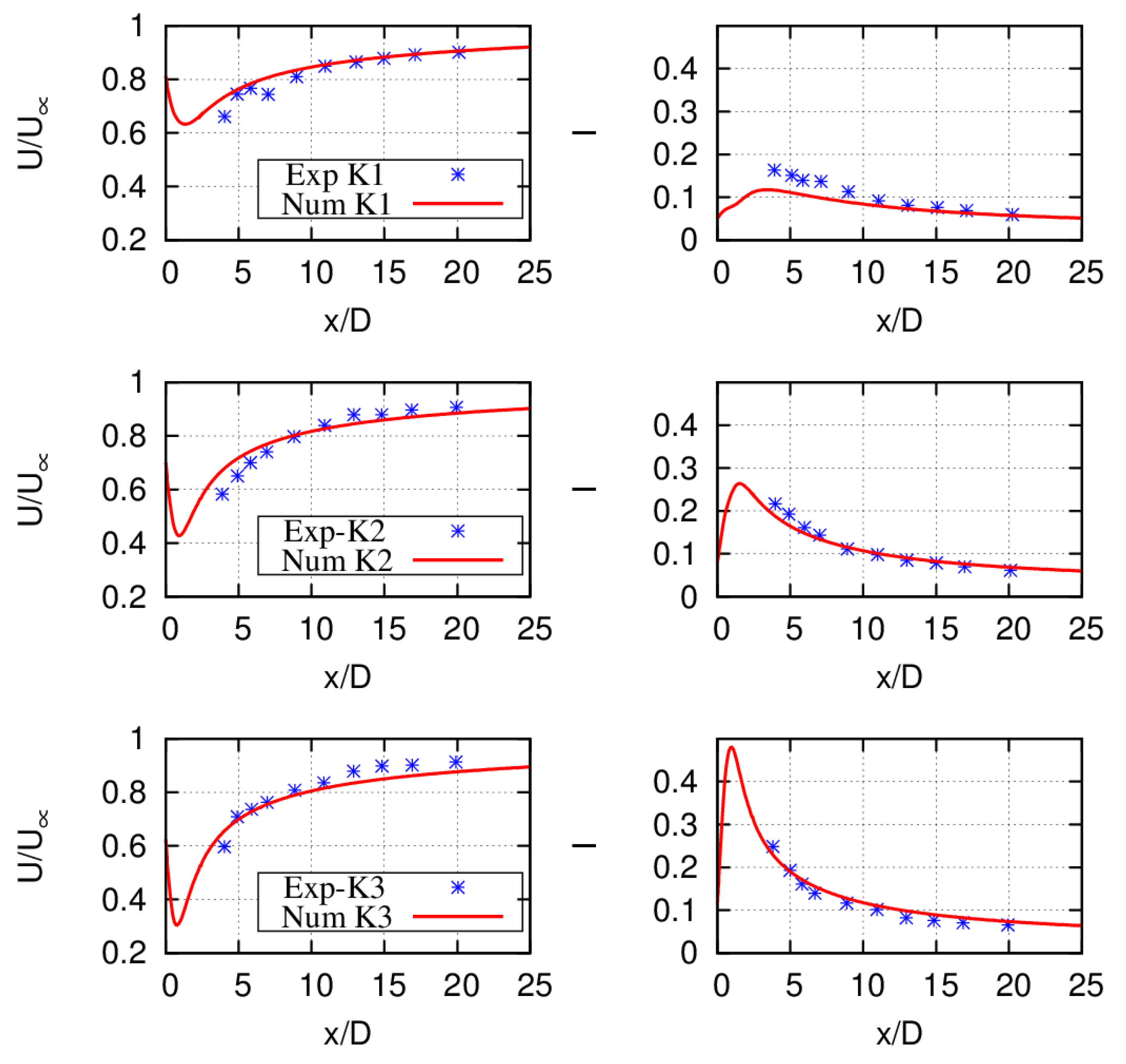
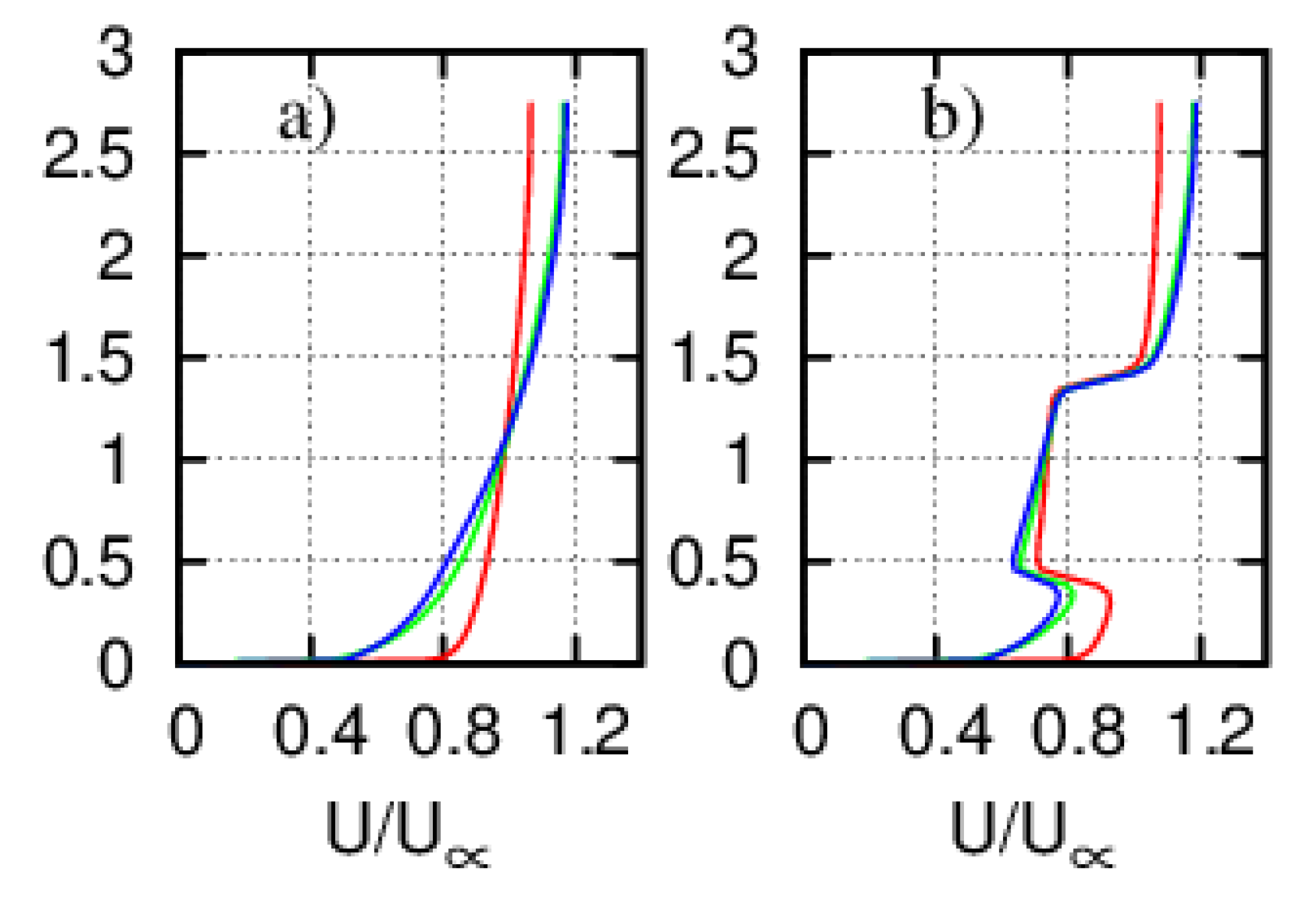
2.2. Model Validation: Flow Past a Porous Disk

The model results are now validated against the experimental measurements of Harrisson et al., 2010 [40] providing measurements of the turbulence intensity and the velocity behind a non-rotating porous disk representing a tidal turbine. The experiments are carried out in a circulating current flume 21 m in length and 1.35 m in width, with a water depth of 0.3 m. The porous disk representing the turbine has a diameter D of 0.1 m and a thickness e of 0.001 m. The disk is placed at mid-depth and 20 D far from the inlet. Measurements are performed using acoustic doppler velocimetry (Myers and Bahaj [35]). Several resistance coefficient K, corresponding to several disk porosity, have been used.

The dimensions of the calculation fluid domain were defined according to the circulating water channel used by Myers and Bahaj [35] and Harrisson et al., 2010 [40] to perform their experiments. The calculation domain is 5 m long and 1.36 m wide. The domain is meshed with 16,867,840 hexahedral elements. The mesh is refined in the disk area where the cell size equals the disk thickness. Symmetry conditions are used on the lateral and top boundaries. The pressure is imposed at the outlet. At the inlet of the domain (Figure 1), the velocity U_I(z) profile and the turbulent kinetic energy k(z) profile are computed with Equations (9)–(12) where U* is the friction velocity, ν is the kinematic viscosity and z₀ is the bed roughness, κ is the eddy dissipation, κ = 0.41 is the Von Karman constant, and I(z) is the turbulence intensity profile (note that, to evaluate the level of turbulence in the wake of the AD, the turbulence intensity I is calculated by using the local maximal velocity to the dimensionless turbulent kinetic energy). I_H is the turbulent intensity at z = H with H the water depth, l = 0.07 H is the vortex characteristic size, and C_μ = 0.09. In Equation (9), considering a smooth bottom, z₀ is assimilated to the thickness of the viscous sublayer and the three parameters velocity U*, z₀, and χ are evaluated by Equation (13) where U_in is the depth-averaged inlet velocity.

$$U_I(z)={{\displaystyle U}}^{*}\left(\frac{1}{\kappa }\ln \left(\frac{z}{z_0}\right)+\chi \right)$$

(9)

$$k(z)=\frac{3}{2}{I}^2(z)U_I{(z)}^2$$

(10)

$$\epsilon =C_{\mu }^{3/4}\frac{k^{3/2}}{l}$$

(11)

$$I(z)=I_H\frac{\ln (H/z_0)}{\ln (z/z_0)}$$

(12)

$$\{\begin{array}{c}{z}_0=11\nu /U^{*}\\ \chi =11\\ U^{*}=\frac{U_{in}}{[z_0/H-1+\ln (H/z_0)]/\kappa +11(z_0-1/H)}\end{array}.$$

(13)

For the model validation, the depth-averaged velocity is set to 0.3 m/s and the ambient turbulent intensity is set to 5% (in accordance with the measurements). Thus, the friction velocity is U* = 7.87 × 10^–3 ms^–1, and z₀ = 2.5 × 10^–8 m is the bed roughness. Special attention was paid to the mesh size in the alignment of the disk. According to Roc et al., in 2013 [32], the results are independent of the mesh size as far the mesh size in the y and z direction are such that ∆y ≤ D/9 and ∆z ≤ D/6. In the present simulations, we opt for a much smaller mesh size, signified by ∆y = D/100 and ∆z = D/100. The residual convergence criteria for velocity and turbulence are 10^–7.

Three different values of C_t are considered (

Table 1. Thrust and power coefficients for three resistance coefficients K studied in this paper. The validation of these results is based on a comparison with experimental results that Harrisson [40] obtained for porous disk, with C_t close to the values usually obtained for the Betz Limit.

The Present Numerical Simulations			Experimental Conditions
K	Ct	Cp	Ct
1	0.64	0.51	0.61
2	00.89	0.59	0.86
3	0.98	0.56	0.94

). For a flow without blockage effects, the Betz limit is reached when C_t = 0.89, which corresponds to a resistance coefficient K of 2. Numerical results obtained with this value of K have been compared to the experimental values [40] measured for C_t =0.86 (Table 1). As noticed in [38], the model predictions fit the measurements either in terms of velocity or turbulence intensity. Simulations with K = 1 and K = 3 also show good velocity predictions (Figure 2). The greatest model discrepancies are located in the near wake. It is probably due to an overproduction of the turbulent kinetic energy in the AD [38], which accelerates the mixing effect in the near wake. This overproduction seems to be more remarkable in the case of low resistance case K = 1. Noteworthy, for the Alderney Race application, is that the longitudinal spacing between two consecutive lines of turbines is 7.5D. At this distance from the disk, the satisfactory agreement between model and experimental data is observed either in terms of flow velocity or turbulence intensity (Figure 2).

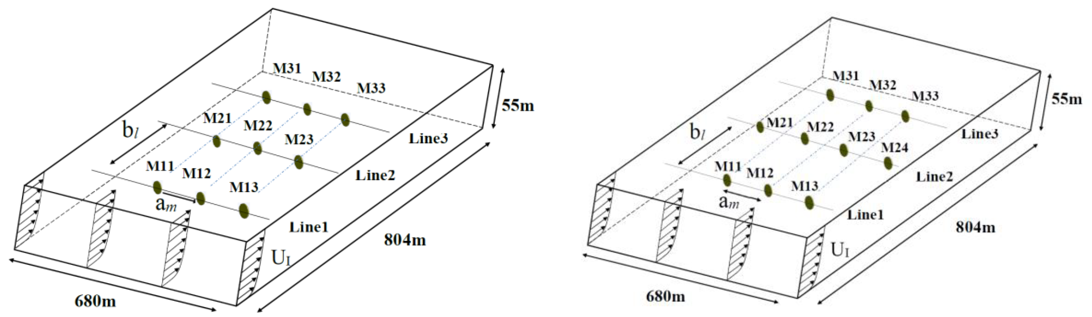
2.3. Model Configuration: Wake-Field Study

The method is now applied to a pilot tidal farm located in the Raz Blanchard. Two layout configurations are considered (Figure 3): Aligned with 9 machines (A) and staggered with 10 machines (S). The calculation domain is 804 m long and 680 m wide. The depth is 55 m. The turbine diameter (D) is 20 m. The turbine thickness (e) is set to 1 m. The turbine axis is located 18 m above the bottom. Myers and Bahaj [1] first suggested a longitudinal spacing of 15 D and a lateral one of 3 D. More recently, Vennell et al. [41] in a review paper indicated that a minimal inter-row spacing of 5 D is recommended. Finally, Bai et al. [20] demonstrate that the appropriate lateral distance, according to the power extraction, is approximately 2.5 D, whereas the minimum inter-row spacing should be 6 D.

For the present purpose, the tidal farm is constituted of three lines of turbines separated by a longitudinal distance b = 7.5 D. The lateral spacing between turbines, from center to center, is set to a = 3 D. Garrett and Cummins [42] theoretically derived the limit of power extraction from the flow by using the so-called linear momentum actuator disk theory (1D-LMADT). Nishino and Willden [43] compared 1D-LMADT to 3D RANS AD computation results obtained for a single machine in a channel and they also applied a similar approach [44,45] to a partial tidal fence. Considering the definition of the local blockage, B_L (the ratio between a single device area and the local passage cross-sectional area) and the global blockage, B_G (the ratio between the total device area and the channel cross-sectional area), proposed in Garrett and Cummins [42] and in Nishino and Willden [44,45], the blockage values are B_L = 0.1 and B_G = 0.03. According to Garret and Cummins [42], a local blockage of 0.1 should give a maximum power coefficient of 0.72 by using the relationship Cp_max=16/27 (1-B_L)^-2 for a single device (which is beyond the limit of Betz, Cp_max =16/27).

The turbine arrangement is symmetric with respect to x- and y-axes. The first line is situated 20 D behind the inlet (left). The domain is covered by a non-uniform Cartesian mesh containing 10,904,400 elements (44,391,533 nodes) with a refinement in the vicinity of the machines. At the bottom, a no-slip condition is used whereas a slip condition is applied at the top. The ratio of disk thickness over mesh size ratio is 2.5 in the x-direction and 1.25 in the y- and the z-directions.

For the present purpose, the wake-field model (Fluent model) is forced with tidal conditions representative of the Raz Blanchard. Those conditions have been extracted (at the selected point) from a regional model named Telemac2D. This model solves the shallow non-linear equations using a finite element formulation [46]. The Telemac2D results (water levels and depth-averaged current velocities) have been validated with the in-situ measurements of [47]. The Telemac2D model indicates that the annual power density, defined as 1/2ρU³ (where U is the depth averaged velocity magnitude), is 5.22 kW/m² at the study site. The period retained for this study corresponds to a mean tide. Results have been extracted between 19:21 on 24 January 2005 and 07:28 on 25 January 2005. The model regional model shows that the local hydrodynamics is influenced by a large eddy that appears north of La Hague Cape, as shown in Figure 4. When the eddy develops (during flood tide), the current velocities vary in direction, which results in a large directional spreading. The current rose representation (Figure 5) highlights a significant tidal asymmetry (in both magnitude and direction) between ebb and flood. The temporal evolution of the flow velocity and the water depth during the study period is represented in Figure 6. Those data have been used to build the vertical profiles of current velocities imposed at the boundaries of the local (fluent) model. To this end, we used Equations (9)–(12) and (14), which apply for rough seabed.

$$\{\begin{array}{c}{z}_0=R/33\\ \chi =0\\ U^{*}=\frac{\kappa U_{in}(H-z_0)}{[z_0-H+H\ln (H/z_0)]}\end{array}$$

(14)

where R is the bed roughness.

During the studied period, the water depth at the extraction point varies between 52.92 and 57.15 m. Sensitivity tests indicate that the water depth has a negligible effect on the total production (<1%). We, therefore, use a unique depth value for all simulations (H = 55 m).

At the extraction point, the optimal direction (the direction maximizing the annual power extraction) was 64° with respect to the north direction. This direction was used to orientate the frame of the wake-field model (and to compute the misalignment with respect to the predominant direction). Then, periods when velocity magnitudes were smaller than 1 m/s were neglected, and the others were discretized temporally. Finally, we obtained 20 tidal conditions representative of the studied mean tide (

Table 2. Boundary conditions calculated with the regional model (Figure 7). The angle is expressed in nautical convention. The incidence is given with respect to the optimal flow direction (the x axis of the local model frame).

Number of the Simulation	Time (h)	Uin (m/s)		Angle (deg)	Incidence (deg)
1	0	2.2	R1	8.9	8.9
2	0.6	1.9		15.1	15.1
3	1.22	1.6		23.2	23.2
4	1.82	0.9		35.9	35.9
5	2.88	0.9	Regime 2 (R2)	161.4	18.6
6	3.43	1.8		162.3	17.7
7	4	2.3		174.0	6.0
8	4.55	2.3		177.6	2.4
9	5.12	2.4		175.8	4.2
10	5.67	2.5		175.2	4.8
11	6.22	2.5		175.1	4.8
12	6.78	2.3		175.3	4.7
13	7.33	2.0		175.6	4.4
14	7.9	1.6		176.0	4.0
15	8.45	0.9		176.2	3.8
16	9.73	0.9	Regime 1 (R1)	358.5	1.5
17	10.37	1.8		0.0	0.0
18	10.98	2.3		2.7	2.7
19	11.62	2.5		6.7	6.9
20	12.25	2.4		12.5	12.5

). In Table 2, the regimes 1 and 2 correspond to the flood and the ebb, respectively. Those 20 tidal conditions were then used to force the wake-field model. We, thus, performed a unique non-stationary simulation with Telemac2D and 20 stationary simulations with the fluent model.

The power of each machine P_ij is calculated with Equation (15) where U_d is the local velocity (along x-axis). The power P_i and the mean power P_im of a given line are given by Equation (16) and the total power of the tidal farm P_farm is calculated with Equation (17). N_i and N_l are, respectively, the number of machines of the line i^th and the total number of lines. During the flood (regime 1), the turbines of lines 2 and 3 are located downstream from line 1, whereas during the ebb (regime 2), the turbines of lines 1 and 2 are located downstream from the turbines of line 3.

$$P_{ij}=F_t{U}_d=\frac{1}{2}K\rho S{U}_d^3$$

(15)

$$P_i={\displaystyle {\sum }_{j=1}^{Nj}{P}_{ij}}$$

(16)

$$P_{farm}={\displaystyle {\sum }_{i=1}^{Ni}{P}_i}$$

(17)

When turbines are placed in array, their wakes interact in different ways [48] and the inflow of a given turbine could be affected by one or several wakes. The most common wake interaction corresponds to a configuration where one turbine is in the wake of another. This interaction is named tandem operation. When two machines placed side by side interact and form a merged wake, the interaction is referred to as interference operation. When the inflow of a turbine is partly affected by one or more wakes, the interaction is named overlapping. To highlight different types of flow interactions occurring within the array, maps of velocity deficit (18) will be plotted.

$$U_{def}=1-\frac{U(x,y,z)}{U_I(z)}$$

(18)

For each layout, two scenarios are examined. The first one corresponds to the velocity and incidence angles introduced in Table 2. It will be referred as the realistic case with incidence angle (RWI). The second scenario consists of “switching off” the incidence angle (the current reverses twice per tide but remains parallel to the x-axis; it varies in magnitude). It is referred to as realistic case without incidence angle (RWOI).

The ratio between the averaged power production per line in the RWI and the RWOI cases is an indicator of the influence of the current incidence on the power. This ratio power indicator is noted RP =P_im(RWI)/P_im(RWOI). A value close to 1 indicates that the flow obliquity has a negligible influence on the production. A value smaller than 1 indicates that the flow obliquity reduces the production and vice versa. The energy produced by the farm during the tidal cycle is also computed as well as the energy per line. Finally, as the number of machines of the two layouts differs (9 devices in the aligned layout and 10 devices in the staggered layout), the mean energy per device has been computed, which permits an unbiased comparison.

Several values of resistance coefficient K and ambient turbulent intensity are used (

Table 3. The different numerical experiments performed in this paper.

I (%)	K	Layout	Scenario	R (m)
5	1	S and A	RWOI and RWI	-
5	2	S and A	RWOI and RWI	-
5	3	S and A	RWOI and RWI	-
10	2	S and A	RWOI and RWI	2
15	2	S and A	RWOI and RWI	5

). The inlet formulation for I_H=5% is related to Equation (13) whereas, for higher turbulence intensities, the relations for rough bed is used (Equation (14)).

3. Results

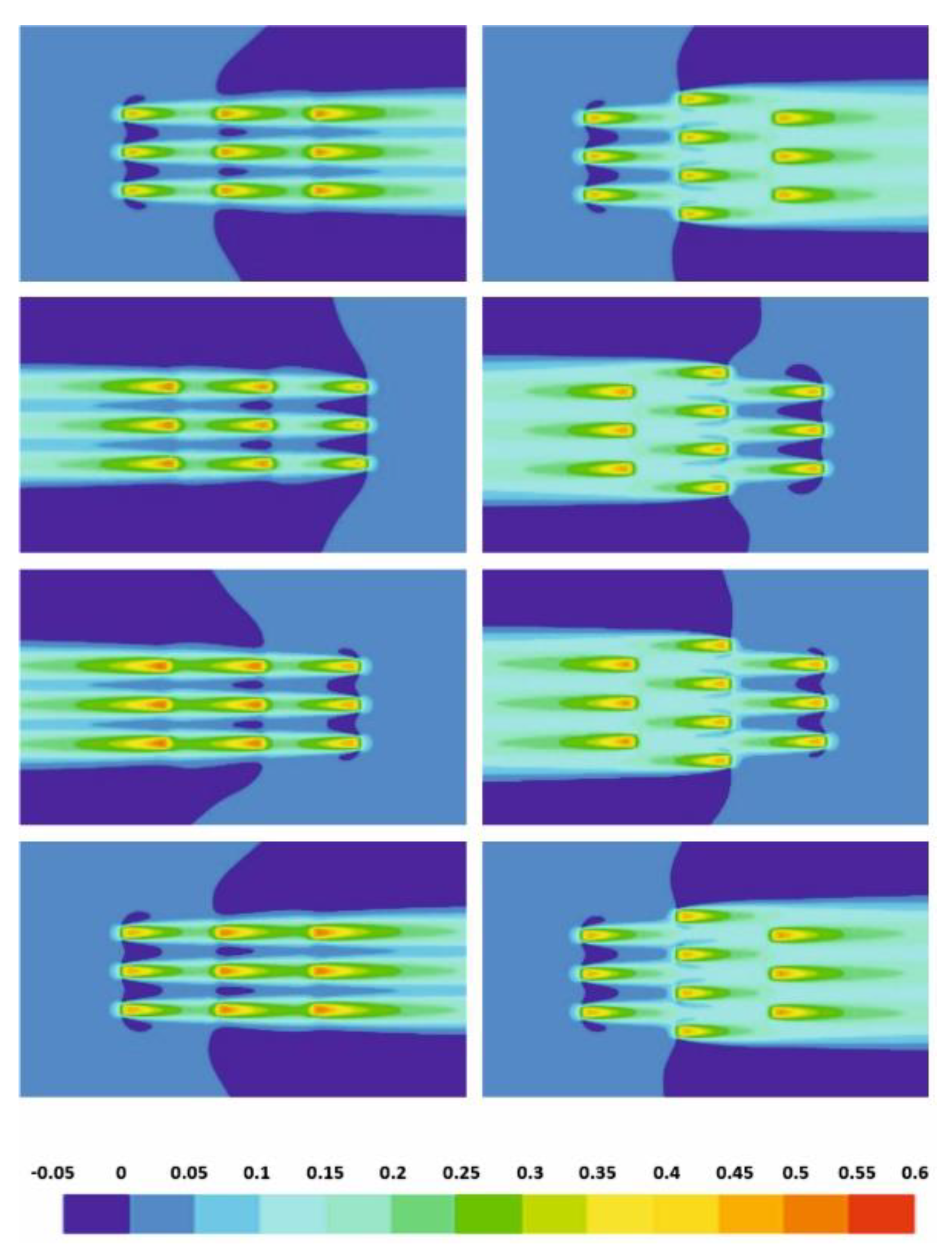
3.1. Effect of Layout

First, the case with K = 2 and I = 5% has been considered. Figure 7 and Figure 8 represent maps of velocity deficit (Equation (18)). The time evolution of the mean power per line (P_im) is represented in Figure 10. For both RWOI and RWI cases, three types of flow interactions (overlapping, interference, and tandem) can be observed (Figure 8 and Figure 9).

For the A-RWOI case (aligned layout without incidence), machines of the three lines (M1j, M2j, M3j) are systematically in tandem situation (Figure 7 left). During the flood, the turbines of the two lines located downstream (lines 2 and 3) produce significantly less than the linear turbines upstream (line 1). During the ebb, the power extracted by the machines of the line 2 is lower than the power extracted by the machines of the line 3 (Figure 9c). This is due to a greater flow recovery between line 2 and line 3 than between lines 1 and 2. This higher flow recovery is imputed to a greater turbulence intensity as the turbulent intensity increases each time the flow passes through a line of turbines.

For the S-RWOI case (staggered layout without incidence), the turbines of lines 1 and 3 are placed in tandem and they are affected by the superposition of the wakes induced by the turbines of line 2 (Figure 7, right). There is a significant difference in production between line 1 and line 3, which depends on the orientation of the current (considering if the line is located upstream or downstream). The turbines of the 2nd line are only slightly affected by the upstream turbines by wake overlapping. The mean power of the line 2 is similar to the one of the upstream line of machines (Figure 9b).

The staggered configuration is supposed to be advantageous compared to the aligned layout [49]. This is confirmed by our results when the flow obliquity is zero: The staggered layout leads to a greater energy production (10.57 MWh /per machine) compared to the aligned layout (8.64 MWh/per machine) (Table 5). This is mainly due to the smaller production of the second line of machines of the aligned arrangement.

In the case of A-RWI case (Figure 8, left) (aligned layout with incidence), the overlapping configuration prevails, and the power extracted by the two downstream lines (Figure 9c) is higher than the one obtained without incidence (Figure 9d). The difference in production between the upstream line and the other lines is more significant during regime 2 than during regime 1.

With St-RWI case (Figure 8 right) (staggered layout with incidence), the wakes overlap, and the power of the second line is significantly reduced in comparison to the aligned layout case (Figure 9a). Occasionally, three machines are placed in tandem, which leads to a noticeable decrease in power (Figure 8, right bottom). By way of illustration, it occurs at t = 12.25 h when the incidence angle is close to 10° or at t = 0 h (Figure 9f) when the incidence angle is 8.9°. In such configurations, although the turbines are placed in a staggered layout, the flow obliquity is such that the turbines M13, M23, and M33 (or M12, M22, M31) are aligned.

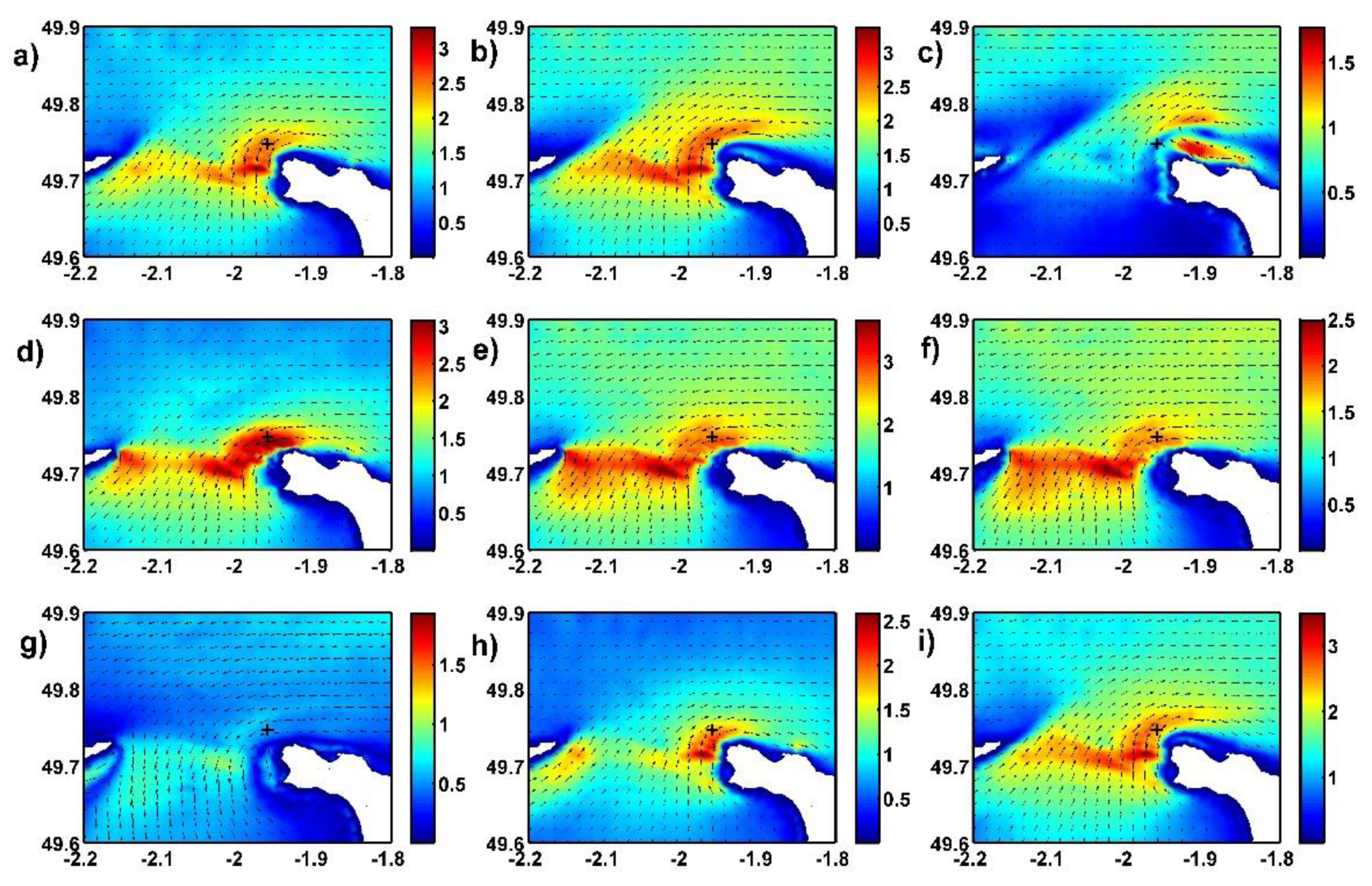
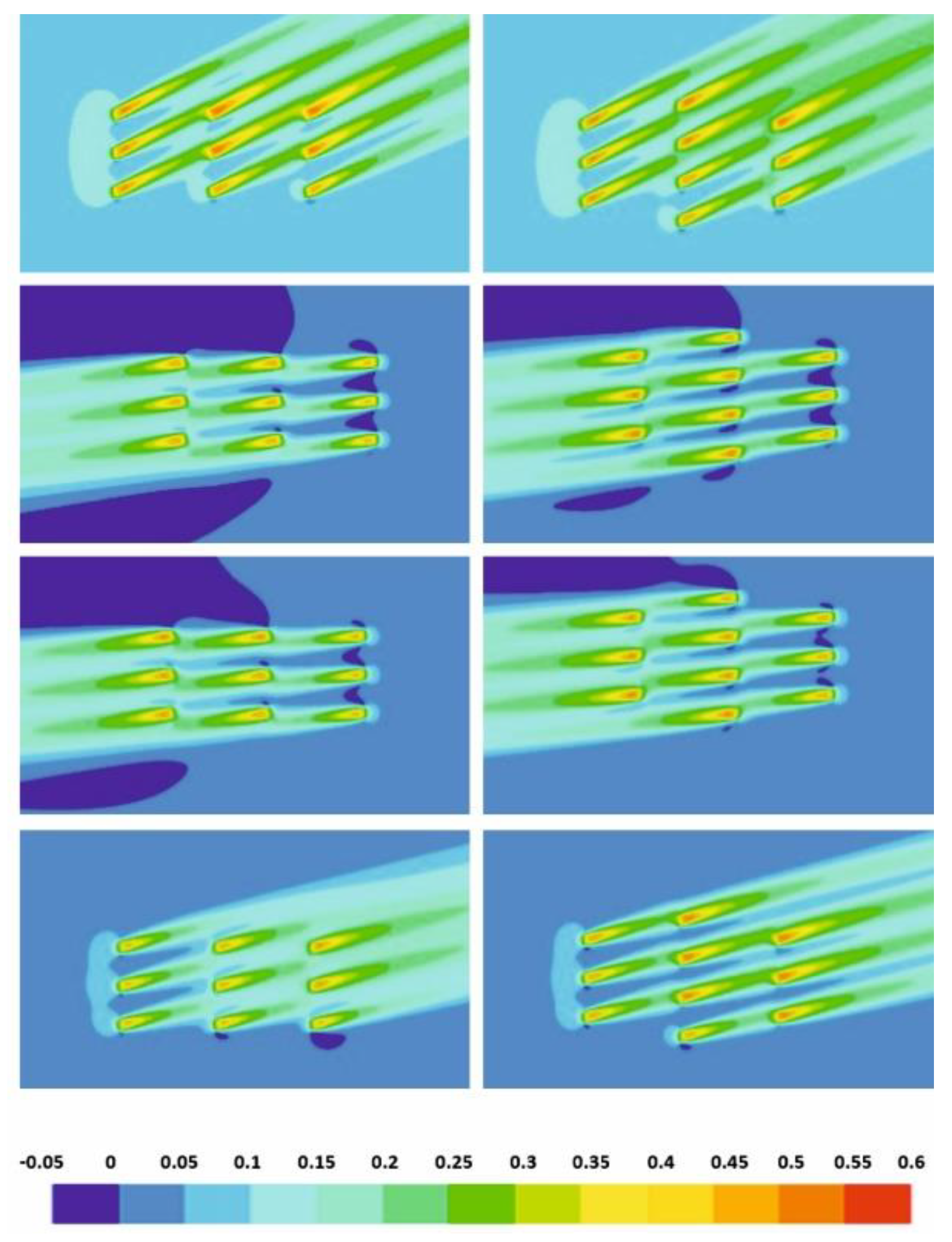
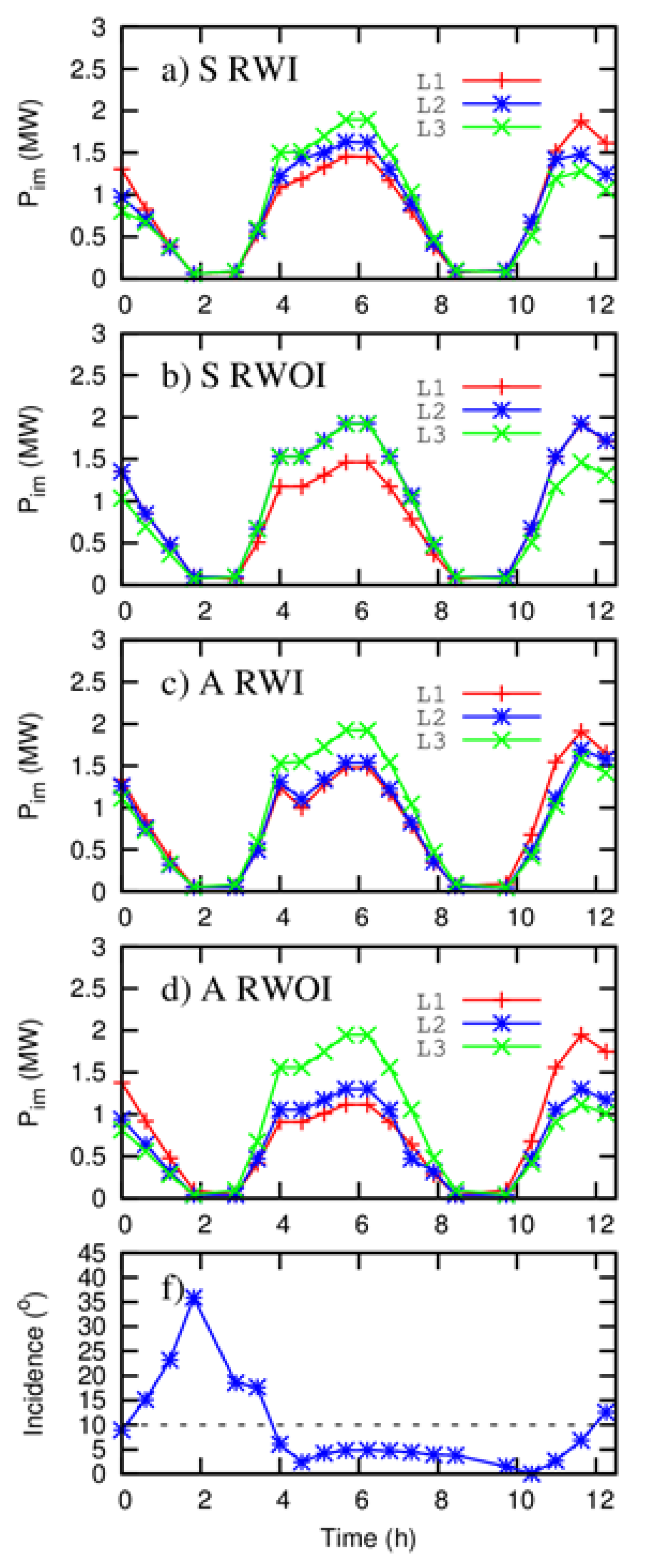
3.2. Effect of Flow Obliquity

The influence of flow obliquity on the production is different when considering a staggered or an aligned layout (Figure 9). Whereas the flow obliquity increases the power of the aligned turbines, it reduces the power of the staggered turbines. It reduces the overall production of the staggered farm as well as the mean production per device (Table 5). The energy reduction is −8.5% (from 105.72 MWh to 96.73 MWh) for the staggered layout and the energy increase is +11.3% for the aligned layout. Finally, when the current varies around the predominant direction (RWI), the gain in using a staggered layout (rather than an aligned layout) is very small (9.62 MWh/per machine for the aligned layout and 9.67 MWh/per machine for the staggered layout) (Table 5). This indicates that the staggered arrangement is not, systematically, the most suitable layout.

The effect of the flow obliquity is complex and differs according to the type of layout, the line of machine, and the regime (Figure 10). As an example, the production of line 1 is only slightly modified by the flow obliquity during regime 1 whereas the power of line 2 significantly decreases during the two regimes. To discriminate the effect of the flow obliquity during ebb and flood tides, the RP indicator is computed per regime for both aligned and the staggered layout (

Table 4. Ratio between P_im(RWI) and P_im(RWOI) for K = 2 and I = 5% configurations. The results are averaged per regime.

K	I%	Layout	Regime	Line 1	Line 2	Line 3
1	5%	A	1	0.88	1.08	1.14
			2	1.24	1.17	0.97
		S	1	0.88	0.79	0.89
			2	1.03	0.89	0.97
2	5%	A	1	0.90	1.17	1.22
			2	1.28	1.22	0.97
		S	1	0.90	0.79	0.91
			2	1.01	0.86	0.97
3	5%	A	1	0.90	1.19	1.23
			2	1.32	1.23	0.97
		S	1	0.90	0.77	0.91
			2	1.01	0.83	0.97
2	10%	A	1	0.88	1.05	1.10
			2	1.17	1.13	0.95
		S	1	0.89	0.79	0.84
			2	0.90	0.84	0.96
2	15%	A	1	0.89	1.02	1.06
			2	1.12	1.10	0.96
		S	1	0.89	0.80	0.83
			2	0.87	0.85	0.96

).

With regards to the line located upstream (line 1 during regime 1 and line 3 during regime 2), the value of RP is smaller than 1 (0.9 for line 1 during R1 and 0.97 for line 3 during R2). This means that the turbines produce less when the flow comes obliquely, which is due to a reduction of the normal velocity component (with respect to the devices’ axis, an analogous calculation of P_ij, where the x-axis component of U_d is replaced by its magnitude, highlights the impact of the flow obliquity on the energy production of the aligned layout (K=2 – I=5%) (cf. Table 4). Indeed, for the RWOI case, we observe a change of 2.3% between to the two different energy calculations. Note that this gap increases until 7.8% for the RWI case. With respect to the 2nd line, the ratio RP shows opposite trends depending on the layout. For the staggered layout, the flow obliquity has a negative effect on the second line production (the ratio is 0.79 or 0.86) whereas the aligned layout creates a positive effect (the ratio is 1.17 or 1.22). For the aligned layout, the energy production is lower than the one of line 1 or 3 (

Table 5. Energy produced during the mean tide (MWh) for K = 1, 2, and 3 and t = 5% configurations. The energy is calculated either for each line or for all the turbines (farm). The column farm/N, where N is the number of machines of the farm, indicates the mean energy delivered per turbine. Energies are computed for the two scenarios (RWOI and RWI) and aligned and staggered layout. (*) The power captured by a machine is calculated by using the local velocity along x-axis (15). Replacing the local velocity along x by the local velocity magnitude puts to the fore the impact of the flow obliquity on the production of a tidal farm.

K	I%	Layout	Scenario	Line 1	Line 2	Line 3	Farm	Farm/N
1	5%	A	RWOI	19.11	16.87	21.13	57.12	6.35
			RWI	21.20	20.17	22.34	63.71	7.08
		S	RWOI	22.86	33.34	22.88	78.07	7.81
			RWI	21.82	28.98	22.09	72.89	7.29
2	5%	A	RWOI	25.82	22.88	29.03	77.73	8.64
			RWI	28.54	27.21	30.80	86.54	9.62
		S	RWOI	29.16	45.65	30.92	105.72	10.57
			RWI	28.57	38.38	29.78	96.73	9.67
		A (*)	RWOI	26.43	23.38	29.74	79.54	8.84
			RWI	30.81	29.42	33.06	93.30	10.37
3	5%	A	RWOI	26.78	22.11	30.83	79.72	8.86
			RWI	30.50	28.29	33.11	91.90	10.21
		S	RWOI	31.44	50.84	33.75	116.03	11.60
			RWI	30.74	41.28	32.47	104.49	10.45
2	10%	A	RWOI	24.48	22.02	27.40	73.90	8.21
			RWI	26.33	25.53	28.32	80.19	8.91
		S	RWOI	28.4	42.91	29.82	101.12	10.11
			RWI	25.99	35.54	27.75	89.28	8.93
2	15%	A	RWOI	23.74	21.66	26.37	71.78	7.98
			RWI	25.16	24.58	27.06	76.80	8.53
		S	RWOI	27.34	40.57	28.60	96.51	9.65
			RWI	24.58	33.95	26.56	85.27	8.53

A) regardless of whether the incidence is switched off or not.

Indeed, the turbines of line 2 are, most of the time, in overlapping or tandem configuration. When the current is parallel to the turbines’ axis, the turbines of line 2 are in tandem, which is the worst configuration. When the flow arrives obliquely, the turbines of line 2 move from a tandem to an overlapping configuration (Figure 8, left) and, thus, produce slightly more (Figure 9c,d). Concerning the S-RWI case, there could be a variety of wake interactions along line 2. The turbines can be located either in an unperturbed flow (the turbine located on the side (M21 or M24)) or in a funneled flow (turbines M22 and M23 benefit from the flow acceleration between the turbines of the line of turbines located upstream). They can also be in an overlapping or a tandem configuration. In the overlapping configuration (Figure 7, right), the power of line 2 is significantly reduced in comparison to the aligned layout case (Figure 9a). Over the tide, the energy produced is equivalent to the one of the other lines 28.57/3 ≈ 38.38/4 ≈ 29.78/3. For the S-RWOI case, turbines are always placed in the free steam. Thus, line 2 produces more than the two other lines thanks to the funnel effect (45.65/4 > 29.16/3 and 45.65/4 > 30.92/3).

For the RWOI case, the machines placed downstream (line 3 during R1 and line 1 during R2) are in tandem configuration (aligned layout) or wake overlapping (staggered layout). Depending on the layout, the distance between two consecutive machines is b for the aligned layout and 2b for the staggered one. When the spacing between turbines is 2b, the flow recovery is nearly complete, and the turbines located downstream thus produces as much as the turbines located in the free stream. When the incidence is “switched off”, the flow interaction between the wakes moves from overlapping/interference to tandem/overlapping. The flow obliquity favors the production of the aligned layout (1.22 for L3 and R1; 1.28 for L1 and R2) and reduces the production of the staggered layout (0.86 for L3 and R1; 0.97 for L1 and R2). Occasionally, three machines are placed in tandem, which leads to a significant decrease in power (Figure 8, right bottom). For instance, it occurs at t = 12.25 h when the incidence angle is close to 10° or at t = 0 h (Figure 9f) when the incidence angle is 8.9°. In such configurations, though the turbines are placed in a staggered layout, the flow obliquities in such that the turbines M13, M23, and M32 (or M12, M22, M31) are aligned.

3.3. Effect of Resistance Coefficient and Ambient Turbulence Level

The analysis has been extended to examine several values of the resistance coefficient and ambient turbulence level (Table 4 and Table 5).

When K increases from 2 to 3, the total energy (Table 5) increase is about 40% and 48% for the A-RWOI and the S-RWOI cases, respectively. This increase is around 44% with the RWI configurations. The findings concerning the effect of the incidence obtained for the baseline case (I = 5% K = 2) are also applied to the configurations (I = 5% K = 1) and (I = 5% K = 3) (the obliquity increases the power produced by the aligned layout and reduces the power produced by the staggered layout; the mean energy produced by each machine is the same with both the aligned and the staggered layout when the current is multi-directional). However, it should be noted that the baseline trend is exacerbated with a greater value of the coefficient of resistance. The relative reduction of the energy between RWOI and RWI for the “staggered layout’ increases from 8.5% when K = 2 to 9.9% when K = 3. For the aligned layout, the energy increase remains close to +11.3% for K = 1 and K = 2 and reaches +15.2% for K = 3.

The impact of the ambient turbulence intensity on the farm production is estimated by comparing simulations with different turbulence intensity values I = 5%, 10%, and 15%; here, a constant K receives the value of 2 (Table 3). It is observed that the energy produced (Table 5) decreases with turbulence intensity when it gets higher values whether the obliquity is “switched off” or not. This reduction is imputed to the modification of the vertical profile of x-velocity when the turbulent intensity increases (Figure 11). The differences between cases RWI and RWOI are coherent with the previously described configurations. For the staggered configuration, the relative reduction of the energy between RWOI and the RWI cases is −13.2 for I = 10 and 15%. For the aligned layout, the gain in energy is +11.3 for I = 5% and +6.9% for I = 15%.

Similarl to the baseline case, the ratio RP is greater than 1 for the downstream lines of the aligned layout and lower than 1 for the downstream lines of the staggered layout. Nevertheless, the amplitude of the ratio for the aligned arrangement decreases with increasing values of I (Table 4). For example, considering line 2 of the aligned layout during the ebb (R2), RP varies from 1.17 in the case I = 5% to 1.02 with I = 15%. The same tendency is perceived for the downstream lines (L1 in regime R2 and L3 in regime R1). Considering the staggered arrangement, the ambient turbulence intensity does not significantly modify the ratio RP of the line 2. However, it significantly affects the downstream line of turbines (L1 in R2 and L3 in R1). For instance, the RP of line L1 in regime R2 varies from 1.01 for I = 5% to 0.87 for I = 15%). Noteworthily, the RP of the lines of turbines located in the free stream (L1 in R1 and L3 in R2) is unchanged when the turbulence intensity varies from I = 5% to 15%.

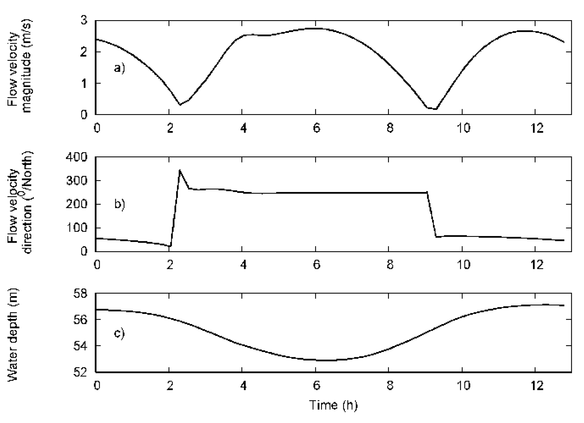
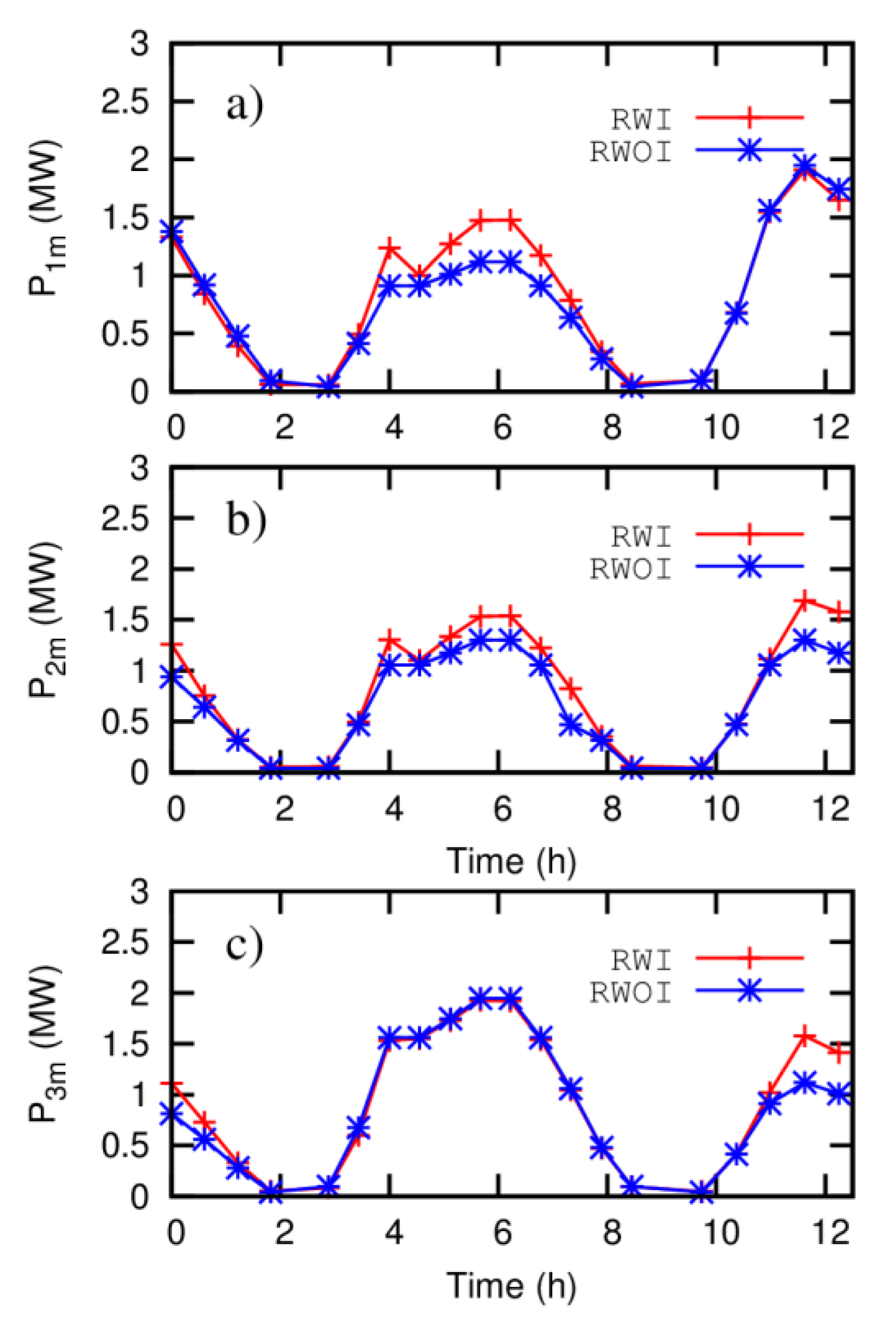
3.4. Effect of the Tidal Asymmetry

Similar to other tidal straits [7,8,10,17], the flow in the Raz Blanchard is characterized by an asymmetry of the tidal current amplitude as well as a directional spreading around a predominant direction. Depending on the current direction (ebb or flood), the turbines of lines 1 and 3 are alternately in the free stream or located downstream the array. The asymmetry of the current amplitude is 6%, which leads to a systematic difference between the averaged powers captured by L1 and L3. Moreover, the available kinetic energy fluctuates during the ebb and the flood. Our results highlight that, for both layouts, the current misalignment causes a reduction in the averaged power of about 10% for L1 (in the free stream during t during the flood tide). This decrease falls to 3% for L3 during the ebb. What is the cause of this disparity? At the studied site, the angles of incidence (with respect to the predominant direction) are relatively small (7° on average during the studied period) during the ebb. However, during the flood, the presence of a large-scale eddy located northward of the Hague Cape deviates the current, which leads to mean and maximum angles of incidence of 12° and 35° (during the studied period). Indeed, as the flow obliquity, with respect to turbines’ axis, increases, the axial projected area of the turbine decreases, and the kinetic energy extracted drops as well. These results are in accord with Galloway [50] and Frost’s [10] considerations for a horizontal axial turbine. As a matter of fact, Frost [10] noticed a reduction of C_p of 7% for an incidence angle of the incoming flow of 10° and a value greater than 22% for an incidence angle of 20°.

As earlier stated, the direction used to orientate the frame of the wake-field model maximizes the extraction of the hydrodynamic power. This orientation is determined from a one-year-long simulation and is, therefore, representative of a mean value. For the present study, we focus on particular tidal conditions (mean tide). Under those conditions, the mean current direction is not perfectly aligned with the yearly averaged predominant direction.

4. Conclusions

The influence of a time-varying current direction on the energy production of a pilot tidal farm has been analyzed using a quasi-steady RANS approach where the tidal turbines are represented as actuator disks. The interactions between wakes induced by adjacent turbines have been simulated considering two arrangements: Staggered (10 turbines) and aligned (9 turbines). The tidal farm model is forced using boundary conditions (velocity direction and magnitude) recommended by a regional model of the Alderney Race (France). Effects of the incidence between the incoming flow and the turbines’ axis, the resistance coefficients, and the turbulence intensities are considered. The principal findings are listed below:

• The flow obliquity influences, in a different way, the production of the staggered and the aligned arrays. Whereas it increases the production of the aligned layout, it reduces the production of the staggered layout. Mean energy produced per machine is almost the same for both layouts.
• There is a significant difference between the production during the ebb and the flood tides.
• Increasing turbulent intensity reduces the positive effect of the flow obliquity on the aligned layout production and restricts the negative effect on the staggered layout production.
• The increase of ambient turbulence seems to slightly reduce the energy production of both layouts.

Additional simulations are therefore required to generalize the results and to improve understanding the influence of turbulence intensity influences on the energy production of a tidal farm. Our future works will consider the blockage effect, which is believed to have a strong influence on the flow dynamics in a pilot farm. Those simulations are realized with a quasi-steady model, that does not account for the rapid variation of direction and flow speed inerrant to turbulent area. Such a problem must be resolved with a finer model as presented by Bourgoin et al. [51] but the computation time is a limit to its use. The waves have an effect on the flow speed and the direction as noted by Lewis et al. [52]. Their effects on the energy production should be study further.

References

1. Myers, L.E.; Bahaj, A.S. Simulated electrical power potential harnessed by marine current turbine arrays in the Alderney Race. Renew. Energy 2005, 30, 1713–1731. [Google Scholar] [CrossRef]
2. Lo Brutto, O.A.; Barakat, M.; Guillou, S.S.; Thiébot, J.; Gualous, H. Influence of the wake effect on electrical dynamics of commercial tidal farms: Application to the Alderney Race (France), Methodology for estimating the French tidal current energy resource. IEEE Trans. Sustain. Energy 2018, 9, 321–332. [Google Scholar] [CrossRef]
3. Segura, E.; Morales, R.; Somolinos, J.A. Cost Assessment Methodology and Economic Viability of Tidal Energy Projects. Energies 2017, 10, 1086. [Google Scholar] [CrossRef]
4. Nguyen, V.T.; Guillou, S.S.; Santa Cruz, A.; Thiébot, J. Numerical simulation of a pilot tidal farm using actuator disks, influence of a time-varying current direction. In Proceedings of the Grand Renewable Energy Conference, Tokyo, Japan, 27 July–1 August 2014. [Google Scholar]
5. Bahaj, A.S.; Myers, L.E. Analytical estimates of the energy yield potential from the Alderney Race (Channel Islands) using marine current energy converters. Renew. Energy 2004, 29, 1931–1945. [Google Scholar] [CrossRef]
6. Thiébot, J.; du Bois, P.B.; Guillou, S. Numerical modeling of the effect of tidal stream turbines on the hydrodynamics and the sediment transport—Application to the Alderney Race (Raz Blanchard), France. Renew. Energy 2015, 75, 356–365. [Google Scholar] [CrossRef]
7. Guillou, N.; Chapalain, G. Tidal turbine’s layout in a stream with asymmetry and misalignment. Energies 2017, 10, 1892. [Google Scholar] [CrossRef]
8. Guillou, N.; Chapalain, G. Assessing the impact of tidal stream energy extraction on the Lagragian circulation. Appl. Energy 2017, 203, 321–332. [Google Scholar] [CrossRef]
9. Neill, S.P.; Hashemi, R.M.; Lewis, M.J. The role of tidal asymmetry in characterizing the tidal energy resource of Orkney. Renew. Energy 2014, 68, 337–350. [Google Scholar] [CrossRef]
10. Frost, C.; Evans, P.S.; Harrolds, M.J.; Mason-Jones, A.; O’Doherty, D.M.; O’Doherty, T. The impact of axial flow misalignment on a tidal turbine. Renew. Energy 2017, 113, 1333–1344. [Google Scholar] [CrossRef]
11. Guillou, N.; Neill, S.P.; Robins, P.E. Characterising the tidal stream power resource around France using a high-resolution harmonic database. Renew. Energy 2018, 123, 706–718. [Google Scholar] [CrossRef] [Green Version]
12. Coles, D.S.; Blunden, L.S.; Bahaj, A.S. Assessment of the energy extraction potential at tidal sites around the Channel Islands. Energy 2017, 124, 171–186. [Google Scholar] [CrossRef]
13. Campbell, R.; Martinez, A.; Letetrel, C.; Rio, A. Methodology for estimating the French tidal current energy resource. Int. J. Mar. Energy 2017, 19, 256–271. [Google Scholar] [CrossRef]
14. Thiébaut, M.; Sentchev, A. Asymmetry of tidal currents off the W. Brittany coast and assessment of tidal energy resource around the Ushant Island. Renew. Energy 2017, 105, 735–747. [Google Scholar] [CrossRef]
15. Lewis, M.; Neill, S.P.; Robins, P.E.; Hashemi, M.R. Resource assessment for future generations of tidal-stream energy arrays. Energy 2015, 83, 403–415. [Google Scholar] [CrossRef] [Green Version]
16. Modali, P.K.; Kolekar, N.; Banerjee, A. Performance and wake characteristics of a tidal turbine under yaw. IMEJ 2018, 1, 41–50. [Google Scholar]
17. Tian, W.; VanZwieten, J.H.; Pyakurel, P.; Li, Y. Influences of yaw angle and turbulence intensity. Energy 2016, 111, 104–116. [Google Scholar] [CrossRef]
18. Gebreslassie, M.G.; Belmont, M.R.; Taylor, G.R. Comparison of Analytical and CFD Modelling of the Wake Interactions of Tidal Turbines. In Proceedings of the 10th EWTEC Conference, Aalborg, Denmark, 2–5 September 2013. [Google Scholar]
19. Divett, T.; Vennell, R.; Stevens, C. Optimization of multiple turbine arrays in a channel with tidally reversing flow by numerical modelling with adaptive mesh. Philos. Trans. R. Soc. A 2013, 371, 20120251. [Google Scholar] [CrossRef] [PubMed]
20. Bai, G.; Li, J.; Fan, P.; Li, G. Numerical investigations of the effects of different arrays on power extractions of horizontal axis tidal current turbines. Renew. Energy 2013, 53, 180–186. [Google Scholar] [CrossRef]
21. Olczak, A.; Stallard, T.; Feng, T.; Stansby, P.K. Comparison of a RANS blade element model for tidal turbine arrays with laboratory scale measurements of wake velocity and rotor thrust. J. Fluids Struct. 2016, 64, 87–106. [Google Scholar] [CrossRef]
22. Mycek, P.; Gaurier, B.; Germain, G.; Pinon, G.; Rivoalen, E. Experimental study of the turbulence intensity effects on marine current turbines behaviour. Part II: Two interacting turbines. Renew. Energy 2014, 68, 876–892. [Google Scholar] [CrossRef] [Green Version]
23. Malki, R.; Masters, I.; Williams, A.J.; Croft, T.N. Planning tidal stream turbine array layouts using a coupled blade element momentum—Computational fluid dynamics model. Renew. Energy 2014, 63, 46–54. [Google Scholar] [CrossRef]
24. Draper, S.; Nishino, T. Centered and staggered arrangements of tidal turbines. J. Fluid Mech. 2014, 739, 72–93. [Google Scholar] [CrossRef]
25. Gebreslassie, M.G.; Taylor, G.R.; Belmont, M.R. Investigation of the performance of a staggered configuration of tidal turbines using CFD. Renew. Energy 2015, 80, 690–698. [Google Scholar] [CrossRef] [Green Version]
26. Churchfield, M.J.; Li, Y.; Moriarty, P.J. A large-eddy simulation study of wake propagation and power production in an array of tidal-current turbines. Philos. Trans. R. Soc. A 2013, 371, 20120421. [Google Scholar] [CrossRef] [PubMed] [Green Version]
27. Myers, L.E.; Bahaj, A.S. An experimental investigation simulating flow effects in first generation marine current energy converter arrays. Renew. Energy 2012, 37, 28–36. [Google Scholar] [CrossRef] [Green Version]
28. Belhache, M.; Guillou, S.; Grangeret, P.; Mouaze, D.; Santa Cruz, A. Wake numerical study of a vertical marine current turbine. Houille Blanche 2014, 6, 73–77. [Google Scholar] [CrossRef]
29. Wu, B.; Zhang, X.; Chen, J.; Xu, M.; Li, S.; Li, G. Design of high-efficient and universally applicable blades of tidal stream turbine. Energy 2013, 60, 187–194. [Google Scholar] [CrossRef]
30. Frost, C.; Morris, C.E.; Mason-Jones, A.; O’Doherty, D.M.; O’Doherty, T. The effect of tidal flow directionality on tidal turbine performance characteristics. Renew. Energy 2015, 78, 609–620. [Google Scholar] [CrossRef] [Green Version]
31. Antheaume, S.; Maître, T.; Achard, J.L. Hydraulic Darrieus turbines efficiency for free fluid flow conditions versus power farms conditions. Renew. Energy 2008, 33, 2186–2198. [Google Scholar] [CrossRef]
32. Roc, T.; Conley, D.C.; Greaves, D. Methodology for tidal turbine representation in ocean circulation model. Renew. Energy 2013, 51, 448–464. [Google Scholar] [CrossRef] [Green Version]
33. Lee, S.H.; Lee, S.H.; Jang, K.; Lee, J.; Hur, N. A numerical study for the optimal arrangement of ocean current turbine generators in the ocean current power parks. Curr. Appl. Phys. 2010, 10, S137–S141. [Google Scholar] [CrossRef]
34. Hunter, W.; Nishino, T.; Willden, R.H. Investigation of Tidal Turbine Array Tuning Using 3D Reynolds-Averaged Navier-Stokes Simulations. Int. J. Mar. Energy 2015, 10, 39–51. [Google Scholar] [CrossRef]
35. Myers, L.E.; Bahaj, A.S. Experiment analysis of the flow field around horizontal axis tidal turbines by use of scale mesh disk rotor simulators. Ocean Eng. 2010, 37, 218–227. [Google Scholar] [CrossRef]
36. Castellani, F.; Vignaroli, F. An application of the actuator disc model for wind turbine wakes calculations. Appl. Energy 2013, 101, 432–440. [Google Scholar] [CrossRef]
37. Taylor, G.I. The Scientific Papers of Sir Geoffrey Ingram Taylor; Batchelor, G.K., Ed.; Cambridge University Press: Cambridge, UK, 1963. [Google Scholar]
38. Nguyen, V.T.; Guillou, S.S.; Thiébot, J.; Santa Cruz, A. Modelling turbulence with an Actuator Disk representing a tidal turbine. Renew. Energy 2016, 97, 625–635. [Google Scholar] [CrossRef]
39. Lewis, M.; Neill, S.P.; Robins, P.E.; Hashemi, M.R.; Waer, S. Characteristics of the velocity profile at tidal-stream energy sites. Renew. Energy 2017, 114, 258–272. [Google Scholar] [CrossRef]
40. Harrison, M.E.; Batten, W.M.J.; Myers, L.E.; Bahaj, A.S. Comparison between CFD simulation and experiments for predicting the far wake of horizontal axis tidal turbines. IET Renew. Power Gener. 2010, 4, 613–627. [Google Scholar] [CrossRef]
41. Vennell, R.; Funke, S.W.; Draper, S.; Stevens, C.; Divett, T. Designing large arrays of tidal turbines: A synthesis and review. Renew. Sustain. Energy Rev. 2015, 41, 454–472. [Google Scholar] [CrossRef]
42. Garrett, C.; Cummins, P. The efficiency of a turbine in a tidal channel. J. Fluid Mech. 2007, 588, 243–251. [Google Scholar] [CrossRef] [Green Version]
43. Nishino, T.; Willden, R.H.J. Effect of 3-D channel blockage and turbulent wake mixing on the limit of power extraction by tidal turbines. Int. J. Heat Fluid Flow 2012, 37, 123–135. [Google Scholar] [CrossRef]
44. Nishino, T.; Willden, R.H.J. The efficiency of an array of tidal turbines partially blocking a wide channel. J. Fluid Mech. 2012, 708, 596–606. [Google Scholar] [CrossRef]
45. Nishino, T.; Willden, R.H.J. Two-scale dynamics of flow past a partial cross-stream array of tidal turbines. J. Fluid Mech. 2013, 730, 220–244. [Google Scholar] [CrossRef] [Green Version]
46. Hervouet, J.M. Hydrodynamics of Free Surface Flows: Modelling with the Finite-Element Method; John Wiley & Sons Ltd.: West Sussex, UK, 2007; p. 340. [Google Scholar]
47. du Bois, P.B.; Dumas, F.; Solier, L.; Voiseux, C. In-Situ database toolbox for short-term dispersion model validation in macro-tidal seas, application for 2D-model. Cont. Shelf Res. 2012, 36, 63–82. [Google Scholar] [CrossRef]
48. Palm, M.; Huijsmans, R.; Pourquie, M. The Applicability of Semi-Empirical Wake Models for Tidal Farms. In Proceedings of the 9th European Wave and Tidal Energy Conference, Southampton, UK, 5–9 September 2011. [Google Scholar]
49. Bai, L.; Spence, R.R.G.; Dudzak, G. Investigation of the Influence of Array Arrangement and Spacing on Tidal Energy Converter (TEC) performance using a 3-Dimensional CFD Model. In Proceedings of the 8th European Wave and Tidal Energy Conference, Uppsala, Sweden, 7–10 September 2009; pp. 654–660. [Google Scholar]
50. Galloway, P.; Myers, L.E.; Bahaj, A.S. Experimental and numerical results of rotor power and thrust of a tidal turbine operating at yaw and in waves. In Proceedings of the World Renewable Energy Congress, Linkoping, Sweden, 8–13 May 2011. [Google Scholar]
51. Bourgoin, A.; Guillou, S.S.; Ata, R.; Thiébot, J.; Benhamadouche, S.T. Currents characterization with Large Eddy Simulation. In Proceedings of the 3th Asian Waves and Tides Energy Conference, Taipei, Taiwan, 9–12 September 2018. [Google Scholar]
52. Lewis, M.J.; Neill, S.P.; Hashemi, M.R.; Reza, M. Realistic wave conditions and their influence on quantifying the tidal stream energy resource. Appl. Energy 2014, 136, 495–508. [Google Scholar] [CrossRef] [Green Version]
Figure 1. Vertical profiles of axial velocity (left) and turbulent intensity at the inlet (right). Comparison between numerical results (Num) and experimental (Exp) of Harrisson et al., 2010 [40]. Reproduced with permission from [38], Nguyen et al., Renewable Energy; published by Elsevier, 2016.
Energies 12 02478 g001
Figure 2. Axial normalized velocity (left) and turbulence intensity (right) along the turbine’s axis (x = 0 is the AD position). Comparison between experimental (Exp) (Harrisson et al., 2010) [40] and numerical results (Num) for the 3 values of K tested (cf. Table 1). Note that, to evaluate the turbulence intensity (IT) in the wake of the AD, Equation (10) was applied by using the local maximal velocity to dimensionless the turbulent kinetic energy.
Energies 12 02478 g002
Figure 3. Calculation domains with the localization of the turbines: Aligned layout (left), staggered layout (right). bl = 7.5 D and am = 3 D.
Energies 12 02478 g003
Figure 4. Currents in the Raz Blanchard during a mean tidal cycle. The cross represents the study site. (a) High tide; (b) High tide plus 1/8th of the tidal period; (c) High tide plus 1/4th of the tidal period; (d) High tide plus 3/8th of the tidal period; (e) Low tide; (f) High tide plus 5/8th of the tidal period; (g) High tide plus 3/4th of the tidal period; (h) High tide plus 7/8th of the tidal period; (i) High tide.
Energies 12 02478 g004
Figure 5. Temporal evolution of the representation of (Ux, Uy) extracted at a location point with coordinates (1°57.66’W; 49°44.83’N) during the tidal cycle (tidal rose). Dots correspond to the 20 time-varying flow conditions given in Table 2. The water depth at the extraction point varies between 52.92 and 57.15 m.
Energies 12 02478 g005
Figure 6. Temporal evolution of the flow velocity magnitude (a), flow velocity direction (b), and water depth (c) over a mean tide. The flow directions are expressed following the nautical convention.
Energies 12 02478 g006
Figure 7. Isocontour of velocity deficit in the case without incidence (RWOI) in a tidal farm with an aligned (left) and a staggered layout (right) for time 1.22 h (R1), 4 h, 6.22 h (R2), and 12.25 h (R1).
Energies 12 02478 g007
Figure 8. Isocontour of velocity deficit in the case with incidence (RWI) in a tidal farm with an aligned (left) and a staggered layout (right) for time 1.22 h (R1), 4 h, 6.22 h (R2), and 12.25 h (R1).
Energies 12 02478 g008
Figure 9. Time evolution of the power: (a) Mean power per line Pim (MW) in the case with incidence angle and staggered layout (St RWI); (b) mean power per line Pim (MW) in the case without incidence angle and staggered layout (St RWOI); (c) mean power per line Pim (MW) in the case with incidence angle and aligned layout (Al RWI); (d) mean power per line Pim (MW) in the case without incidence angle and aligned layout (St RWOI); (e) incidence angle.
Energies 12 02478 g009
Figure 10. Time evolution of the mean power per line with and without current incidence: (a) P1 m (MW) for an aligned layout (S); (b) P2 m (MW) for an aligned layout (S); (c) P3 m (MW) for an aligned layout (S).
Energies 12 02478 g010
Figure 11. Dimensionless x-velocity along the domain depth for the inlet velocity v = 2.2 m/s at x = 160 m (a) and at the position of the first row of machines (b); red (5%), green (10%), blue (15%).
Energies 12 02478 g011