Measuring the Time-Frequency Dynamics of Return and Volatility Connectedness in Global Crude Oil Markets


Abstract
1. Introduction
2. Empirical Techniques
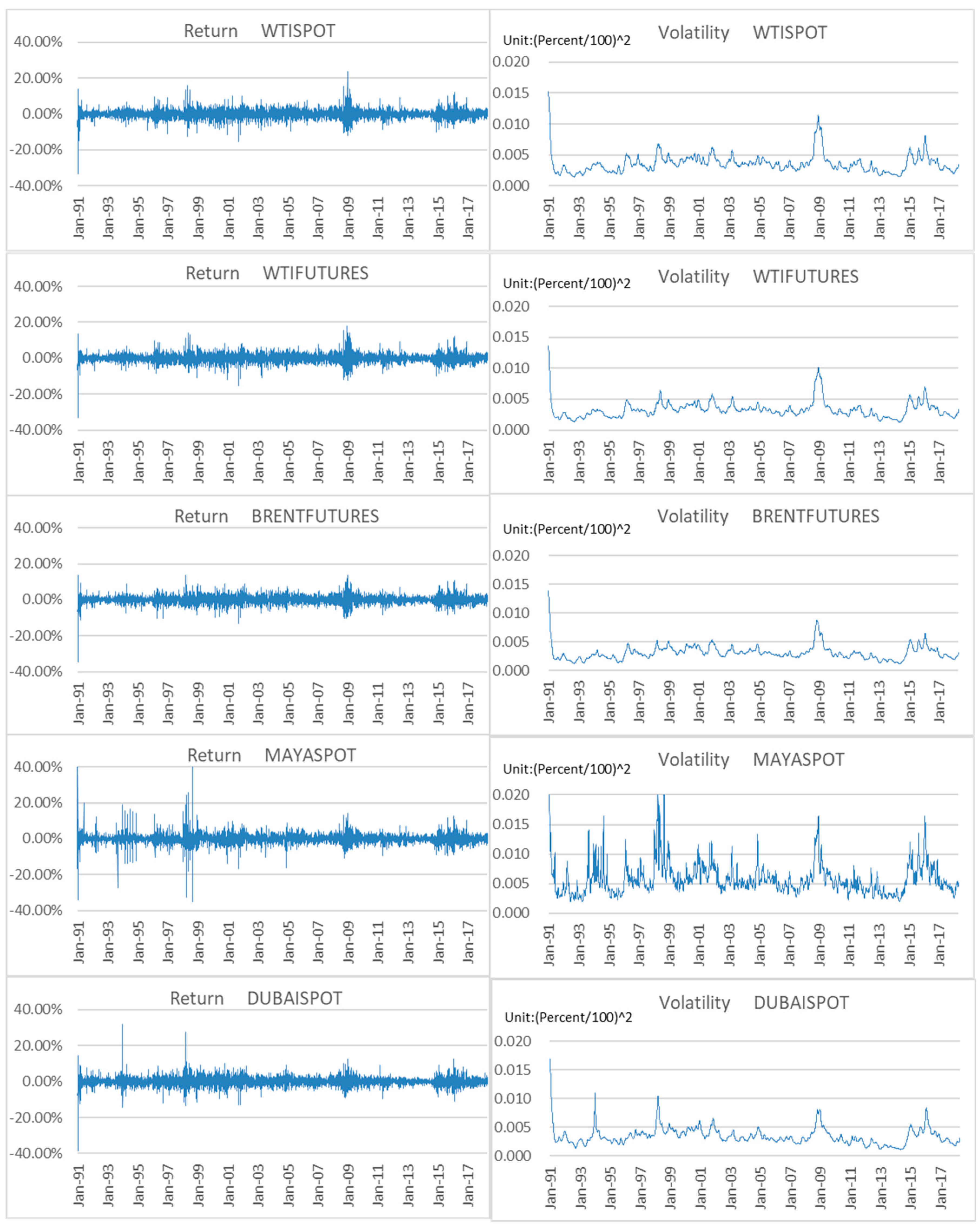
3. Data and Preliminary Analysis
- WTISPOT: West Texas Intermediate (WTI) crude oil spot price
- WTIFUTURES: WTI crude oil futures price
- BRENTFUTURES: Brent crude oil futures price
- MAYASPOT: Maya crude oil spot price
- DUBAISPOT: Dubai crude oil spot price
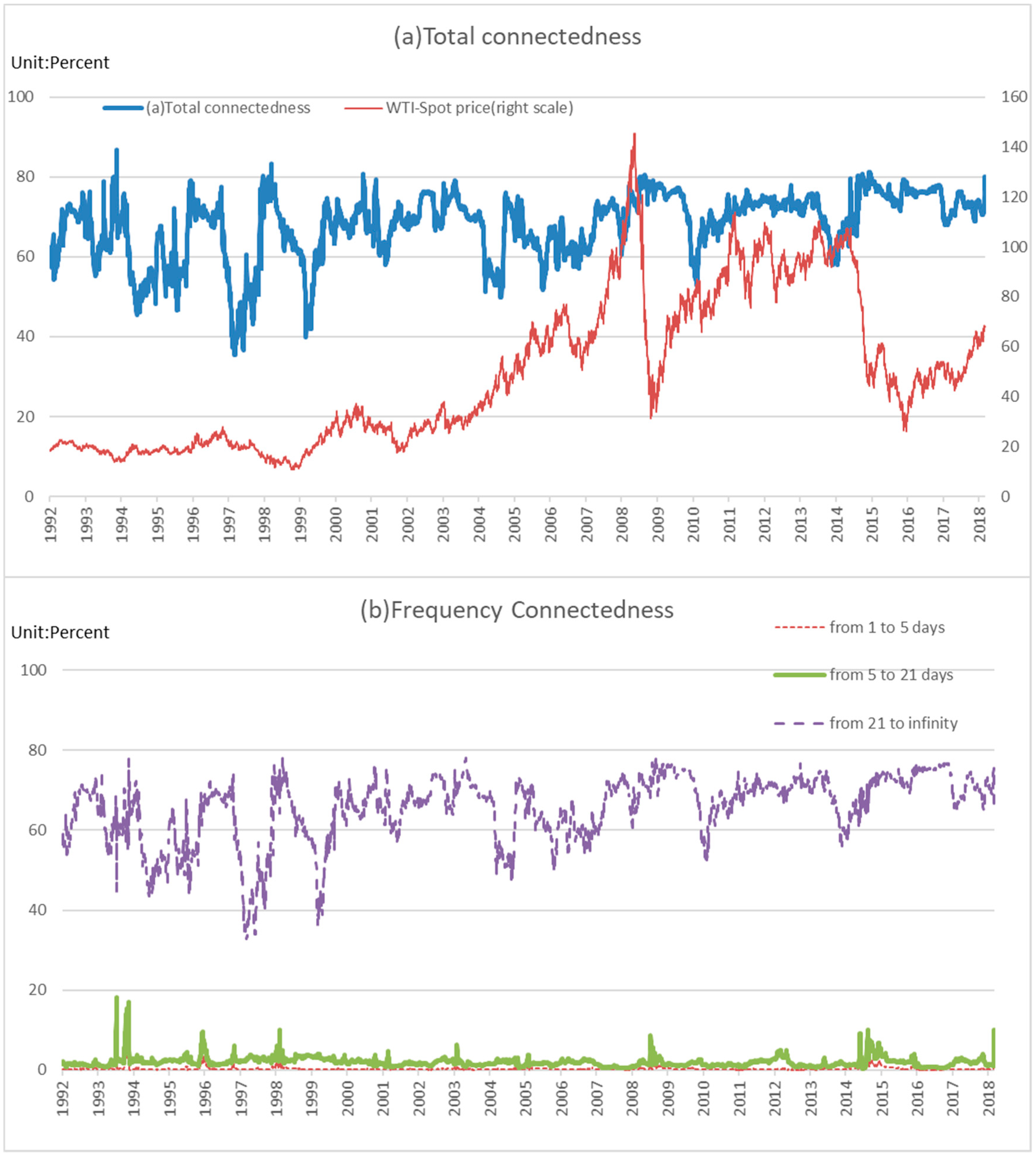
4. Estimation Results
4.1. Spillover Results
4.2. Moving-Window Analysis
5. Concluding Remarks
Author Contributions
Funding
Acknowledgments
Conflicts of Interest
References
- Ross, S.A. Information and volatility: No-arbitrage martingale approach to timing and resolution irrelevancy. J. Financ. 1989, 44, 1–17. [Google Scholar] [CrossRef]
- Fleming, J.; Kirby, C.; Ostdiek, B. Information and volatility linkages in the stock, bond, and money markets. J. Financ. Econ. 1998, 49, 111–137. [Google Scholar] [CrossRef]
- Diebold, F.X.; Yilmaz, K. Better to give than receive: Predictive directional measurement of volatility spillovers. Int. J. Forecast. 2012, 28, 57–66. [Google Scholar] [CrossRef]
- Barunik, J.; Koenda, E.; Vácha, L. Asymmetric connectedness of stocks: Bad and good volatility spillovers. J. Financ. Mark. 2016, 27, 55–78. [Google Scholar] [CrossRef]
- Bae, K.H.; Karolyi, A.; Stulz, R. A new approach to measuring financial contagion. Rev. Financ. Stud. 2003, 16, 717–763. [Google Scholar] [CrossRef]
- Dungey, M.; Martin, V.L. Unravelling financial market linkages during crises. J. Appl. Econom. 2007, 22, 89–199. [Google Scholar] [CrossRef]
- Morana, C.; Beltratti, A. Comovements in international stock markets. J. Int. Financ. Mark Inst. Money 2008, 18, 31–45. [Google Scholar] [CrossRef]
- Ehrmann, M.; Fratzscher, M.; Rigobon, R. Stocks, bonds, money markets and exchange rates: Measuring international financial transmission. J. Appl. Econom. 2011, 26, 948–974. [Google Scholar] [CrossRef]
- Beirne, J.; Gieck, J. Interdepencence and contagion in global asset markets. Rev. Int. Econ. 2014, 22, 639–659. [Google Scholar] [CrossRef]
- Bae, K.H.; Zhang, X. The cost of stock market integration in emerging markets. Asia Pac. J. Financ. Stud. 2015, 44, 1–23. [Google Scholar] [CrossRef]
- Lehkonen, H. Stock market integration and the global financial crisis. Rev. Financ. 2015, 19, 2039–2094. [Google Scholar] [CrossRef]
- Aït-Sahalia, Y.; Hurd, T. Portfolio choice in markets with contagion. J. Financ. Econom. 2016, 14, 1–28. [Google Scholar] [CrossRef]
- Ang, A.; Bekaert, G. International asset allocation with regime shifts. Rev. Financ. Stud. 2002, 15, 1137–1187. [Google Scholar] [CrossRef]
- Balcilar, M.; Demirer, R.; Hammoudeh, S.; Nguyen, D.K. Risk spillovers across the energy and carbon markets and hedging strategies for carbon risk. Energy Econ. 2016, 54, 159–172. [Google Scholar] [CrossRef]
- Scholes, M.S. Crisis and risk management. Am. Econ. Rev. 2000, 90, 17–21. [Google Scholar] [CrossRef]
- Chang, C.P.; Lee, C.C. Do oil spot and futures move together? Energy Econ. 2015, 50, 379–390. [Google Scholar] [CrossRef]
- Kaufmann, R.K.; Ullman, B. Oil prices, speculation, and fundamentals: Interpreting causal relations among spot and futures prices. Energy Econ. 2009, 31, 550–558. [Google Scholar] [CrossRef]
- Pan, Z.; Wang, Y.; Yan, L. Hedging crude oil using refined product: A regime switching asymmetric DCC approach. Energy Econ. 2014, 46, 472–484. [Google Scholar] [CrossRef]
- Chang, C.L.; McAleer, M.; Tansuchat, R. Crude oil hedging strategies using dynamic multivariate GARCH. Energy Econ. 2011, 33, 912–923. [Google Scholar] [CrossRef]
- Toyoshima, Y.; Nakajima, T.; Hamori, S. Crude oil hedging strategy: New evidence from the data of the financial crisis. Appl. Financ. Econ. 2013, 23, 1033–1041. [Google Scholar] [CrossRef]
- Nicolau, M.; Palomba, G. Dynamic relationships between spot and futures prices: The case of energy and gold commodities. Resour. Policy 2015, 45, 130–143. [Google Scholar] [CrossRef]
- Chen, P.F.; Lee, C.C.; Zeng, J.H. The relationships between spot and futures oil prices: Do structural breaks matter? Energy Econ. 2014, 43, 206–217. [Google Scholar] [CrossRef]
- Wang, Y.; Wu, C. Are crude oil spot and futures prices cointegrated? Not always! Econ. Model. 2013, 33, 641–650. [Google Scholar] [CrossRef]
- Maslyuk, S.; Smyth, R. Cointegration between oil spot and future prices of the same and different grades in the presence of structural change. Energy Policy 2009, 37, 1687–1693. [Google Scholar] [CrossRef]
- Huang, B.N.; Yang, C.W.; Hwang, M.J. The dynamics of a nonlinear relationship between crude oil spot and futures prices: A multivariate threshold regression approach. Energy Econ. 2009, 31, 91–98. [Google Scholar] [CrossRef]
- Bekiros, S.D.; Diks, C.G.H. The relationship between crude oil spot and futures prices: Cointegration, linear, and nonlinear causality. Energy Econ. 2008, 30, 2673–2685. [Google Scholar] [CrossRef]
- Bhar, R.; Hamori, S. Causality in variance and the type of traders in crude oil futures. Energy Econ. 2005, 27, 527–539. [Google Scholar] [CrossRef]
- Lee, C.C.; Zeng, J.H. The impact of oil price shocks on stock market activities: Asymmetric effect with quantile regression. Math. Comput. Simul. 2011, 81, 1910–1920. [Google Scholar] [CrossRef]
- Balcilar, M.; Bekiros, S.; Gupta, R. The role of news-based uncertainty indices in predicting oil markets: A hybrid nonparametric quantile causality method. Empir. Econ. 2017, 53, 879–889. [Google Scholar] [CrossRef]
- Yun, W.C.; Kim, H.J. Hedging strategy for crude oil trading and the factors influencing hedging effectiveness. Energy Policy 2010, 38, 2404–2408. [Google Scholar] [CrossRef]
- Diebold, F.X.; Yilmaz, K. Financial and Macroeconomic Connectedness: A Network Approach to Measurement and Monitoring, 1st ed.; Oxford University Press: Oxford, UK, 2014. [Google Scholar]
- Diebold, F.X.; Yilmaz, K. Measuring financial asset return and volatility spillovers, with application to global equity markets. Econ. J. 2009, 119, 158–171. [Google Scholar] [CrossRef]
- Barunik, J.; Krehlik, T. Measuring the frequency dynamics of financial connectedness and systemic risk. J. Financ. Econom. 2018, 16, 271–296. [Google Scholar] [CrossRef]
- Koop, G.; Pesaran, M.H.; Potter, S.M. Impulse Response Analysis in Nonlinear Multivariate Models. J. Econom. 1996, 74, 119–147. [Google Scholar] [CrossRef]
- Pesaran, H.H.; Shin, Y. Generalized Impulse Response Analysis in Linear Multivariate Models. Econ. Lett. 1998, 58, 17–29. [Google Scholar] [CrossRef]
- Kastner, G.; Frühwirth-Schnatter, S. Ancillarity-sufficiency interweaving strategy (ASIS) for boosting MCMC estimation of stochastic volatility models. Comput. Stat. Data Anal. 2014, 76, 408–423. [Google Scholar] [CrossRef]
- Yang, L.; Hamori, S. Modeling the dynamics of international agricultural commodity prices: A comparison of GARCH and stochastic volatility models. Ann. Financ. Econ. 2018, 13, 1850010. [Google Scholar] [CrossRef]
- Jarque, C.M.; Bera, A.K. Test for normality of observations and regression residuals. Int. Stat. Rev. 1987, 55, 163–172. [Google Scholar] [CrossRef]
- Phillips, P.C.B.; Perron, P. Testing for a unit root in time series regression. Biometrika 1988, 75, 335–346. [Google Scholar] [CrossRef]
- Said, S.E.; Dickey, D.A. Testing for unit roots in autoregressive-moving average models of unknown order. Biometrika 1984, 71, 599–607. [Google Scholar] [CrossRef]
- Schwarz, G. Estimating the dimension of a model. Ann. Stat. 1978, 6, 461–464. [Google Scholar] [CrossRef]
- Tiwari, A.K.; Cunado, J.; Gupta, R.; Wohar, M.E. Volatility spillovers across global asset classes: Evidence from time and frequency domains. Q. Rev. Econ. Financ. 2018. [Google Scholar] [CrossRef]
- Kilian, L. Not all oil price shocks are alike: Disentangling demand and supply shocks in the crude oil market. Am. Econ. Rev. 2009, 99, 1053–1069. [Google Scholar] [CrossRef]
- Chen, W.; Kinkyo, T.; Hamori, S. Macroeconomic Impacts of Oil Prices and Underlying Financial Shocks. J. Int. Financ. Mark. Inst. Money 2014, 29, 1–12. [Google Scholar] [CrossRef]


| No. | Authors | Journal Name | Empirical Technique | Market/Data | Principal Results |
|---|---|---|---|---|---|
| 16 | Chang and Lee (2015) | Energy Economics | Wavelet coherency analysis in time–frequency domain | WTI spot and futures | Long-run cointegration relationship between oil spot and futures prices is found. In addition, the short-run causality is more significant in shorter maturity pairs. |
| 17 | Kaufmann and Ullman (2009) | Energy Economics | Unrestricted vector error correction model (VECM) | WTI spot and futures Brent spot and futures Maya spot Dubai-Fateh spot Bonny light spot | Innovations of spillover first appear in spot prices for Dubai–Fateh and spread to other spot and futures prices while other innovations first appear in the far month contract for West Texas Intermediate and spread to other exchanges and contracts. |
| 18 | Pan et al. (2014) | Energy Economics | Regime switching asymmetric dynamic conditional correlation (DCC) model | WTI spot and futures gasoline and heating oil | To hedge portfolio, regime switching asymmetric DCC model is better model than some conventional multivariate generalized autoregressive conditional heteroscedasticity model (multivariate GARCH model). |
| 19 | Chang et al. (2011) | Energy Economics | Multivariate GARCH | WTI spot and futures | To calculate optimal portfolio weights and optimal hedge ratios, diagonal Baba-Engle-Kraft-Kroner (diagonal BEKK) model is the best model. |
| 20 | Toyoshima et al. (2013) | Applied Financial Economics | Asymmetric DCC Multivariate GARCH | WTI spot and futures | To reduce the variance of hedged portfolio, the performance of models is good in order of Asymmetric DCC, DCC, and Diagonal BEKK. |
| 21 | Nicolau (2015) | Resources Policy | Recursive bivariate VAR model | WTI spot and futures | Cointegration relationship between oil spot and futures prices is found, and weak exogeneity exists. |
| 22 | Chen et al. (2014) | Energy Economics | Cointegration tests with structural breaks | WTI spot and futures | Authors find one structural break (July 2004) existed in the long-run relationship between spot and futures oil prices. |
| 23 | Wang and Wu (2013) | Economic Modelling | Nonlinear threshold VECM | WTI spot and futures | Cointegration relationship between crude oil spot and futures are found only when the price differentials are larger than the threshold value |
| 24 | Maslyuk and Smyth (2009) | Energy Policy | Residual-based tests for cointegration in models with regime shifts | WTI and Brent spot and futures | Spot and future prices of the same grade as well as spot and futures prices of different grades are cointegrated. |
| 25 | Huang et al. (2009) | Energy Economics | Three-regime VECM | WTI spot and futures | When the spot price is higher than futures price, and the basis is less than certain threshold value, there exists at least one causal relationship between the change of spot price and futures price. |
| 26 | Bekiros and Diks (2008) | Energy Economics | Linear Granger test nonlinear causality test | WTI spot and futures | While the linear causal relationships have disappeared after the cointegration filtering, nonlinear causal linkages in some cases were revealed. |
| 27 | Bhar and Hamori (2005) | Energy Economics | Cross-correlation function approach | Crude oil futures price Crude oil trading volume | One-way causal effect from price to volume in the investigation of crude oil futures market is found. |
| 28 | Lee and Zeng (2011) | Mathematics and Computers in Simulation | Multiple structural breaks test Quantile regression | Average global crude oil price Real stock returns in G7 countries Interest rate Industrial production | The responses of stock markets to oil price shocks are diverse among G7 countries.In many cases, quantile regression estimates are quite different from simple ordinary least squares (OLS) models. |
| 29 | Balcilar et al. (2017) | Empirical Economics | Nonparametric quantile causality test | WTI spot Economic policy uncertainty (EPU) index Equity market uncertainty (EMU) index | For oil returns, EPU and EMU have strong predictive power over the entire distribution barring regions around the median, but for volatility, the predictability virtually covers the entire distribution, with some exceptions in the tails. |
| 30 | Yun et al. (2010) | Energy Policy | Simple OLS | Dubai spot and WTI futures Exchange rate | Authors find that the hedging effectiveness would be improved by considering the intercorrelation between commodity price and exchange rate. |
| a. Descriptive Statistics and Preliminary Tests for Return. | |||||
| Return WTISPOT | Return WTIFUTURES | Return BRENTFUTURES | Return MAYASPOT | Return DUBAISPOT | |
| Observations | 7128 | 7128 | 7128 | 7128 | 7128 |
| Descriptive statistics | |||||
| Mean | 0.040% | 0.038% | 0.036% | 0.054% | 0.042% |
| Median | 0.000% | 0.000% | 0.000% | 0.000% | 0.000% |
| Maximum | 23.709% | 17.833% | 13.767% | 50.330% | 31.757% |
| Minimum | –33.519% | –33.000% | –34.768% | –34.942% | –38.697% |
| Std. Dev. | 2.341% | 2.282% | 2.125% | 2.651% | 2.328% |
| Skewness | –0.180 | –0.227 | –0.518 | 1.195 | –0.032 |
| Kurtosis | 14.487 | 13.688 | 16.458 | 56.240 | 24.376 |
| Normality tests | |||||
| Jarque-Bera | 39,227.840 | 33,991.800 | 54,109.080 | 843,541.300 | 135,714.100 |
| Probability | 0.000 | 0.000 | 0.000 | 0.000 | 0.000 |
| Unit root tests | |||||
| ADF test statistics | –85.810 | –86.409 | –87.795 | –90.269 | –64.635 |
| p-value | 0.000 | 0.000 | 0.000 | 0.000 | 0.000 |
| PP test statistics | –86.438 | –86.858 | –87.832 | –90.132 | –91.714 |
| p-value | 0.000 | 0.000 | 0.000 | 0.000 | 0.000 |
| b. Descriptive Statistics and Preliminary Tests for Volatility. | |||||
| Volatility WTISPOT | Volatility WTIFUTURES | Volatility BRENTFUTURES | Volatility MAYASPOT | Volatility DUBAISPOT | |
| Observations | 7128 | 7128 | 7128 | 7128 | 7128 |
| Descriptive statistics | |||||
| Mean | 0.004 | 0.003 | 0.003 | 0.006 | 0.003 |
| Median | 0.003 | 0.003 | 0.003 | 0.005 | 0.003 |
| Maximum | 0.015 | 0.014 | 0.014 | 0.039 | 0.017 |
| Minimum | 0.001 | 0.001 | 0.001 | 0.002 | 0.001 |
| Std. Dev. | 0.001 | 0.001 | 0.001 | 0.003 | 0.001 |
| Skewness | 2.388 | 2.292 | 2.190 | 3.003 | 2.235 |
| Kurtosis | 12.943 | 12.123 | 13.197 | 21.213 | 13.435 |
| Normality tests | |||||
| Jarque-Bera | 36,139.550 | 30,960.240 | 36,577.650 | 109,230.200 | 38,273.380 |
| Probability | 0.000 | 0.000 | 0.000 | 0.000 | 0.000 |
| Unit root tests | |||||
| ADF test statistics | –7.915 | –6.811 | –8.466 | –11.440 | –8.407 |
| p-value | 0.000 | 0.000 | 0.000 | 0.000 | 0.000 |
| PP test statistics | –8.405 | –8.376 | –9.106 | –12.356 | –9.117 |
| p-value | 0.000 | 0.000 | 0.000 | 0.000 | 0.000 |
| Diebold and Yilmaz (2012) Spillover Table | |||||||
| Return WTISPOT | Return WTIFUTURES | Return BRENTFUTURES | Return MAYASPOT | Return DUBAISPOT | From | ||
| Return WTISPOT | 92.25 | 6.86 | 0.37 | 0.13 | 0.39 | 1.55 | |
| Return WTIFUTURES | 2.96 | 94.89 | 1.35 | 0.12 | 0.67 | 1.02 | |
| Return BRENTFUTURES | 3.14 | 2.71 | 93.59 | 0.28 | 0.29 | 1.28 | |
| Return MAYASPOT | 2.26 | 2.55 | 2.19 | 92.81 | 0.20 | 1.44 | |
| Return DUBAISPOT | 2.74 | 1.99 | 16.42 | 0.60 | 78.25 | 4.35 | |
| To | 2.22 | 2.82 | 4.07 | 0.23 | 0.31 | 9.64 | |
| Barunik and Krehlik (2018) Spillover results | |||||||
| Freq S: The Spillover Table for Band: 3.14 to 0.63. Roughly Corresponds to 1 Days to 5 Days. | |||||||
| Return WTISPOT | Return WTIFUTURES | Return BRENTFUTURES | Return MAYASPOT | Return DUBAISPOT | From_abs | From_wtn | |
| Return WTISPOT | 83.78 | 5.26 | 0.32 | 0.13 | 0.29 | 1.2 | 1.33 |
| Return WTIFUTURES | 2.66 | 85.39 | 0.78 | 0.12 | 0.57 | 0.82 | 0.92 |
| Return BRENTFUTURES | 2.84 | 2.66 | 80.79 | 0.23 | 0.28 | 1.20 | 1.33 |
| Return MAYASPOT | 2.21 | 2.30 | 1.51 | 84.21 | 0.17 | 1.24 | 1.37 |
| Return DUBAISPOT | 2.38 | 1.97 | 13.75 | 0.47 | 75.16 | 3.71 | 4.12 |
| To_abs | 2.02 | 2.44 | 3.27 | 0.19 | 0.26 | 8.17 | |
| To_wtn | 2.24 | 2.71 | 3.63 | 0.21 | 0.29 | 9.08 | |
| Freq M: The Spillover Table for Band: 0.63 to 0.15. Roughly Corresponds to 5 Days to 21 Days. | |||||||
| Return WTISPOT | Return WTIFUTURES | Return BRENTFUTURES | Return MAYASPOT | Return DUBAISPOT | From_abs | From_wtn | |
| Return WTISPOT | 6.78 | 1.26 | 0.03 | 0.00 | 0.08 | 0.27 | 3.57 |
| Return WTIFUTURES | 0.25 | 7.33 | 0.43 | 0.00 | 0.09 | 0.15 | 1.99 |
| Return BRENTFUTURES | 0.25 | 0.05 | 9.72 | 0.04 | 0.01 | 0.07 | 0.88 |
| Return MAYASPOT | 0.04 | 0.19 | 0.49 | 6.40 | 0.02 | 0.15 | 1.94 |
| Return DUBAISPOT | 0.29 | 0.03 | 2.04 | 0.09 | 2.49 | 0.49 | 6.37 |
| To_abs | 0.16 | 0.30 | 0.60 | 0.03 | 0.04 | 1.13 | |
| To_wtn | 2.15 | 3.97 | 7.77 | 0.36 | 0.51 | 14.76 | |
| Freq L: The Spillover Table for Band: 0.15 to 0.01. Roughly Corresponds to More than 21 Days. | |||||||
| Return WTISPOT | Return WTIFUTURES | Return BRENTFUTURES | Return MAYASPOT | Return DUBAISPOT | From_abs | From_wtn | |
| Return WTISPOT | 1.70 | 0.34 | 0.02 | 0.00 | 0.02 | 0.08 | 3.29 |
| Return WTIFUTURES | 0.06 | 2.17 | 0.14 | 0.00 | 0.02 | 0.05 | 1.92 |
| Return BRENTFUTURES | 0.05 | 0.00 | 3.07 | 0.01 | 0.00 | 0.01 | 0.64 |
| Return MAYASPOT | 0.01 | 0.06 | 0.19 | 2.20 | 0.01 | 0.05 | 2.31 |
| Return DUBAISPOT | 0.07 | 0.00 | 0.64 | 0.03 | 0.61 | 0.15 | 6.49 |
| To_abs | 0.04 | 0.08 | 0.20 | 0.01 | 0.01 | 0.34 | |
| To_wtn | 1.65 | 3.47 | 8.62 | 0.45 | 0.45 | 14.64 | |
| Diebold and Yilmaz (2012) Spillover Table | |||||||
| Volatility WTISPOT | Volatility WTIFUTURES | Volatility BRENTFUTURES | Volatility MAYASPOT | Volatility DUBAISPOT | From | ||
| Volatility WTISPOT | 22.96 | 49.32 | 12.72 | 8.02 | 6.98 | 15.41 | |
| Volatility WTIFUTURES | 6.19 | 72.96 | 9.00 | 7.96 | 3.88 | 5.41 | |
| Volatility BRENTFUTURES | 1.41 | 47.90 | 38.04 | 5.95 | 6.71 | 12.39 | |
| Volatility MAYASPOT | 3.83 | 14.53 | 6.04 | 57.62 | 17.98 | 8.48 | |
| Volatility DUBAISPOT | 2.64 | 20.60 | 8.63 | 3.32 | 64.81 | 7.04 | |
| To | 2.82 | 26.47 | 7.28 | 5.05 | 7.11 | 48.72 | |
| Barunik and Krehlik (2018) Spillover results | |||||||
| Freq S: The Spillover Table for Band: 3.14 to 0.63. Roughly Corresponds to 1 Days to 5 Days. | |||||||
| Volatility WTISPOT | Volatility WTIFUTURES | Volatility BRENTFUTURES | Volatility MAYASPOT | Volatility DUBAISPOT | From_abs | From_wtn | |
| Volatility WTISPOT | 0.06 | 0.28 | 0.04 | 0.03 | 0.02 | 0.07 | 21.63 |
| Volatility WTIFUTURES | 0.00 | 0.12 | 0.02 | 0.03 | 0.01 | 0.01 | 3.95 |
| Volatility BRENTFUTURES | 0.01 | 0.30 | 0.01 | 0.03 | 0.01 | 0.07 | 19.73 |
| Volatility MAYASPOT | 0.02 | 0.07 | 0.01 | 0.43 | 0.02 | 0.03 | 7.32 |
| Volatility DUBAISPOT | 0.02 | 0.13 | 0.02 | 0.01 | 0.02 | 0.04 | 10.56 |
| To_abs | 0.01 | 0.15 | 0.02 | 0.02 | 0.01 | 0.22 | |
| To_wtn | 2.92 | 45.04 | 5.61 | 6.00 | 3.62 | 63.19 | |
| Freq M: The Spillover Table for Band: 0.63 to 0.15. Roughly Corresponds to 5 Days to 21 Days. | |||||||
| Volatility WTISPOT | Volatility WTIFUTURES | Volatility BRENTFUTURES | Volatility MAYASPOT | Volatility DUBAISPOT | From_abs | From_wtn | |
| Volatility WTISPOT | 0.59 | 0.80 | 0.13 | 0.04 | 0.08 | 0.21 | 5.34 |
| Volatility WTIFUTURES | 0.07 | 0.27 | 0.08 | 0.04 | 0.03 | 0.04 | 1.11 |
| Volatility BRENTFUTURES | 0.04 | 0.85 | 0.18 | 0.03 | 0.04 | 0.19 | 4.97 |
| Volatility MAYASPOT | 0.28 | 0.64 | 0.19 | 14.01 | 0.27 | 0.28 | 7.07 |
| Volatility DUBAISPOT | 0.09 | 0.38 | 0.08 | 0.02 | 0.35 | 0.11 | 2.90 |
| To_abs | 0.10 | 0.53 | 0.10 | 0.03 | 0.08 | 0.84 | |
| To_wtn | 2.46 | 13.63 | 2.45 | 0.72 | 2.12 | 21.38 | |
| Freq L: The Spillover Table for Band: 0.15 to 0.01. Roughly Corresponds to More than 21 Days. | |||||||
| Volatility WTISPOT | Volatility WTIFUTURES | Volatility BRENTFUTURES | Volatility MAYASPOT | Volatility DUBAISPOT | From_abs | From_wtn | |
| Volatility WTISPOT | 22.31 | 48.24 | 12.56 | 7.94 | 6.89 | 15.13 | 15.8 |
| Volatility WTIFUTURES | 6.12 | 72.57 | 8.90 | 7.89 | 3.84 | 5.36 | 5.59 |
| Volatility BRENTFUTURES | 1.36 | 46.75 | 37.86 | 5.89 | 6.66 | 12.13 | 12.67 |
| Volatility MAYASPOT | 3.53 | 13.81 | 5.84 | 43.18 | 17.68 | 8.17 | 8.54 |
| Volatility DUBAISPOT | 2.53 | 20.10 | 8.53 | 3.28 | 64.44 | 6.89 | 7.2 |
| To_abs | 2.71 | 25.79 | 7.16 | 5.00 | 7.02 | 47.66 | |
| To_wtn | 2.83 | 26.93 | 7.48 | 5.22 | 7.33 | 49.79 | |
© 2018 by the authors. Licensee MDPI, Basel, Switzerland. This article is an open access article distributed under the terms and conditions of the Creative Commons Attribution (CC BY) license (http://creativecommons.org/licenses/by/4.0/).
Share and Cite
Toyoshima, Y.; Hamori, S. Measuring the Time-Frequency Dynamics of Return and Volatility Connectedness in Global Crude Oil Markets. Energies 2018, 11, 2893. https://doi.org/10.3390/en11112893
Toyoshima Y, Hamori S. Measuring the Time-Frequency Dynamics of Return and Volatility Connectedness in Global Crude Oil Markets. Energies. 2018; 11(11):2893. https://doi.org/10.3390/en11112893
Chicago/Turabian StyleToyoshima, Yuki, and Shigeyuki Hamori. 2018. "Measuring the Time-Frequency Dynamics of Return and Volatility Connectedness in Global Crude Oil Markets" Energies 11, no. 11: 2893. https://doi.org/10.3390/en11112893
APA StyleToyoshima, Y., & Hamori, S. (2018). Measuring the Time-Frequency Dynamics of Return and Volatility Connectedness in Global Crude Oil Markets. Energies, 11(11), 2893. https://doi.org/10.3390/en11112893