Development of a Simplified Regression Equation for Predicting Underground Temperature Distributions in Korea

Abstract

The Korea Meteorological Administration (KMA) measures outdoor temperature and ground surface temperature at 95 observation points, but monthly ground temperatures by depth, which are important for using geothermal heat, are only provided for nine points. Since the ground temperature is known in the vicinity of only nine observation points, it is very difficult to predict underground temperature in the field. This study develops a simplified regression equation for predicting underground temperature distributions, compares the prediction results with the experimental data of Korea’s representative areas and the data measured in this study, and examines the validity of the developed regression equation. The regression equation for predicting temperature amplitudes at ground depths of 1.0, 3.0, and 5.0 m was derived using the amplitude ratio of outdoor temperature and surface temperature provided by KMA at nine points in Korea from 2006 to 2015. The coefficient of determination was as high as 0.93 (95% confidence level). In addition, the field-measured ground temperature distribution at a depth of 3 m was in good agreement with the predicted ground temperature distribution in Changwon districts for the whole of 2017.

1. Introduction

In Korea, interest in eco-friendly energy has increased remarkably since the country implemented a policy to reduce nuclear power in 2017. In particular, geothermal energy, which is attracting much attention as eco-friendly energy, is being used in combination with geothermal heat pumps, but it is difficult to find a use case for ventilation to remove (obtain) indoor heat. In the Middle East, earth tubes connected to wind towers have been used for a long time to decrease room temperature [1,2].

Domestic climatic conditions in Korea are characterized by a large variation in temperature during the year, with peak summer temperature exceeding 30 °C and minimum winter temperature of −10 °C or lower. The use of a ground heat–based earth-tube system could be sufficient to decrease room temperature in the summer and increase it in the winter. In general, an earth-tube system has a buried depth of 2–5 m. It is embedded in a shallower location than a vertical-type system and has lower or higher air temperature than the outdoor temperature entering the room, thereby reducing the cooling or heating load due to the indoor ventilation load. Lee et al. [2] reported that the underground temperature at the buried depth is an important factor in the performance of an earth-tube system, depending on the climatic conditions in the area. Costa [3] suggested that shallow soils, which utilize ground heat for annual heating and cooling, act as a heat source and heat sink according to ambient conditions.

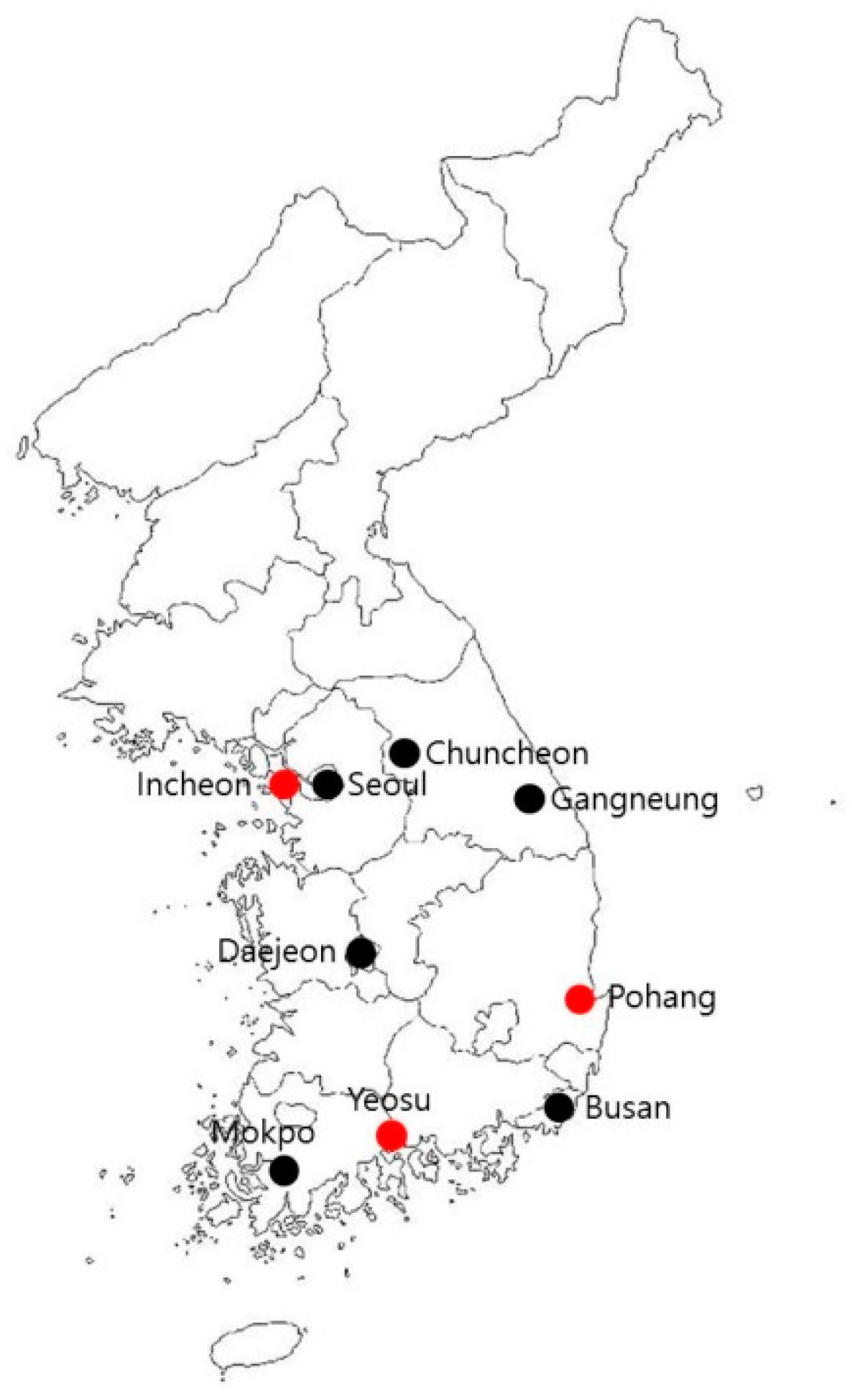
At present, the Korea Meteorological Administration (KMA) measures outdoor temperature and surface temperature at 95 observation points. However, ground temperature, which is an important factor for using geothermal heat, is measured at only nine observation points, at depths of 0.05, 0.1, 0.2, 0.3, 0.5, 1.0, 1.5, 3.0, and 5.0 m, including Seoul, as shown in Figure 1. For the other areas, it provides only outdoor and ground surface temperature. Ground temperature is greatly affected by ground surface temperature, which is often influenced by outdoor weather conditions [4,5]. In order to utilize ground temperature data in the field, it is measured in the vicinity of the target area. However, there are large variations not only in distance, but also in outer temperature and surface temperature depending on the target area; therefore, it is difficult to use the same ground temperature for different target areas.

Numerous studies are under way to predict ground temperature in various ways to utilize geothermal heat. Yener et al. [6] developed a model that uses a sine function with the amplitude of annual and daily average outdoor temperature and the amplitude of underground depths, and they predicted ground temperature in Turkey. Furthermore, they suggested a correlation among the ground temperature amplitudes by depth, the constant value between amplitude and annual average outdoor temperature, and the daily outdoor temperature amplitude. The study assumed that the amplitude of temperature wave decays exponentially with depth, which requires measurement of the amplitude of daily mean air temperature.

Tsilingiridis et al. [4] derived a regression equation according to ground depth by using the correlation with outdoor temperature to predict ground temperature at shallow depths in the northern Grecian region. They also proposed a quadratic equation to predict ground temperature at 1.0 and 1.5 m and reported that the predicted value had an accuracy of approximately 94.1% with respect to the measured value. However, the proposed six seasonal regression equations are only related to the local monthly average air temperature at one station in the northern Grecian region and cannot apply to predict ground temperature profiles of other regions.

Pouloupatis et al. [7] measured ground temperature by drilling boreholes at one point in Athalassa in Nicosia, which is in the lowlands of Cyprus, and at two points on the southern coast of Cyprus, in addition to installing thermocouples at different depths. The shallow zones in the three measured areas were reported to show temperature distributions depending on the seasonal cycle.

Popiel et al. [5] classified the ground into three zones: surface, shallow, and deep. The surface zone, located 1 m from the Earth’s surface, has a temperature distribution that is very sensitive to weather conditions, and the shallow zone, located 1–8 m (or up to 20 m) from the Earth’s surface, has a nearly constant temperature distribution that is closely related to the annual average air temperature. The deep zone is located 20 m or more from the surface of the Earth. The study reported that the amplitude indicating temperature change decreases as the depth from the surface increases. In addition, for the Poznan area, Popiel [8] used a cosine function to estimate the empirical coefficient of the time lag of ground temperature, thermal diffusivity, and surface temperature in bare and short-grass-covered areas, in addition to predicting the ground temperature and verifying its validity. However, the equation was developed with limited measurements at two stations in Poznan City, Poland. In addition, the constant values of thermal diffusivity and the phase lag of ground surface temperature wave were applied.

Jacovides et al. [9] analyzed a 74-year ground temperature measurement by using a Fourier technique to investigate surface and ground temperatures at different depths in Athens, Greece. They divided the study area into bare and short-grass-covered areas and estimated the ground temperature and the minimum/maximum values by depth and time through a statistical analysis. The study assumed homogeneous and constant physical properties of the ground. The Fourier coefficients of annual ground temperature and the amplitude of ground surface temperature wave were estimated from statistical fitting of the multiyear measurements.

Ouzzane [10] proposed a correlation model of outdoor temperature, wind speed, horizontal solar irradiation, and sky temperature to predict undisturbed ground temperature. He suggested a correlation coefficient of 0.98 or higher in 17 regions from Canada to Saudi Arabia with a simple correlation based on outdoor temperature, which is the most influential factor among the correlation factors.

Previous studies were performed to develop a statistical model with multiyear measurements using Fourier technique and regression models with the measured data of a limited period or stations predicting ground temperature profiles at certain depths. In addition, physical properties of the ground are assumed to be homogeneous and constant, and several models require complex parameters and field measurements to estimate ground temperature. Therefore, the results of the study are limited in predicting ground temperature profiles applying to other regions.

The use of direct or indirect earth-coupling techniques for building engineering applications requires knowledge of the ground temperature profile. Although ground temperature is assumed to be constant at certain depths, it varies especially near the surface. Knowledge of the annual variation of ground temperature by depth is necessary to predict the performance of earth-integrated engineering applications. These include ground heat exchanger applications [11,12], horizontal ground-source heat pump systems [13,14], earth-coupling solar chimney systems [15,16], and earth-tube systems [2,16,17,18].

Therefore, outdoor temperature, ground surface temperature, and thermal diffusivity are key factors in predicting ground temperature in order to examine the performance of the engineering applications. This study develops a regression equation by using the amplitude ratios of surface temperature and outdoor temperature provided by KMA, compares the results of prediction with measured data from Korea’s representative areas, and examines the validity of the developed regression equation with the measured data from two areas in Japan and the field-measured data.

2. Theoretical Considerations

The temperature field of a one-dimensional semi-infinite solid has certain values of thermal properties if there is no internal heat generation, as expressed by Equation (1):

$$\frac{\partial T}{\partial t}=\alpha \frac{{\partial }^{2}T}{\partial x^2}$$

(1)

where $x$ is the depth (m) below the surface of the Earth, $t$. is the time (s), and $\alpha$ is the thermal diffusivity (m²/s) divided by the thermal conductivity and the volumetric thermal capacity of the soil: $\alpha =k/\left(c·\rho \right)$. In Equation (1), ground temperature ($T$) depends on the variables of depth ($x$) and time ($t$), and if the boundary condition is $x=0$, it can be rewritten as follows:

$$T\left(x=0,t\right)=T_o+A_o·cos\left(\omega ·t\right)$$

(2)

where $T_o$ is the annual average ground temperature (°C) and $A_s$ is the ground surface temperature amplitude (°C); $\omega$ is the wavelength of the surface temperature, which is $2\mathsf{\pi }/365$. Kusuda et al. [19] corrected Equation (2) to Equation (3), assuming that the ground temperature was exposed to the periodically changing atmosphere over time:

$$T\left(x,t\right)=T_o+A_o·exp\left[-{\left(\frac{\omega }{2\alpha }\right)}^{1/2}·x\right]·cos\left[\omega ·\left(t-t_o\right)-{\left(\frac{\omega }{2\alpha }\right)}^{1/2}·x\right]$$

(3)

where $t_o$ represents the phase lag (day) of ground surface temperature.

3. Development of a Simplified Equation for Predicting Ground Temperature

3.1. Previous Experimental Equations

Baggs [20] changed Equation (3) to an empirical formula, Equation (4), to estimate the periodic ground temperature distribution on the Australian continent:

$$T\left(x,t\right)=\left(T_m\pm \Delta T_m\right)+1.07·k_v·A_{s}exp\left[-0.000316·x·{\left(\frac{1}{\alpha }\right)}^{\frac{1}{2}}\right]·cos\left[\frac{2\pi }{365}\left(t-t_o-0.01834·x·{\left(\frac{1}{\alpha }\right)}^{\frac{1}{2}}\right)\right]$$

(4)

where $x$ is the underground depth (m), $t$ is the time of year from 1 January (day), $T_m$ is the annual average outdoor temperature (°C), $T_g$ is the average ground temperature below the shallow zone (°C), $\Delta T_m$ = $T_g-T_m$ (°C), $k_v$ is the vegetation shade factor, $A_s$ is the annual air temperature amplitude (°C), $\alpha$ is the annual average soil thermal diffusivity (m²/s), and $t_o$ is the phase lag of ground surface temperature wave (day).

Popiel [5] modified Equation (4) to Equation (5) by setting $\alpha$ and $A_s$ as constant values of 55 × 10⁻⁸ [m²/s] and 11.6 K to use them in the Northern Hemisphere:

$$T\left(x,t\right)=\left(T_m+\Delta T_m\right)-1.07·k_v·A_{s}exp\left[-0.000316·x·{\left(\frac{1}{\alpha }\right)}^{\frac{1}{2}}\right]·cos\left[\frac{2\pi }{365}\left(t-t_o-0.01834·x·{\left(\frac{1}{\alpha }\right)}^{\frac{1}{2}}\right)\right]$$

(5)

In addition, the experimental results were compared with the empirical results obtained using Equation (5) for Poznan City’s “car park” and “lawn” [8]. In order to predict ground temperature using Equation (5), factors such as annual average ground surface temperature, amplitude of the annual average ground surface temperature wave, underground depth, ground thermal diffusivity, and phase lag of ground surface temperature wave are required.

3.2. Development of a Simplified Equation

The estimation equation (Equation (6)) with the modification of Equation (4) is utilized to predict the depth-specific ground temperature by introducing model coefficients such as a temperature coefficient $a$ (°C), an apparent ground temperature below a shallow zone, an apparent soil thermal diffusivity $\alpha$, and the phase lag of ground surface temperature wave $t_o$, which are empirical coefficients. To overcome the previous models’ requirement for complex model parameters and field measurements, the model coefficients of the developed equation are estimated from the monthly outdoor air and ground surface temperature for a year, which are easily obtained from local weather stations.

$$T\left(x,t\right)=a-1.07·k_v·A_{s}exp\left[-0.000316·x·{\left(\frac{1}{\alpha }\right)}^{\frac{1}{2}}\right]·cos\left[\frac{2\pi }{365}\left(t-t_o-0.01834·x·{\left(\frac{1}{\alpha }\right)}^{\frac{1}{2}}\right)\right]$$

(6)

3.3. Determination of Model Coefficients

The amplitude of outdoor temperature wave affects the amplitude of ground surface temperature wave. Therefore, the correlation between the two measured temperature amplitudes affects the variation of ground temperature. In this study, to develop a simplified estimation equation for ground temperature using the amplitude ratio of surface and outdoor temperature waves, we used the monthly averages of ground surface and outdoor temperature at nine measurement points from 2006 to 2015, which are provided by KMA.

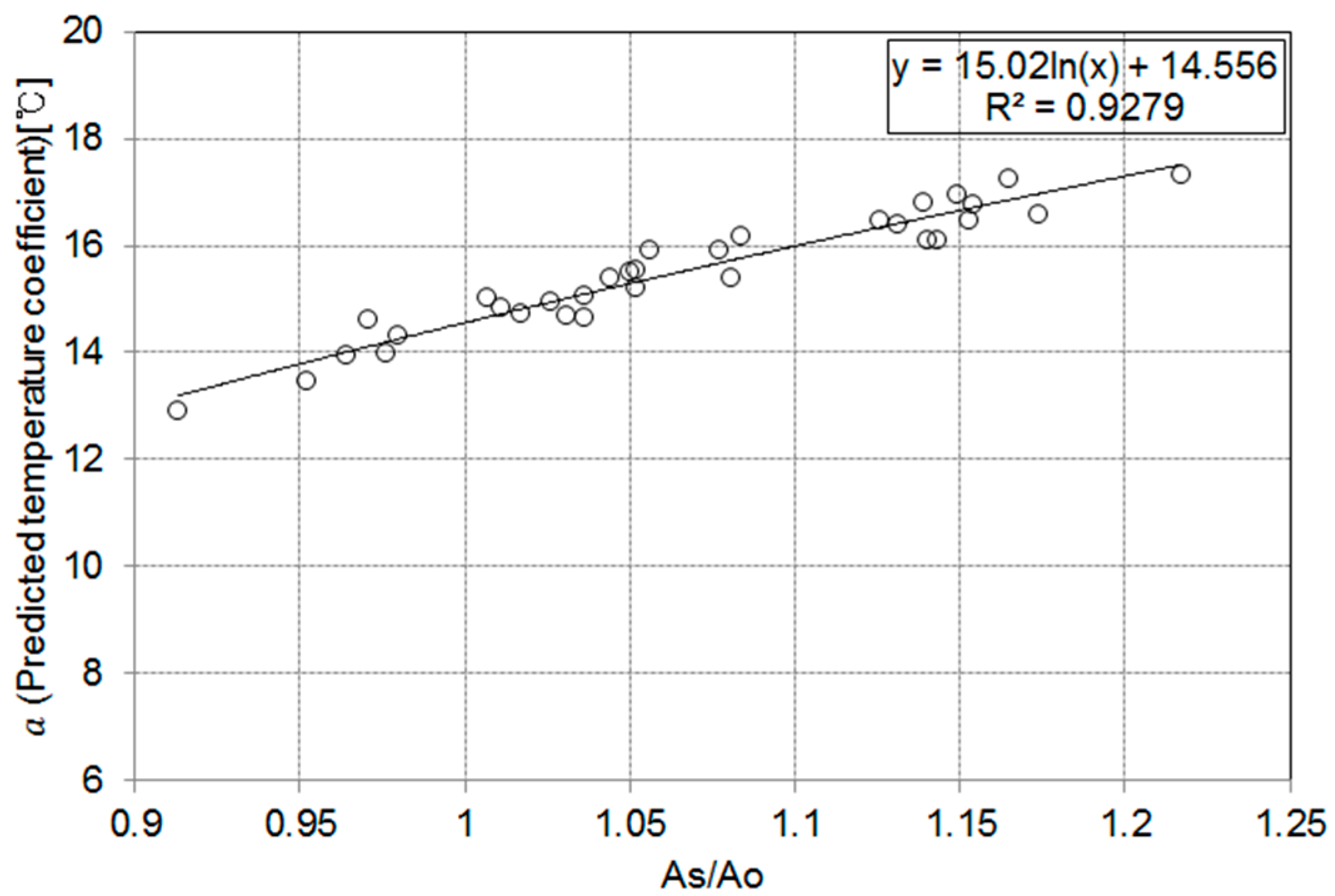
First, a regression analysis was performed using the amplitude ratio ($A_s/A_o$) of ground surface and outdoor temperature waves provided by KMA to predict a temperature coefficient. The temperature coefficient $a$ can be obtained by the regression equation (Equation (7)) with a coefficient of determination $R^2$ of 0.928 based on the amplitude ratio ($A_s/A_o$), as shown in Figure 2.

$$a=15.02\times \ln \left(\frac{A_s}{A_o}\right)+14.556$$

(7)

The vegetation shade factor $k_v$ proposed by Baggs [20] has a large value in the case of high solar radiation on bare ground. Popiel revised this value to the range of 1.2–1.45 for bare ground and 0.9 for short-grass-covered ground [5]. In the field experiment, the average value of the vegetation shade factor proposed by Popiel, 1.1, was applied because the study area has both bare and short-grass-covered areas.

Kusuda [19] and Horton [21] measured thermal diffusivity over 18 years in Edinburgh, Scotland. They reported that the measured thermal diffusivity was in good agreement with the value predicted using the amplitude equation (Equation (8)) and that there was a linear relationship between the depth and amplitude of the ground. Therefore, Equation (8) estimates apparent soil thermal diffusivity by depth:

$$\alpha =\left(\frac{\omega }{2}\right){\left[\frac{x_2-x_1}{\ln \left(\frac{A_1}{A_2}\right)}\right]}^2$$

(8)

where A₁ and A₂ represent the amplitudes at underground depths x₁ and x₂, respectively.

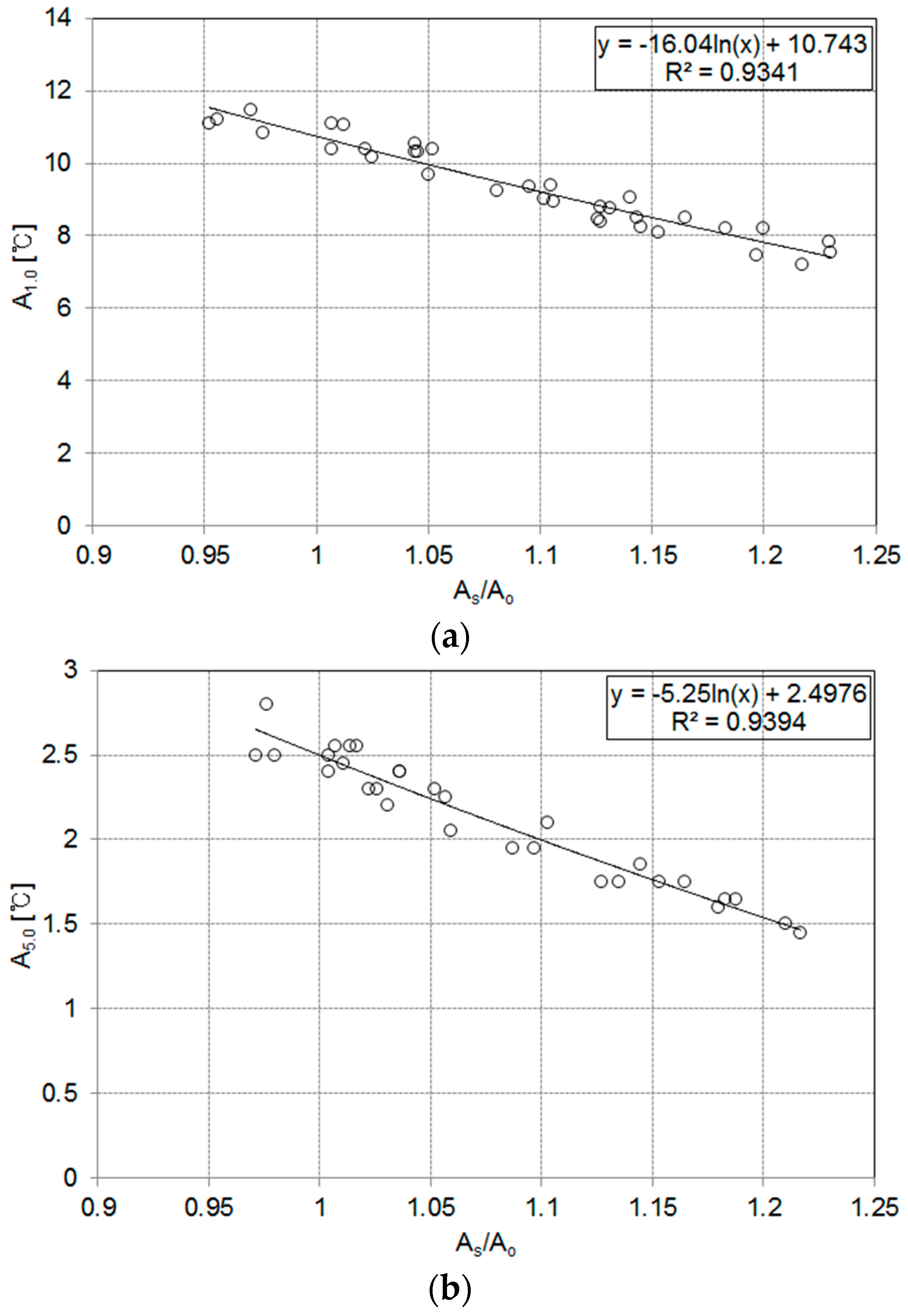
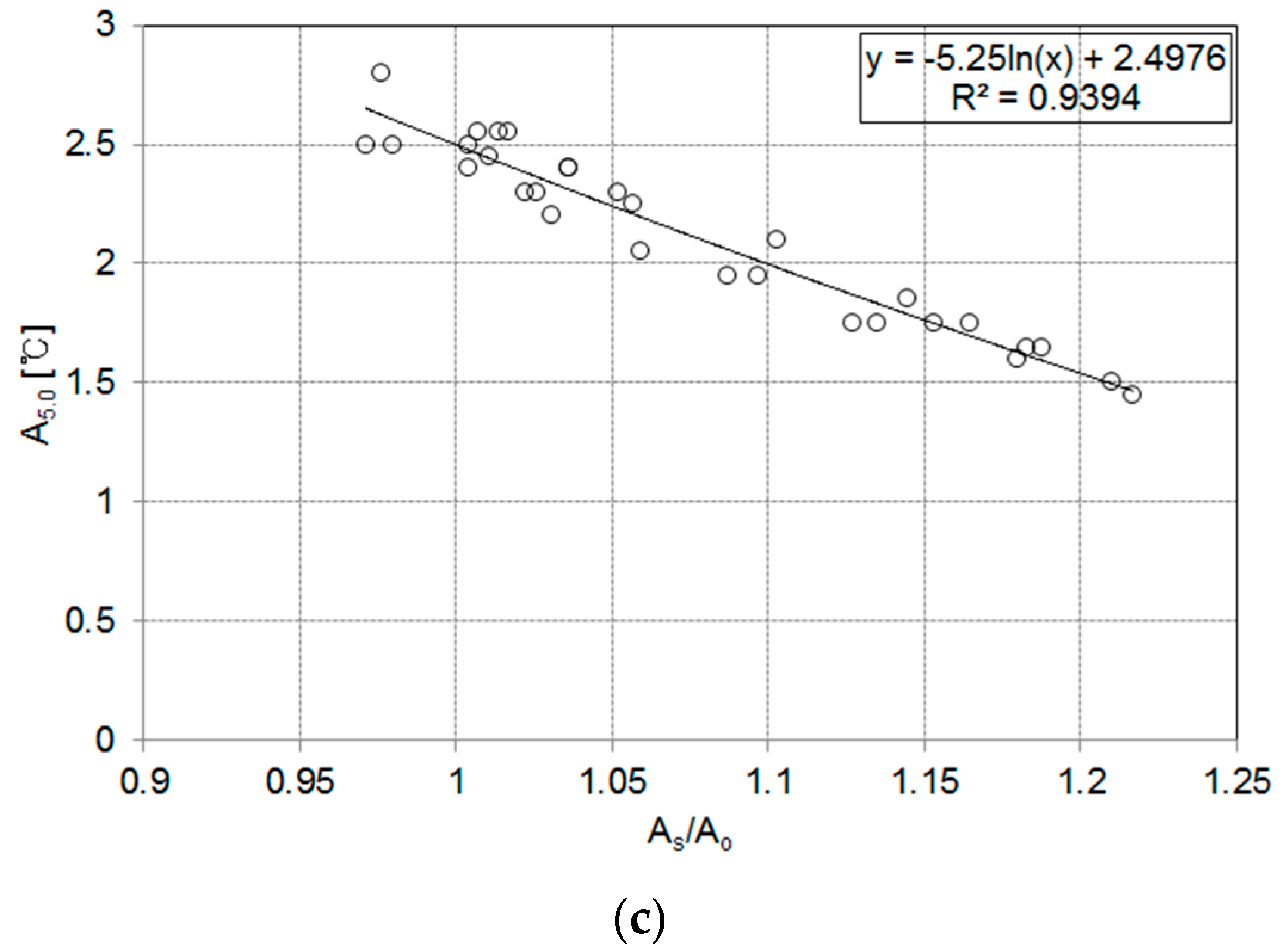
The amplitude at each underground depth is predicted by a regression analysis using the amplitude ratio ($A_{\mathrm{s}}/A_o$). As shown in Figure 3, the amplitude coefficients of determination $R^2$ are 0.934, 0.932, and 0.939 at depths of 1, 3, and 5 m, respectively, indicating a significant correlation. The estimation formula is summarized as Equation (9):

Amplitude at a depth of 1.0 m:

$$A_{1.0}=-16.04ln(A_s/A_o)+10.743$$

(9a)

Amplitude at a depth of 3.0 m:

$$A_{3.0}=-7.473ln(A_s/A_o)+4.9083$$

(9b)

Amplitude at a depth of 5.0 m:

$$A_{5.0}=-5.25ln(A_s/A_o)+2.4976$$

(9c)

where $A$ is the amplitude by underground depth, $A_s$ is the ground surface temperature amplitude, and $A_o$ is the outdoor temperature amplitude.

We compared the amplitude at each underground depth provided by KMA with the value predicted using Equation (9). The measured and predicted values are 9.41 °C and 9.42 °C at an underground depth of 1.0 m, 4.49 °C and 4.29 °C at an underground depth of 3.0 m, and 2.19 °C and 2.07 °C at an underground depth of 5.0 m, respectively. Most of the amplitudes obtained using the regression equations in Equation (9) are within the amplitude range of the measured data. It can be seen that amplitude decreases as depth increases, which is consistent with the results of previous studies [7,8,11,20].

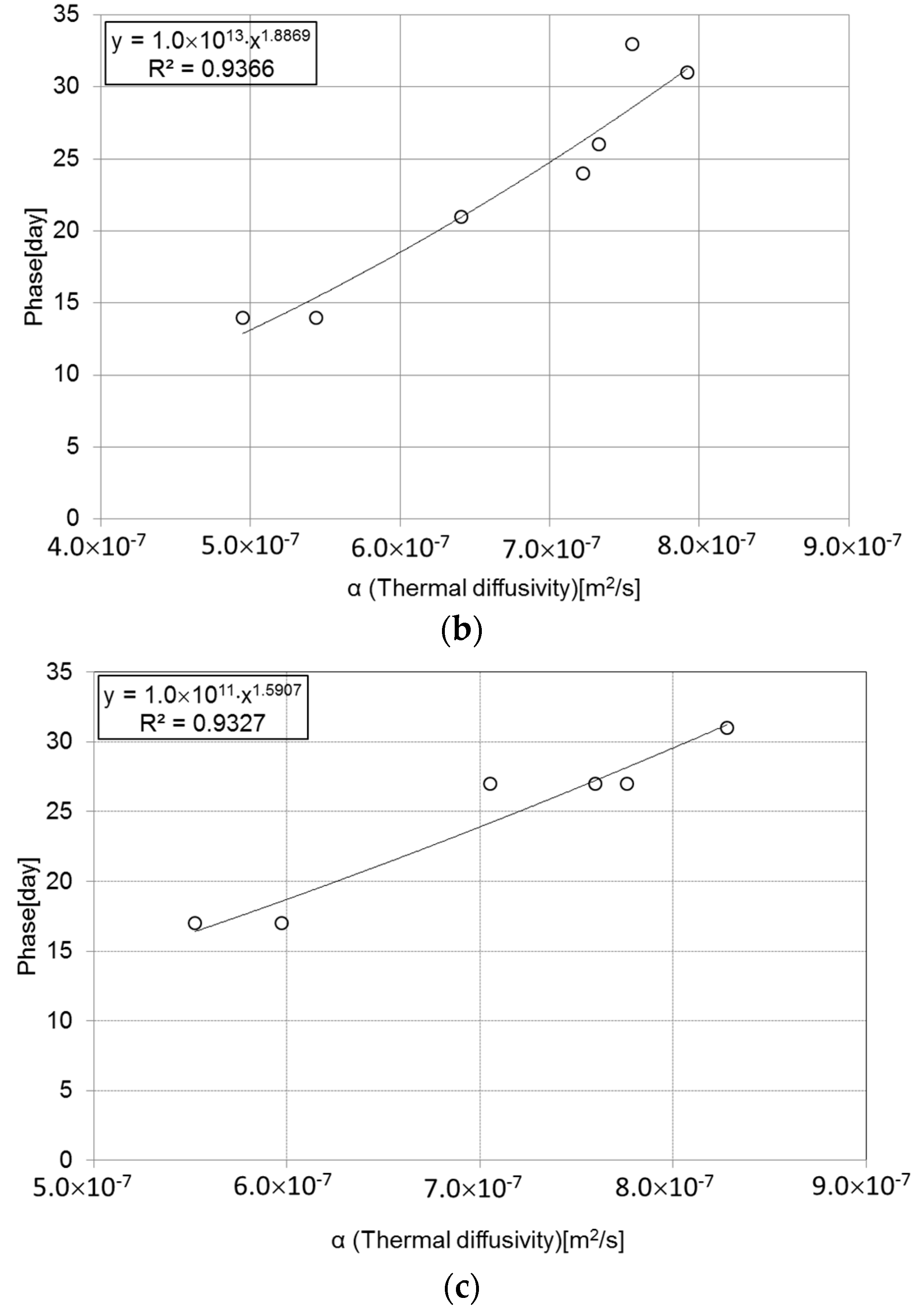
In Equation (6), the apparent soil thermal diffusivity is related to time, and the phase lag of ground surface temperature wave varies with time. Therefore, the phase lag can be derived with the regression equation based on the apparent soil thermal diffusivity, as expressed by Equation (10). The coefficients of determination at depths of 1.0, 3.0, and 5.0 m are 0.975, 0.937, and 0.933, respectively, with a confidence level of 95%, as provided in Figure 4.

$$t_{o,1.0m}=\mathrm{36,879}\times {\alpha }_{1.0}^{0.5169}$$

(10a)

$$t_{o,3.0m}=1\times {10}^{13}\times {\alpha }_{3.0}^{1.8869}$$

(10b)

$$t_{o,5.0m}=1\times {10}^{11}\times {\alpha }_{5.0}^{1.5907}$$

(10c)

4. Results

4.1. Comparative Analysis of Ground Temperature Distribution in Korea

Korea is geographically surrounded by water on three sides. As shown in Figure 1, among the nine points that have been measured thus far by KMA, the underground temperature distribution was analyzed at three locations: Pohang on the east coast, Incheon on the west coast, and Yeosu on the south coast. Ground temperatures at depths of 1, 3, and 5 m are calculated using Equation (6) with the developed regression equations, the temperature coefficient of Equation (7), the apparent soil thermal diffusivity of Equation (8), and the phase lag of ground surface temperature wave of Equation (10), and compared with the measured data provided by KMA.

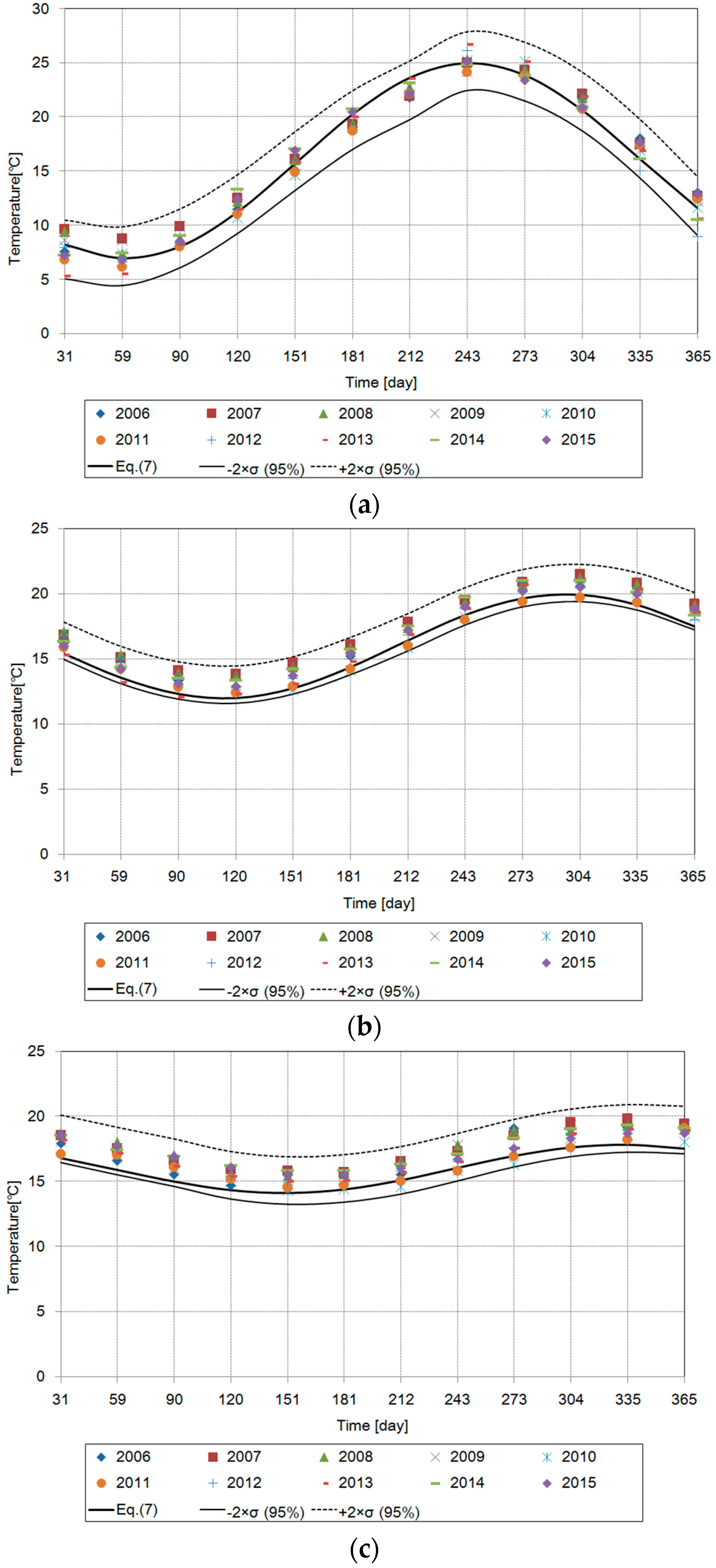
4.1.1. Pohang

Pohang is located in the southern part of the eastern coast. The daily average outdoor temperature over 10 years is in the range of 2.1–26.2 °C, and the ground surface temperature is in the range of 1.7–29.8 °C. The amplitude ratio ($A_{\mathrm{s}}/A_o)$ of annual ground surface temperature and annual outdoor temperature over 10 years, provided by KMA, is 1.17, and $A_{\mathrm{s}}$ is 14.80 °C.

Table 1. Coefficients for estimating ground temperature in Pohang.

${\mathit{A}}_{\mathbf{s}} \left({}^{°}\mathrm{C}\right)$	${\mathit{A}}_{\mathit{o}} \left({}^{°}\mathrm{C}\right)$	$\mathit{a} \left({}^{°}\mathrm{C}\right)$	${\mathit{A}}_{\mathit{s}}/{\mathit{A}}_{\mathit{d}\mathit{e}\mathit{p}\mathit{t}\mathit{h}}$		Phase Lag (Day)
			$A_{\mathrm{s}}/A_{1.0}$	1.86	$t_{o,1.0m}$	16.6
14.80	12.70	16.92	$A_{\mathrm{s}}/A_{3.0}$	3.94	$t_{o,3.0m}$	13.9
			$A_{\mathrm{s}}/A_{5.0}$	9.28	$t_{o,5.0m}$	14.6

lists the coefficients used in the regression equation to predict underground temperature.

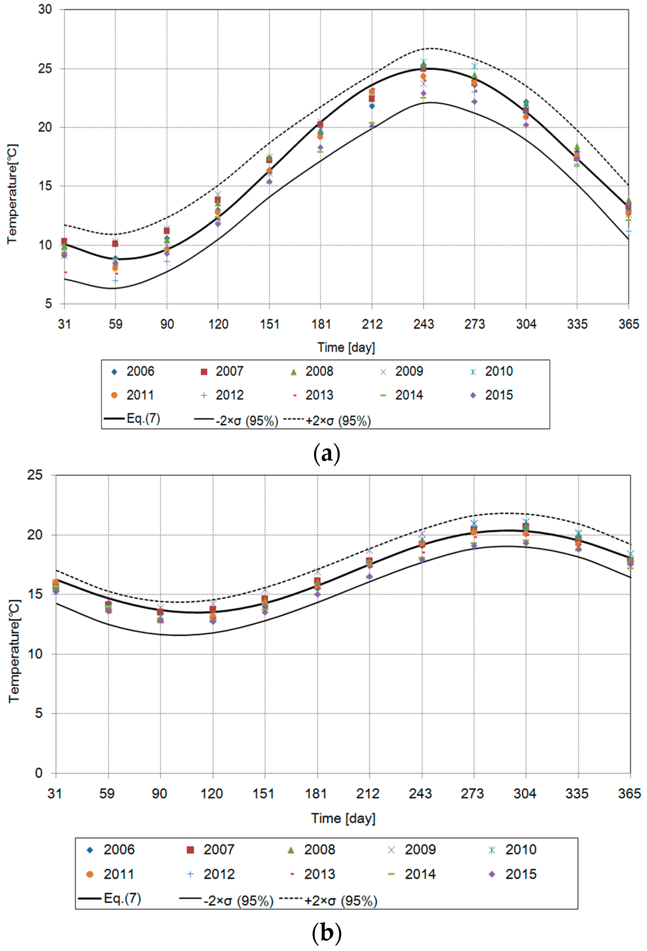
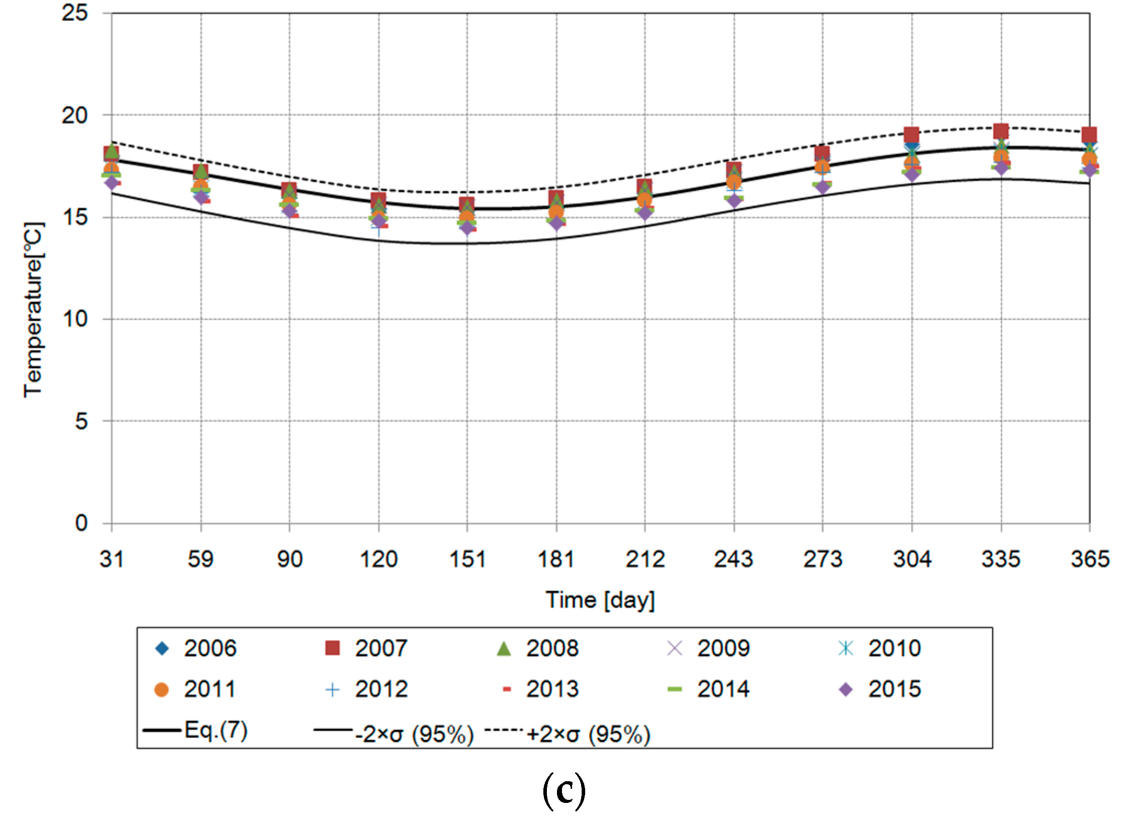
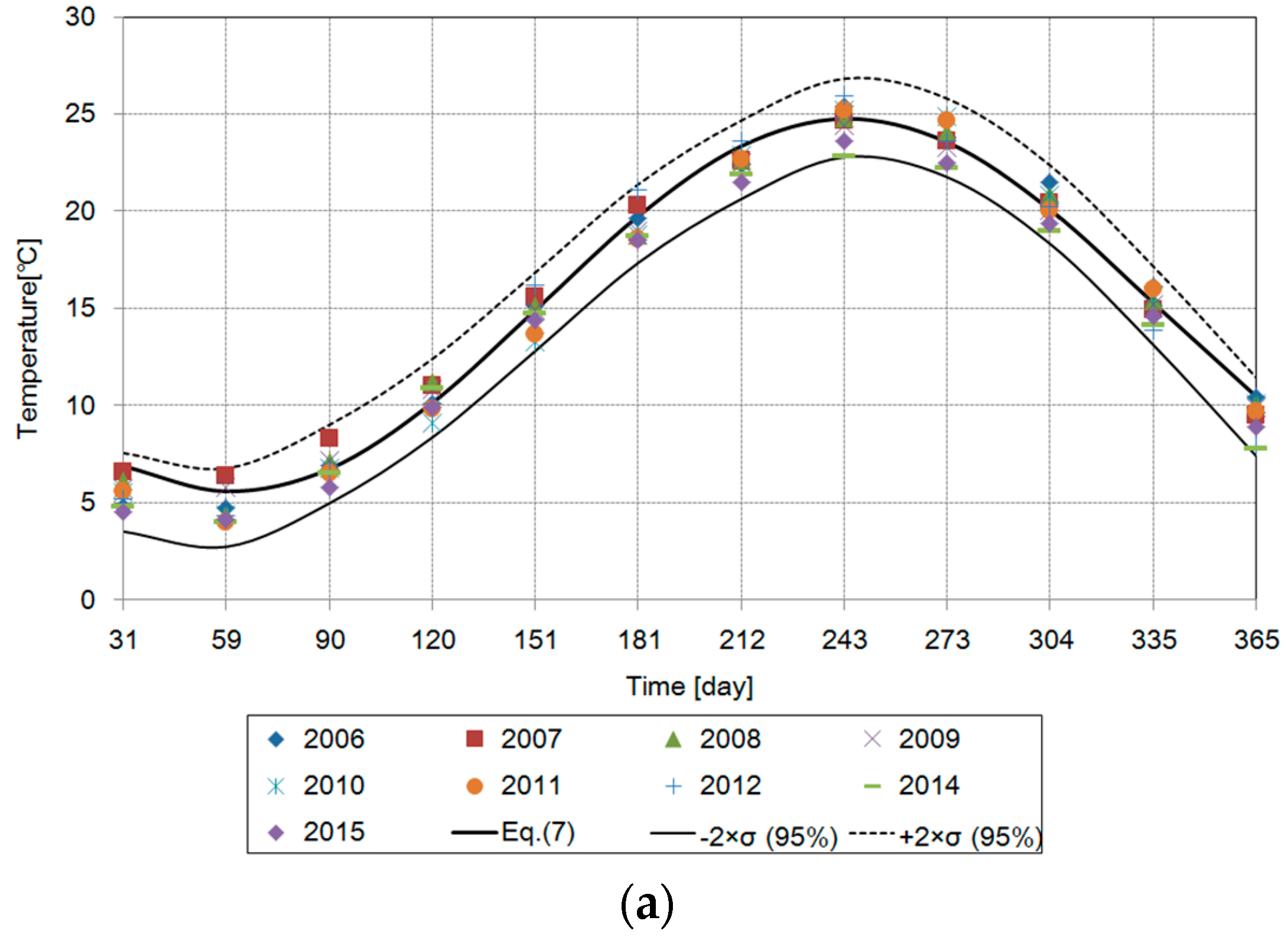
The monthly measured and predicted ground temperature distributions were compared for 10 years at depths of 1.0, 3.0, and 5.0 m in Pohang, as shown in Figure 5. At a depth of 1 m, the measured ground temperature ranges from 8.6 °C to 24.4 °C over 10 years, with a standard deviation (σ) of 1.15 °C, and the predicted values calculated from Equation (6) are distributed from 8.8 °C to 25.0 °C. The ground temperature distribution for a depth of 3.0 m is in the range of 13.0–20.4 °C, and the calculated values are in the range of 13.5–20.3 °C. The average distribution of ground temperature at a depth of 5 m is in the range of 15.0–18.5 °C, and the calculated values are in the range of 15.4–18.4 °C. These results demonstrate that there is good agreement between the measured and calculated values of ground temperature at each depth, with similar trends of temperature distribution. The ground temperature estimated from the regression equation is within the range of $\pm 2\sigma$ (95% confidence level) of the ground temperature provided by KMA.

4.1.2. Incheon

Incheon is a coastal city in the northern part of the western coast. The daily average outdoor temperature over 10 years is in the range of 1.7–25.7 °C, and the surface temperature is in the range of −2.5–30.6 °C. The annual average surface temperature amplitude ($A_{\mathrm{s}}$) is 14.38 °C over 10 years, and the ratio of amplitude ratio ($A_{\mathrm{s}}/A_o)$ to outdoor temperature amplitude ($A_o)$ is 1.04.

The coefficients applied to the regression equation are listed in

Table 2. Coefficients for estimating ground temperature in Incheon, Korea.

${\mathit{A}}_{\mathbf{s}} \left({}^{°}\mathrm{C}\right)$	${\mathit{A}}_{\mathit{o}} \left({}^{°}\mathrm{C}\right)$	$\mathit{a} \left({}^{°}\mathrm{C}\right)$	${\mathit{A}}_{\mathit{s}}/{\mathit{A}}_{\mathit{d}\mathit{e}\mathit{p}\mathit{t}\mathit{h}}$		Phase Lag (Day)
			$A_{\mathrm{s}}/A_{1.0}$	1.45	$t_{o,1.0m}$	25.7
14.38	13.80	15.18	$A_{\mathrm{s}}/A_{3.0}$	3.33	$t_{o,3.0m}$	30.1
			$A_{\mathrm{s}}/A_{5.0}$	6.56	$t_{o,5.0m}$	23.4

, and Figure 6 shows the ground temperature distribution by underground depth. The ground temperature distribution at a depth of 1.0 m is in the range of 4.8–24.8 °C, and the calculated values are in the range of 5.6–24.8 °C. The measured values at a depth of 3.0 m are in the range of 10.9–19.5 °C, and the calculated values are in the range of 11.0–19.4 °C. The measured temperature at a depth of 5.0 m is in the range of 12.8–17.1 °C, and the calculated ground temperature is in the range of 13.1–17.2 °C. The ground temperature in Incheon estimated from the regression equation is within $\pm 2\sigma$ (95% confidence level) of the ground temperature provided by KMA.

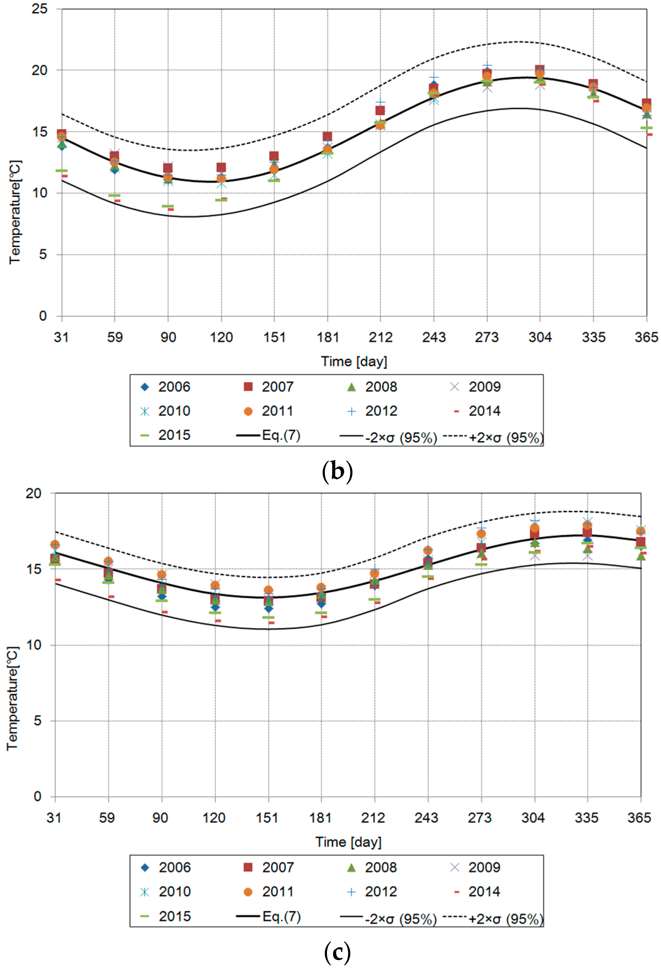
4.1.3. Yeosu

Yeosu is a coastal city in the southern part of Korea. The daily average outdoor temperature over 10 years is in the range of 2.5–25.9 °C, and the surface temperature is in the range of −1.9–27.6 °C. The amplitude ratio ($A_{\mathrm{s}}/A_o)$ over 10 years provided by KMA is 1.10, and the annual average surface temperature amplitude ($A_{\mathrm{s}}$) is 13.30 °C. The coefficients applied to the regression equation are listed in

Table 3. Coefficients for estimating the ground temperature in Yeosu, Korea.

${\mathit{A}}_{\mathbf{s}} \left({}^{°}\mathrm{C}\right)$	${\mathit{A}}_{\mathit{o}} \left({}^{°}\mathrm{C}\right)$	$\mathit{a} \left({}^{°}\mathrm{C}\right)$	${\mathit{A}}_{\mathit{s}}/{\mathit{A}}_{\mathit{d}\mathit{e}\mathit{p}\mathit{t}\mathit{h}}$		Phase Lag (Day)
			$A_{\mathrm{s}}/A_{1.0}$	1.45	$t_{o,1.0m}$	26.8
13.30	12.10	15.96	$A_{\mathrm{s}}/A_{3.0}$	3.33	$t_{o,3.0m}$	32.1
			$A_{\mathrm{s}}/A_{5.0}$	6.44	$t_{o,5.0m}$	22.6

, and the monthly measured and predicted ground temperature distributions are compared in Figure 7 at depths of 1.0, 3.0, and 5.0 m.

The average temperature at a depth of 1.0 m is in the range of 7.1–25.2 °C over 10 years with a standard deviation (σ) of 1.36 °C, and the temperature distribution predicted from Equation (6) is in the range of 7.1–25.2 °C. The measured underground temperature distribution at a depth of 3.0 m is in the range of 13.0–20.8 °C with a standard deviation (σ) of 0.72 °C, and the temperature calculated from Equation (6) is in the range of 12.0–19.9 °C. Additionally, the measured and calculated values at a depth of 5.0 m are in the range of 15.1–19.1 °C with standard deviations (σ) of 0.91 °C and 14.1–17.8 °C, respectively.

4.2. Validation with Ground Temperature Distribution in Japan

The developed regression equation was examined for its validity at two locations, Tokyo and Nagasaki in Japan. The monthly averages of ground surface temperature and outdoor temperature in Tokyo were measured from 1945 to 1954 with different periods by depth and in Nagasaki from 1940 to 1949, which are provided by the Japan Meteorological Administration (JMA). The ground temperatures at depths of 1, 3, and 5 m are calculated using Equation (6) with the model coefficients, the temperature coefficient, the apparent soil thermal diffusivity, and the phase lag of ground surface temperature wave, and they are compared with the measured data provided by JMA.

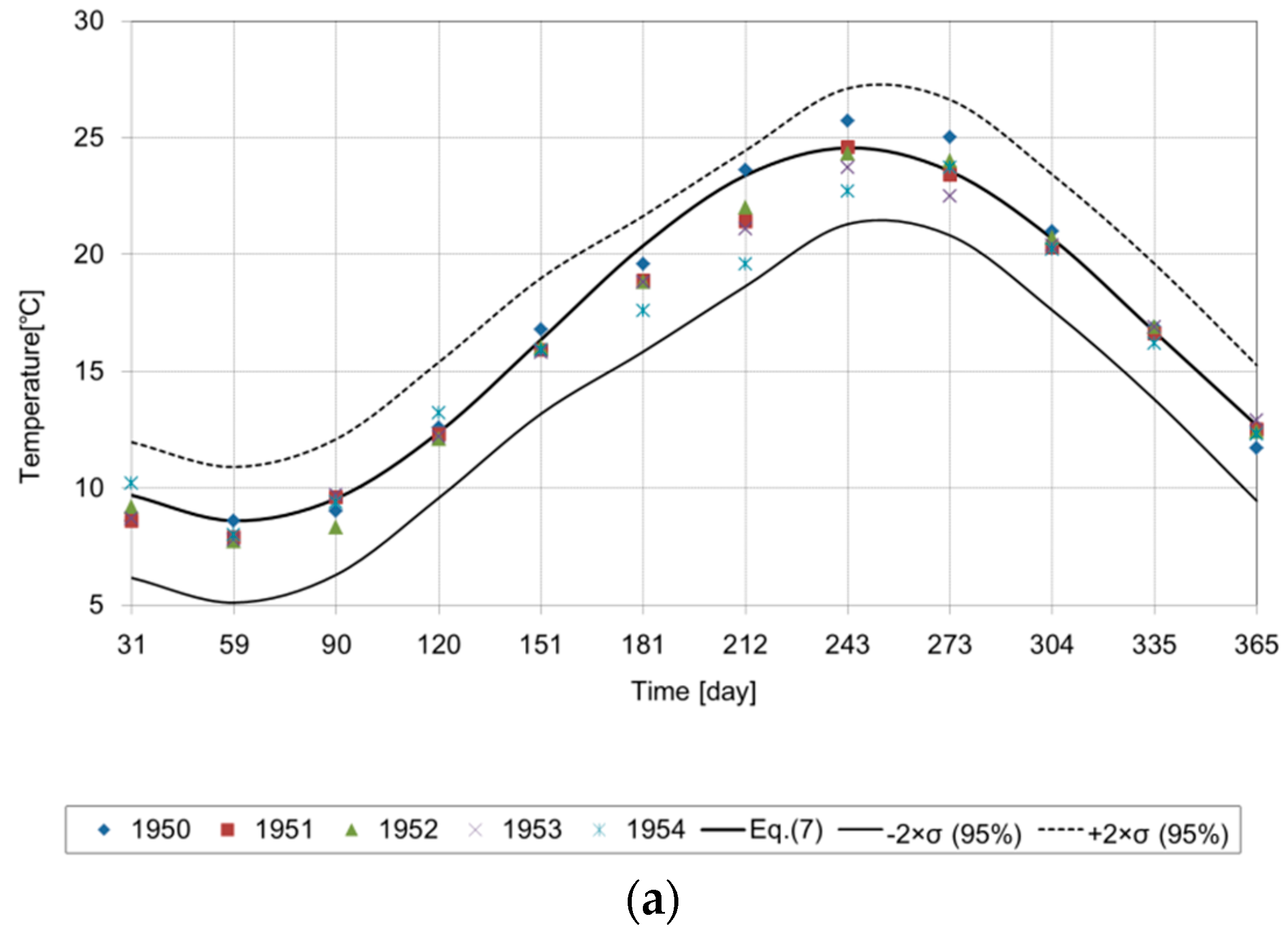
4.2.1. Tokyo

Tokyo is located at latitude 38° N and longitude 138° E. The monthly average outdoor temperature over 10 years is in the range of 3.8–26.5 °C, and the ground surface temperature is in the range of 3.4–29.5 °C. The amplitude ratio ($A_{\mathrm{s}}/A_o)$ of the annual ground surface temperature and annual outdoor temperature over 10 years is 1.145.

Table 4. Coefficients for estimating the ground temperature in Tokyo, Japan.

${\mathit{A}}_{\mathbf{s}} \left({}^{°}\mathrm{C}\right)$	${\mathit{A}}_{\mathit{o}} \left({}^{°}\mathrm{C}\right)$	$\mathit{a} \left({}^{°}\mathrm{C}\right)$	${\mathit{A}}_{\mathit{s}}/{\mathit{A}}_{\mathit{d}\mathit{e}\mathit{p}\mathit{t}\mathit{h}}$		Phase Lag (Day)
			$A_{\mathrm{s}}/A_{1.0}$	1.55	$t_{o,1.0m}$	20.9
13.22	11.56	16.59	$A_{\mathrm{s}}/A_{3.0}$	3.42	$t_{o,3.0m}$	24.1
			$A_{\mathrm{s}}/A_{5.0}$	7.55	$t_{o,5.0m}$	23.5

lists the coefficients used in the regression equation to predict underground temperature.

The monthly measured and predicted ground temperature distributions in Tokyo were compared by depth, as shown in Figure 8. At a depth of 1 m, the measured ground temperature ranges from 8.0 °C to 24.2 °C over 5 years with a standard deviation (σ) of 1.45 °C, and the predicted values calculated from Equation (6) are distributed from 8.6 °C to 24.6 °C. The ground temperature distribution for a depth of 3.0 m is in the range of 13.0–20.2 °C, and the calculated values are in the range of 13.1–20.2 °C. The average distribution of ground temperature at a depth of 5 m is in the range of 13.6–18.8 °C, and the calculated values are in the range of 15.0–18.2 °C. These results demonstrate good agreement between the measured and calculated values of ground temperature with similar trends of temperature distribution.

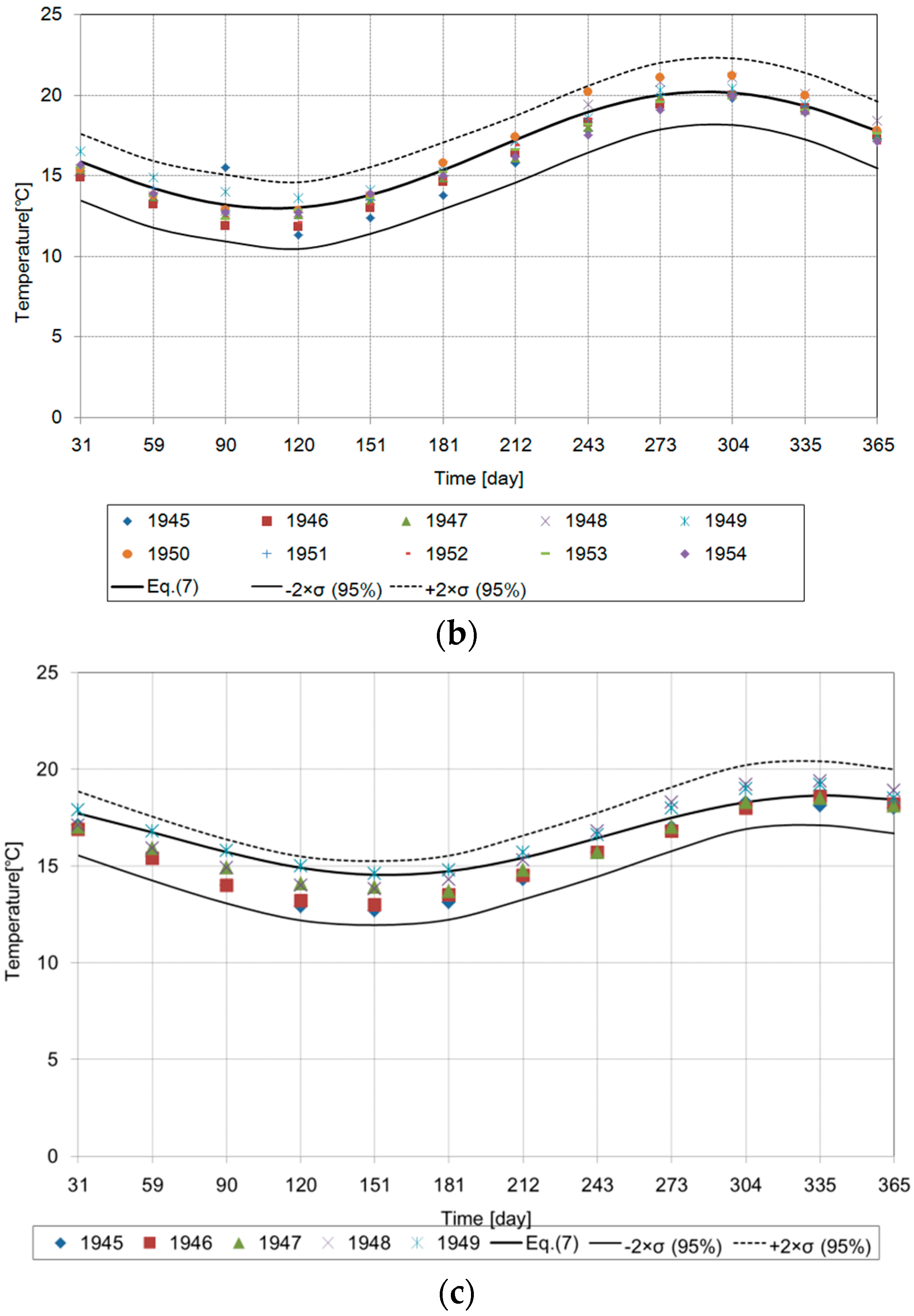
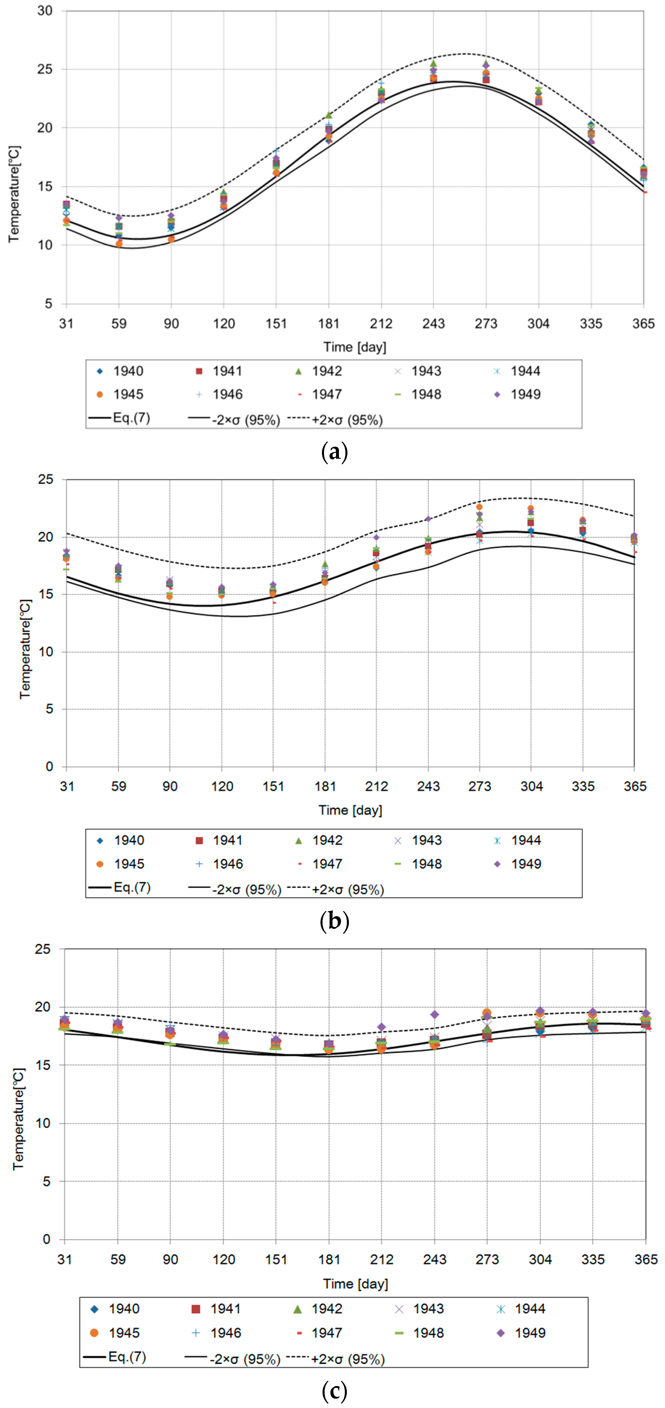
4.2.2. Nagasaki

Nagasaki is located on the northwest coast of the island of Kyushu. The monthly average outdoor temperature over 10 years is in the range of 4.2–27.1 °C, and the ground surface temperature is in the range of 6.5–31.4 °C. The amplitude ratio ($A_{\mathrm{s}}/A_o)$ over 10 years is 1.20.

Table 5. Coefficients for estimating ground temperature in Nagasaki, Japan.

${\mathit{A}}_{\mathbf{s}} \left({}^{°}\mathrm{C}\right)$	${\mathit{A}}_{\mathit{o}} \left({}^{°}\mathrm{C}\right)$	$\mathit{a} \left({}^{°}\mathrm{C}\right)$	${\mathit{A}}_{\mathit{s}}/{\mathit{A}}_{\mathit{d}\mathit{e}\mathit{p}\mathit{t}\mathit{h}}$		Phase Lag (Day)
			$A_{\mathrm{s}}/A_{1.0}$	1.66	$t_{o,1.0m}$	18.3
12.8	10.71	17.24	$A_{\mathrm{s}}/A_{3.0}$	3.51	$t_{o,3.0m}$	19.4
			$A_{\mathrm{s}}/A_{5.0}$	8.65	$t_{o,5.0m}$	19.6

lists the coefficients used in the regression equation and Figure 9 compares the monthly measured and predicted ground temperature distributions.

The measured ground temperature is in the range of 11.2–24.8 °C with a standard deviation (σ) of 0.69 °C at a depth of 1 m, and the predicted values are distributed from 10.1 °C to 24.4 °C. The ground temperature distribution at a depth of 3.0 m is in the range of 15.2–21.3 °C, and the calculated values are in the range of 14.1–20.4 °C. The measured and calculated ground temperature is in the range of 16.7–18.8 °C and 15.9–18.6 °C at a depth of 5 m, respectively. The estimated ground temperature is within the range of $\pm 2\mathsf{\sigma }$ (95% confidence level) of the ground temperature.

4.3. Validation with Experimental Measurements

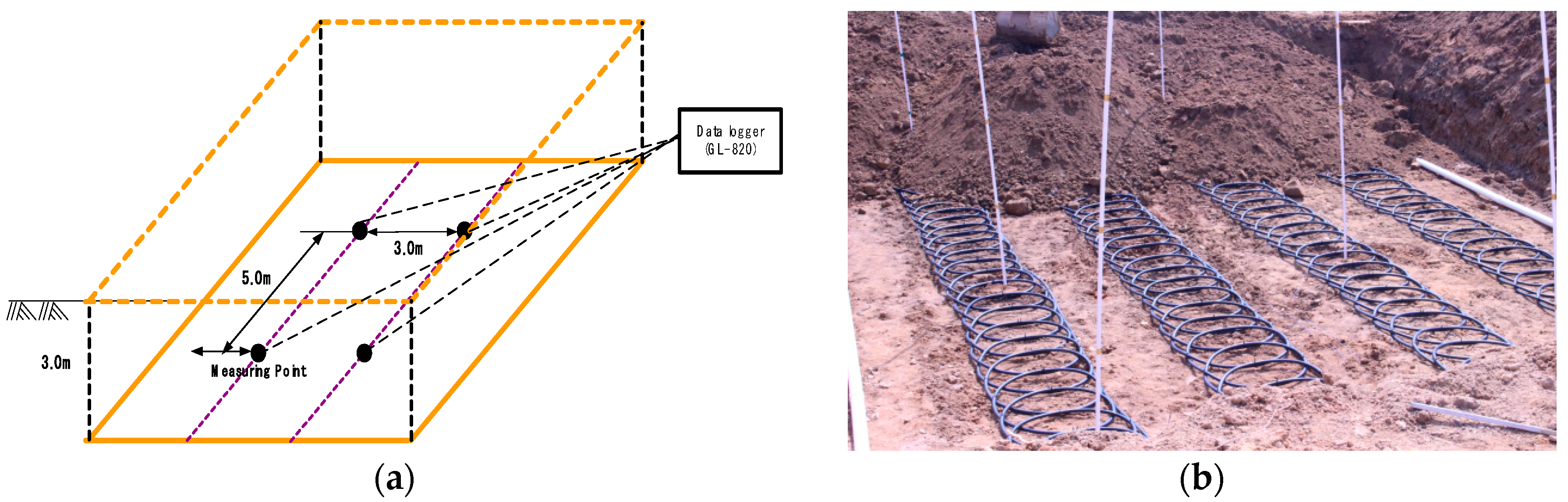
Changwon is located close to Busan, which is on the southern coast. KMA provides only outdoor and ground surface temperatures for Changwon. In order to verify the developed simplified equation, temperature was measured at a depth of 3 m for one year from 1 January to 31 December, 2017, and the results were compared with the predicted values.

A K-type thermocouple was installed at a depth of 3 m, where an earth tube was buried. The hourly ground temperature was recorded and daily average temperature was calculated for comparison with the predicted value. The coefficients applied to the regression equation are listed in

Table 6. Coefficients for estimating ground temperature in Changwon, Korea.

${\mathit{A}}_{\mathbf{s}} \left({}^{°}\mathrm{C}\right)$	${\mathit{A}}_{\mathit{o}} \left({}^{°}\mathrm{C}\right)$	$\mathit{a} \left({}^{°}\mathrm{C}\right)$	${\mathit{A}}_{\mathit{s}}/{\mathit{A}}_{\mathit{d}\mathit{e}\mathit{p}\mathit{t}\mathit{h}}$		Phase Lag (Day)
14.02	12.12	16.75	$A_{\mathrm{s}}/A_{3.0}$	3.82	$t_{o,3.0m}$	17.0

. Figure 10 illustrates the measured points and equipment installed at the field.

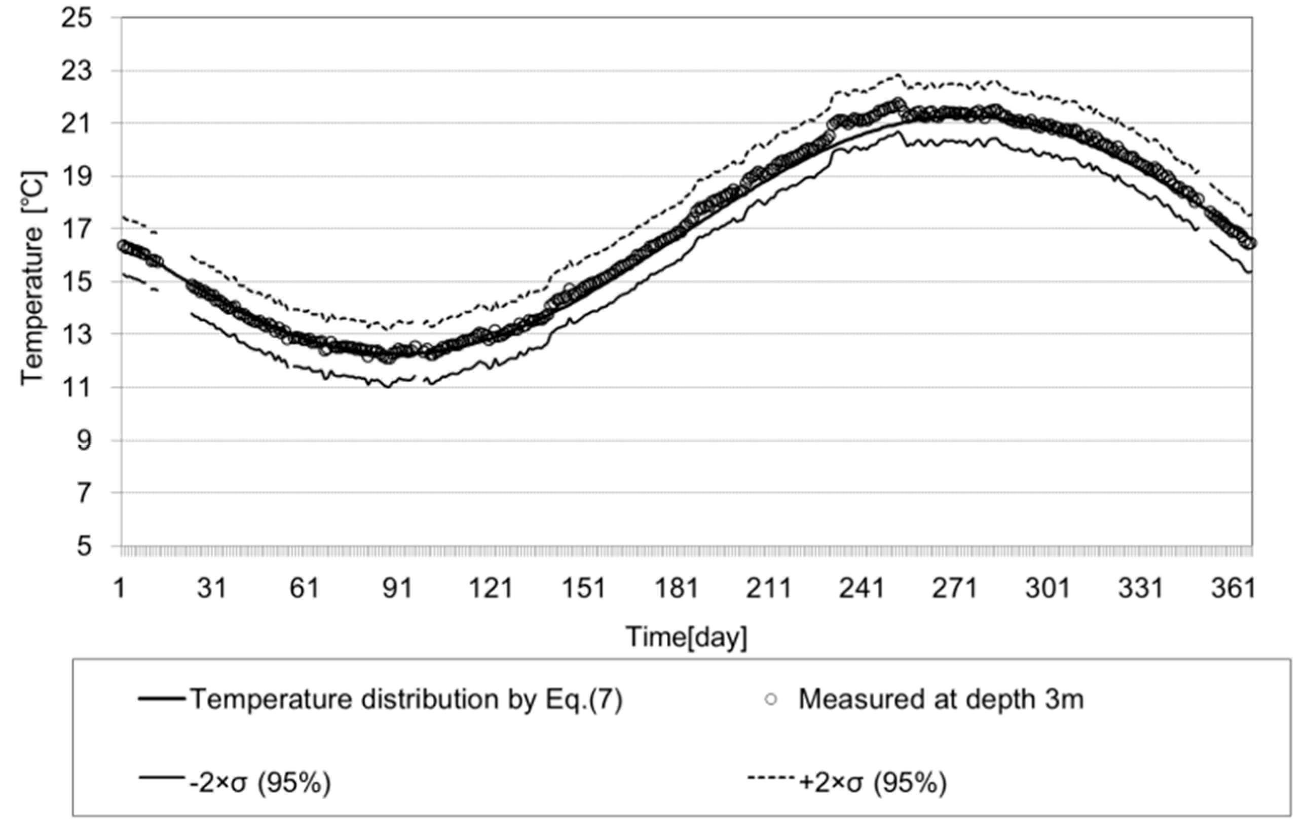
The monthly outdoor and ground surface temperatures over 10 years from 2006 to 2015 provided by KMA are in the range of 2.5–26.4 °C and 2.1–29.5 °C, respectively. The coefficients used in Equation (6) are listed at Table 6; the amplitude ($A_{\mathrm{s}}$) of ground surface temperature is 14.0 °C, and the amplitude ratio ($A_{\mathrm{s}}/A_o)$ of outdoor temperature is 1.16. Figure 11 illustrates and compares the hourly ground temperatures at a depth of 3 m between the regression equation and field measurements in Changwon.

The ground temperature was in the range of 12.4–21.1 °C, and the annual average ground temperature was 16.7 °C. The predicted ground temperature distribution is in the range of 12.5–21.4 °C, and the annual average temperature is 16.9 °C. The predicted temperatures are almost the same as the experimental values. Therefore, it is concluded that the proposed simplified equation can be used to predict ground temperature by depth in Korea.

5. Conclusions

KMA provides data on outdoor and ground surface temperatures. However, underground temperature by depth is measured for limited areas. Therefore, it is very difficult to predict underground temperature in the field. Accordingly, this study aimed to investigate the data on underground temperature by depth provided by KMA and to develop a simplified regression equation using the amplitude ratios of ground surface and outdoor temperatures to predict the underground temperature distributions throughout the country. The estimated annual variation of ground temperature at various depths can be utilized to predict the performance of earth-integrated engineering applications such as ground heat exchangers, horizontal ground-source heat pump systems, earth-coupling solar chimney systems, and earth-tube systems. The conclusions are summarized as follows:

• A regression equation for predicting the amplitudes at ground depths of 1.0, 3.0, and 5.0 m was derived using the amplitude ratio of outdoor temperature and surface temperature at nine points in Korea. The coefficient of determination was as high as 0.93 (95% confidence level).
• In Pohang, Incheon, and Yeosu, temperature distributions at depths of 1.0, 3.0, and 5.0 m are in the range of ±2σ when compared with the experimental values provided by KMA. Therefore, it is possible to predict ground temperature in Korea by using the coefficients and the regression equation developed in this study.
• In Changwon, the field-measured ground temperature distribution at a depth of 3 m was 12.3–21.2 °C, and the average ground surface temperature was 16.8 °C. The ground temperature distribution obtained from the simplified regression equation (Equation (6)) is in the range of 12.1–21.8 °C, with an annual mean temperature of 16.9 °C. Therefore, the field-measured and predicted values are in good agreement.
• A cool-tube system is generally installed at a depth of 3 m. The results of our study indicate that the developed regression equation can be used for predicting ground temperature when estimating the performance of a cool-tube system.

References

- Gallo, C.; Zevi, B. Bioclimatic Architecture, 1st ed.; Italian National Institute of Architecture: Rome, Italy, 1995; pp. 53–62. [Google Scholar]
- Lee, K.H.; Strand, R.K. The cooling and heating potential of an earth tube system in buildings. Energy Build. 2008, 40, 486–494. [Google Scholar] [CrossRef]
- Costa, V.A.F. Thermodynamic analysis of building heating or cooling using the soil as heat reservoir. Int. J. Heat Mass Transf. 2006, 49, 4152–4160. [Google Scholar] [CrossRef]
- Tsilingiridis, G.; Papakotas, K. Investigating the relationship between air and ground temperature variation in shallow depths in northern Greece. Energy 2014, 73, 1007–1016. [Google Scholar] [CrossRef]
- Popiel, C.O.; Wojtkowiak, J.; Biernacka, B. Measurements of temperature distribution in ground. Exp. Therm. Fluid Sci. 2001, 25, 301–309. [Google Scholar] [CrossRef]
- Yener, D.; Ozgener, O.; Ozgener, L. Prediction of soil temperature for shallow geothermal applications in Turkey. Renew. Sustain. Energy Rev. 2017, 70, 71–77. [Google Scholar] [CrossRef]
- Pouloupatis, P.D.; Florides, G.; Tassou, S. Measurements of ground temperature in Cyprus for ground thermal applications. Renew. Energy 2011, 36, 804–814. [Google Scholar] [CrossRef]
- Popiel, C.O.; Wojtkowiak, J. Temperature distributions of ground in the urban region of Poznan City. Exp. Therm. Fluid Sci. 2013, 51, 135–148. [Google Scholar] [CrossRef]
- Jacovides, C.P.; Mihalakakou, G.; Santamouris, M.; Lewis, J.O. On the ground temperature profile for passive cooling applications in buildings. Sol. Energy 1996, 57, 467–475. [Google Scholar] [CrossRef]
- Ouzzane, M.; Eslami-Nejad, P.; Badache, M.; Aidoun, Z. New correlations for the prediction of undisturbed ground temperature. Geothermics 2015, 53, 379–384. [Google Scholar] [CrossRef]
- Ozgener, O.; Ozgener, L.; Tester, J.W. A practical approach to predict soil temperature variations for geothermal (ground) heat exchanger applications. Int. J. Heat Mass Transf. 2013, 62, 473–480. [Google Scholar] [CrossRef]
- Kabashnikov, V.P.; Danilevskii, L.N.; Nekrasov, V.P.; Vityaz, I.P. Analytical and numerical investigation of the characteristics of a soil heat exchanger for ventilation system. Int. J. Heat Mass Transf. 2001, 45, 2407–2418. [Google Scholar] [CrossRef]
- Inalli, M.; Esen, H. Experimental thermal performance evaluation of a horizontal ground-source heat pump system. Appl. Therm. Eng. 2004, 24, 2219–2232. [Google Scholar] [CrossRef]
- Greene, M.; Burke, N.; Lohan, J.; Clarke, R. Ground temperature gradients surrounding horizontal heat pump collectors in a maritime climate region. WIT Trans. Ecol. Environ. 2007, 105, 309–319. [Google Scholar]
- Derradji, M.; Aiche, M. Modeling the soil temperature for natural cooling of building in hot climates. Procedia Comput. Sci. 2014, 32, 615–621. [Google Scholar] [CrossRef]
- Yu, Y.; Li, H.; Niu, F.; Yu, D. Investigation of a coupled geothermal cooling system with earth tube and solar chimney. Appl. Energy 2014, 114, 209–217. [Google Scholar] [CrossRef]
- Mongkon, S.; Thepa, S.; Namprakai, P.; Pratinthong, N. Cooling performance and condensation evaluation of horizontal earth tube system for the tropical greenhouse. Energy Build. 2013, 66, 104–111. [Google Scholar] [CrossRef]
- Darkwa, J.; Kokogiannakis, G.; Magadzire, C.L.; Yuan, K. Theoretical and practical evaluation of an earth-tube (E-tube) ventilation system. Energy Build. 2011, 43, 728–736. [Google Scholar] [CrossRef]
- Kusuda, T.; Achenbach, P.R. Earth Temperature and Thermal Diffusivity at Selected Stations in the United States; National Bureau of Standards Report 8972; National Bureau of Standards: Gaithersburg, MD, USA, 1965; pp. 8–13. Available online: https://nvlpubs.nist.gov/nistpubs/Legacy/RPT/nbsreport8972.pdf (accessed on 15 August 2018).
- Baggs, S. Remote prediction of ground temperature in Australian soils and mapping its distribution. Sol. Energy 1983, 30, 351–366. [Google Scholar] [CrossRef]
- Horton, R.; Wierenga, P.J.; Nielsen, D.R. Evaluation of methods for determining apparent thermal diffusivity of soils near the surface. Soil Sci. Soc. Am. J. 1983, 47, 25–32. [Google Scholar] [CrossRef]
Figure 1.
Geographical locations of 9 observation points where underground temperature by depth is provided.
Figure 2.
Regression analysis to determine temperature coefficient with respect to the amplitude ratio () at nine points provided by the Korea Meteorological Administration (KMA).
Figure 3.
Regression analysis to determine amplitude at underground depths with respect to the amplitude ratio of ground surface and outdoor temperature waves: (a) amplitude (A1.0) at underground depth of 1 m; (b) amplitude (A3.0) at underground depth of 3 m; (c) amplitude (A5.0) at underground depth of 5 m.
Figure 4.
Regression analysis to determine phase lag of ground surface temperature wave () at underground depth: (a) phase lag () at underground depth of 1 m; (b) phase lag () at underground depth of 3 m; (c) phase lag () at underground depth of 5 m.
Figure 5.
Comparison of experimental and predicted ground temperature distribution in Pohang, Korea: (a) depth of 1 m; (b) depth of 3 m; (c) depth of 5 m.
Figure 6.
Comparison of experimental and predicted ground temperature distributions in Incheon, Korea: (a) depth of 1 m; (b) depth of 3 m; (c) depth of 5 m.
Figure 7.
Comparison of experimental and predicted ground temperature distributions in Yeosu, Korea: (a) depth of 1 m; (b) depth of 3 m; (c) depth of 5 m.
Figure 8.
Comparison of experimental and predicted ground temperature distributions in Tokyo, Japan: (a) depth of 1 m; (b) depth of 1 m; (c) depth of 5 m.
Figure 9.
Comparison of experimental and predicted ground temperature distributions in Nagasaki, Japan: (a) depth of 1 m; (b) depth of 3 m; (c) depth of 5 m.
Figure 10.
(a) Field measurement points; (b) equipment installation in the field.
Figure 11.
Comparison of ground temperatures at a depth of 3 m between the regression equation and field measurements in 2017 in Changwon, Korea.