Abstract
Flexible direct current (DC) transmission network technology is an effective method for large capacity clean energy access to power grids, but the DC short-circuit fault detection for it is a difficult problem. In this paper, the pole-to-ground fault transient characteristics in a multi-terminal DC power grid, based on overhead transmission lines and DC circuit breakers, are analyzed firstly. Then, a fast protection scheme is proposed according to the fault transient characteristics. Only local information is utilized for fault detection and location in the proposed scheme. Moreover, the scheme is verified to have the advantages of fast action speed, high reliability and the ability to resist the transition resistance. A four terminal DC power grid model based on actual engineering parameters is established in PSCAD/EMTDC, and the validity of the protection scheme under different fault conditions is verified by simulation results.
1. Introduction
Modular multilevel converters (MMCs) and their significant advantages have been widely studied since 2002 [1,2,3,4]. High voltage direct current (HVDC) systems based on MMC are now being used in more and more power transmission projects all over the world [5,6]. Besides, with their non-synchronous connection ability, MMCs represent a sensational method to connect several large-capacity clean energy generations and load centers to form a multi-terminal power grid, which can ease the impact of voltage fluctuations and improve the grid efficiency [7]. Multi-terminal MMC-HVDC (MTDC) is attracting more research interest and the world's first ±500 kV four-terminal MMC-HVDC demonstration project based on overhead transmission lines is under construction in Zhangbei, China. It can be predicted that MTDC will become a major development trend of flexible DC power transmission systems in the future [8].
However, MMC-MTDC still has some inherent problems concerning DC short-circuit faults. Firstly, overhead lines have a high line fault rate compared with cable lines, which is one of the main causes of DC system outages [9]. Secondly, considering that the DC power grid is a “low inertia” system, the fault current could rise steeply and the entire grid would be affected instantly after a fault [10], so a fast DC line protection scheme is required [11]. Thirdly, to ensure the selectivity and sensitivity of the protection scheme in complex network structures is a great challenge. All of these issues above need to be considered when designing DC protection principles and devices.
Recently, a lot of valuable research has been conducted about the DC fault protection of two-level voltage source converters (VSCs) [12,13,14,15]. For MMC DC faults, the research has been mainly focused on the pole-to-pole faults [16,17,18,19], and there has been little work about DC pole-to-ground faults, which are more likely to happen [20]. The grounding method of MMC-MTDC is mostly a small current grounding system which can limit the amplitude of fault currents, but the voltage of healthy DC lines and AC transformer secondary sides will be affected and then the lines and equipment operation safety is threatened on the grid, so it is of great practical significance to study on the fast protection of pole-to-ground faults in DC power systems. The influence of different topologies on the characteristics of pole-to-ground faults was introduced in [21]. Grounding fault current clearing methods and system recovery processes were discussed in [22,23], although no specific fault detection method was proposed in these articles. The configuration of MMC during pole-to-ground faults is given in [24], but the fault current equivalent circuit is not mentioned.
In this paper, the pole-to-ground fault transient characteristics are analyzed in detail first. Based on the fault characteristics analysis, a fast protection scheme is proposed to detect and locate faults. Through the proposed scheme, a pole-to-ground fault can be exactly detected by protection devices at both ends of the fault line in milliseconds.
The rest of this paper is organized as follows: Section 2 presents the configuration and parameters of the multi-terminal DC power grid simulation model used in this paper. Section 3 analyzes the pole-to-ground fault transient characteristics according to different current components. The principles and criteria of the fast protection scheme are presented in Section 4. Section 5 provides simulation results in PSCAD/EMTDC (Manitoba HVDC research centre, Winnipeg, MB, Canada) to validate the feasibility, sensitivity and selectivity of the proposed protection scheme. Some conclusions are summarized in Section 6.
2. MMC-MTDC System and Simulation Model
In order to study pole-to-ground fault characteristics of MMC-MTDC, a typical four-terminal network is built in this paper, which is shown in Figure 1. Fault F1 and F2 are located at the TLine1 positive pole midpoint and the AC bus of S1, respectively. The transmission line adopts frequency dependent model overhead lines. Both ends of each line are provided with a line protection device and a DC circuit breaker to isolate the DC fault, and the current limiting reactor is installed to limit the over current in the DC fault. The S2 station operates as a voltage regulator (VR) and other stations control the transmission line power flow as a power dispatcher (PD). In order to improve the simulation speed, only 10 sub-modules are installed in each arm. The specific parameters of the test model are listed in Table 1.
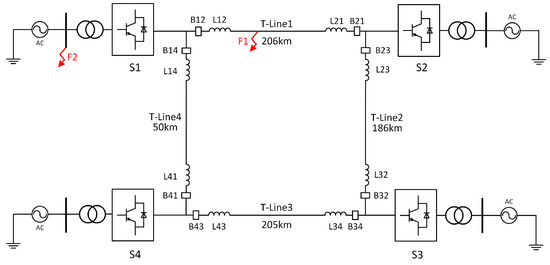
Figure 1.
Netted four terminal MMC-MTDC transmission system.

Table 1.
Simulation parameters of the test model.
3. Pole-To-Ground Fault Analysis
The main damage of pole-to-ground fault is that the healthy pole voltage would rise to twice the rated value. Meanwhile, the AC side voltage has a large DC bias and the transformer may not be able to withstand this [25]. This represents a great challenge for line insulation and transformer operation. Due to the adoption of small current grounding methods, the fault current of the pole-to-ground fault is smaller than that of the pole-to-pole short circuit fault. The primary advantage is that any overcurrent wouldn’t damage power devices and extraordinary protection is not required on bridge arms, however, it also causes difficulty for detecting the fault. In fact, as long as there is no tripping of the converter stations, the control operation can be maintained and active power can be exchanged as scheduled [26]. In a MMC-MTDC transmission system based on overhead transmission lines, fault currents generally include several different components and the characteristics under different grounding methods are completely different [24].
3.1. Grounding Scheme
At present, there are three main grounding schemes:
- Through star-connected reactors and a large resistor at AC side.
- Adopting a resistor at the neutral point of AC side transformer (delta/star configuration).
- Using two large resistors in parallel at the DC side.
The specific structures are shown in Figure 2. In the first grounding scheme, the large reactor Lg and R are used to limit the fault current rising speed and steady-state value, respectively. Depending on the DC voltage level, the resistance ranges from several hundred to more than one thousand Ohms. The second grounding scheme is usually used in low voltage system, it characterized by using the transformer secondary side star winding instead of the star-connected reactors to save grounding equipment and its grounding resistance is large, too. The fault characteristics on the DC side of the two grounding schemes are similar, however, a large fault current could flow through the transformer secondary side using the second scheme during a pole-to-ground fault, which would increase the difficulties of transformer manufacture.
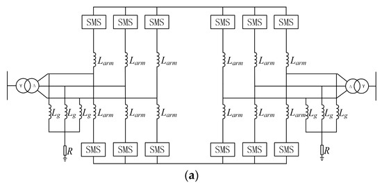
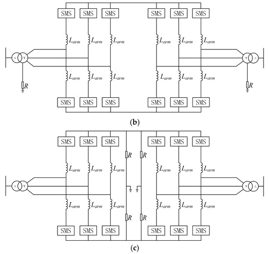
Figure 2.
Specific structure of the MMC grounding scheme. (a) Through star-connected reactors and a large resistor at AC side; (b) Adopting a resistor at the neutral point of AC side transformer; (c) Using two large resistors in parallel at the DC side.
The third grounding scheme would cause additional losses and the two serial DC resistors would probably lead to a voltage imbalance between the positive pole and negative pole due to a certain amount of resistance deviation. In high-voltage and large-capacity MMC-MTDC systems, using the latter two ground scheme would amplify their shortcomings and the grounding point on the transformer converter-side could provide a zero-sequence current path [27], so only the first scheme is suitable for MMC-MTDC. Actually, this scheme is widely used in many practical projects, such as the Trans Bay Cable Project in America. Therefore, this paper only analyzes the first grounding scheme, and the other two methods are not discussed further below.
3.2. Single-Terminal MMC Fault Current Circuit
Each current path of the fault current after positive pole-to-ground fault in a single-terminal MMC is shown in Figure 3.
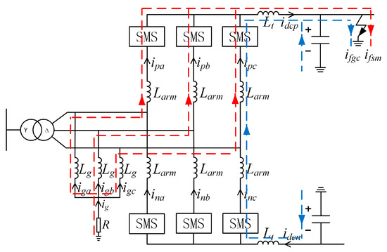
Figure 3.
Fault current circuit in single-terminal MMC when positive pole-to-ground fault.
Their formation reasons are summarized as follows:
- The fault pole arm capacitance would form a discharge circuit through the fault grounding point and the AC side grounding electrode [28].
- The mutated voltage causes the capacitance to earth discharge both in fault and healthy DC line [25].
- Because of the isolation of the transformer, the AC power wouldn’t be connected to fault point, so AC current can remain normal value.
In general, DC fault line current if consists of normal operating current iL, fault pole arm sub-module capacitors discharge current ifsm and capacitance to earth discharge current ifgc, as shown in (1). While only ifsm and ifgc can flow into the fault point. The negative pole-to-ground fault isn’t discussed in detail since it is similar to positive fault:
The simulation waveform of if is shown in Figure 4. There are three components in if as mentioned above. The slowly rising DC component (blue line) corresponds to ifsm because it is in an over-damping circuit, while the high frequency oscillation component represents ifgc, which in an under-damping discharge circuit.
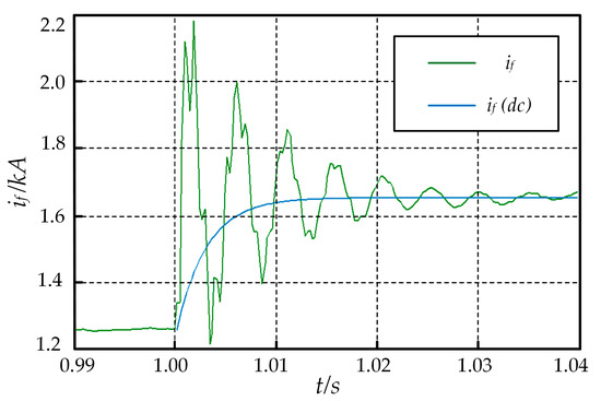
Figure 4.
Schematic diagram of if.
Due to the mutation of DC line voltage, ifgc would rise rapidly within a few microseconds. The above analysis shows that the transient fault current includes ifgc and ifsm in a short time after fault, while the fault steady-state current includes only ifsm. The specific analysis is as follows.
3.3. Sub-Module Discharge Current ifsm
Considering that ifgc would affect the voltage distribution in the fault arm, the equation for the entire circuit of ifsm cannot be established. In order to eliminate the influence of ifgc and to reflect the changing trend of ifsm, the grounding electrode circuit is selected which can be regarded as a first-order circuit with a step voltage source after a pole-to-ground fault. The AC side voltage amplitude can be set as Us before fault and it would radically change −1/2Udc after fault. The following conditions that are obtained according to the circuit parameters are:
Through the three factor method, the ifsm theoretical value can be expressed as:
This expression is verified in MATLAB and the result is shown in Figure 5. The capacitance parameter used in the theoretical value calculation process is 0.0081 μF/km, while line resistance and inductance are ignored. The simulation value is obtained by filtering out iL and ifgc from if. However, the voltages across current limiting reactor and arm reactor are not considered in the simplified model expressed by Equation (3), which makes the difference between the theoretical and simulation value of ifsm.
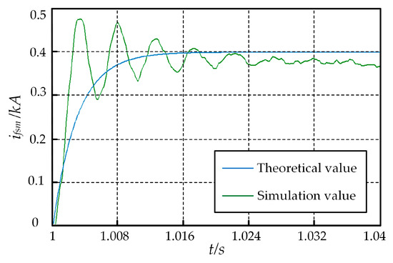
Figure 5.
Theoretical value and simulation value of ifsm.
Since the voltage across current limiting reactor and arm reactor is ignored in the simplified model (3), the simulation value of ifsm in Figure 5 has a fluctuation in the first 20 ms after a fault. The steady-state value of the simulation is smaller than the theoretical value, which is caused by the sub-module capacitor voltage reduction. Like simplified model (3) can still reflect the changing trend and rising value of ifsm to a certain extent. Similar to AC single-phase grounding faults and two-phase short circuit grounding faults, DC pole-to-ground faults also belong to a kind of unsymmetrical fault. This would make the DC positive current different from the negative current and the difference is ifsm. The relationship can be expressed as:
The grounding electrode current ig is usually 0 during normal operation, while it increases significantly after a fault due to the inflow of ifsm. This is a feature compared with the pole-to-pole fault, which can be seen as a sign of pole-to-ground faults.
3.4. Transmission Lines Discharge Current ifgc
After a DC pole-to-ground fault, both the positive and negative DC line would produce ifgc. The fault current direction is shown in Figure 6.
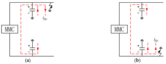
Figure 6.
Fault current circuit of ifgc. (a) Positive pole-to-ground fault; (b) Negative pole-to-ground fault.
When a positive fault occurs, the positive line voltage rapidly reduces to 0 and the line capacitance would discharge to earth, while the absolute value of the negative line voltage increases at the same time, so its line capacitance to earth would be charged. It can be seen that the discharge current and charge current both flow from the earth to the transmission lines, so the two currents are in the same direction. Similarly, after a negative pole-to-ground fault, the ifgc of positive line and negative line are both flowing from the transmission lines to the earth. Therefore, whether a positive or negative fault, the ifgc of positive and negative lines are superimposed on each other, which is different from a pole-to-pole short circuit fault.
Because the ifgc produced by fault pole directly flows to the fault point, the protection device at the end of the fault line can only detect the fault current ifgc of a healthy pole. Considering the voltage change of every element in the circuit, the healthy pole capacitance on the earth discharge circuit can be simply equivalent to a second order RLC circuit as shown in Figure 7.
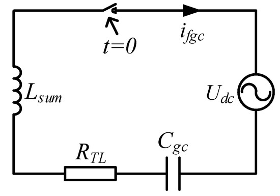
Figure 7.
ifgc equivalent circuit.
Lsum represents a two series arm inductance. RTL represents line resistance. Cgc is the negative line capacitance on earth. Since Cgc is usually much smaller than the sub-module capacitance, it can represent the equivalent capacitance value of the whole circuit. When t = 0, the switch closes and the voltage source starts to charge Cgc. The initial condition is:
We establish the loop equation according to KVL:
Substituting the initial condition into (2), it can be approximated as:
The simulation and theoretical values obtained through MATLAB are shown in Figure 8. The variation trends of the two curves are basically the same, but the amplitude and transient are slightly different. Because the control system would change the original switching order of sub-modules and complicate the fault current transient process the MMC control system is a non-linear and time variable system, which is difficult to model with a mathematical model. Considering the parameters of general overhead lines, the oscillation frequency of ifgc is about hundreds of Hertz. That is to say, ifgc can reach a large value in about 1 ms after a pole-to-ground fault. This feature can be used for grounding fault protection of MMC transmission lines.
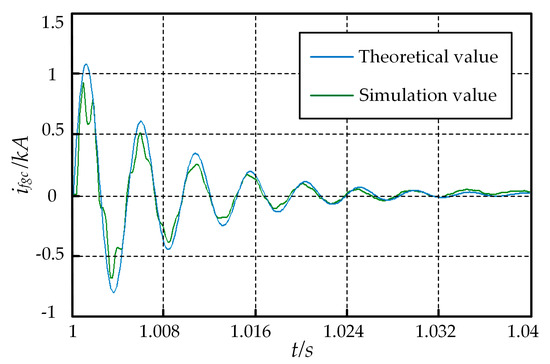
Figure 8.
Theoretical value and simulation value of ifgc.
3.5. Multi-Terminal MMC Fault Current Circuit
The fault current distribution of multi-terminal MMC system is more complex than that of single-terminal MMC. For a two-terminal MMC shown in Figure 9, there exists another current i’fsm after a fault shown as the red dotted line. The capacitance of lower arms in both converters is connected to the fault discharge circuit, but due to the symmetry of the two converter stations, there is also a similar fault circuit that flows from the left converter grounding electrode to the fault point. Although the magnitude of i’fsm is different in each phase and varies with time, the sum of three phases can be seen as a fixed value. When the converter station parameters are identical, the i’fsm generated by the two converters can be canceled out by each other. Therefore, in general, i’fsm has little effect on transmission lines.
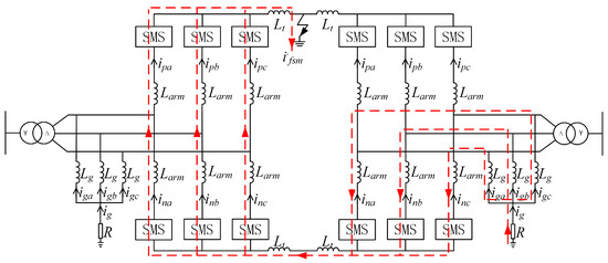
Figure 9.
Fault current circuit in double-terminal MMC during positive pole-to-ground fault.
Assuming that the phases of the two AC systems are close, the lower arm voltage in each phase of the two converters is offset, so it can be surmised that only the sub-modules in the upper arm are discharged after a pole-to-ground fault. With the development of a fault, the upper arm sub-module capacitor voltage drops obviously. The control system is bound to increase the AC current to compensate for the energy loss. If no additional arm energy balance control method is adopted, this will lead to a voltage rise in the lower arm capacitance [20]. Finally, the energy imbalance of upper and lower arms results in system collapse.
In conclusion, only the upper arm sub-modules are discharged in converters during a positive pole-to-ground fault, and the discharge current includes two parts: ifsm through the grounding electrode in local converter and i’fsm through grounding electrodes in other converters. And the two parts of the current are in parallel. The ifgc produced by the capacitance to earth would reach the first peak in about 2 ms and oscillates in tens of milliseconds. The fault steady state current is determined by ifsm.
4. Protection Scheme
The fault rate of long distance overhead lines is high and it seriously threats the normal operation of the DC power grid. MMC-MTDC needs to use ultra-high-speed protection to detect and locate the fault line to protect other parts of the grid [22]. At present, the traditional DC protection methods are too slow and may cause damage to the power devices. For this reason, a fast protection scheme is proposed for pole-to-ground fault detection and location in MMC-MTDC based on the transient characteristics described in Section 3.
Using the communication-based protection method can detect and locate the fault more accurately, but in long distance transmission lines, the protection delay caused by communication would increase the fault expansion. The communication device itself may also have a certain failure rate. So the protection method proposed in this paper uses only local information for fault detection.
The protection scheme is described based on the system shown in Figure 1. When fault F1 occurs, protection B12 and B21 at the two ends of fault line TLine1 should ensure quickly detection of the fault and tripping DC circuit breakers. At the same time, other protections at healthy lines should not operate. The proposed protection scheme is as follows.
4.1. Protection Start-up Unit
The start-up unit can detect a fault or a disturbance to start-up the following fault distinguishing algorithm. At present, the start-up methods usually utilize DC voltage or current amplitude and change rate as starting criteria. An improved voltage gradient method is used for protection start-up since a system abnormality can be characterized by a DC voltage change [29]. The criteria and calculation expression of the protection start-up unit are:
where ∇u(k) is the calculated DC voltage gradient. u(k − i) is the ith sampling voltage value prior to the present moment. Δ1 is the threshold value of the start-up criteria, which should be greater than the normal operating maximum value of ∇u(k). The first sampling point satisfying the criteria is denoted by Ks, and this moment is the protection start time. The sampling step and frequency in this paper are set as 0.05 ms and 20 kHz, respectively. The threshold Δ1 can be set as 0.1 p.u. of the DC voltage as reference. The change rate of DC voltage is quit high after a fault so the threshold Δ1 is nearly instantaneously reached within 0.3 ms.
The improved gradient algorithm is not only simple and convenient, but also makes full use of the high-speed sampling data, which effectively improves the sensitivity of fault detection and has some smooth noise reduction function to meet the requirement of fast protection of DC power grids.
4.2. Determination of the Fault Type and Faulty Poles
As can be known from the transient characteristics of pole-to-ground faults, the increase of grounding electrode current ig is an obvious feature. It rises ten times or even dozens of times after a pole-to-ground fault while it is nearly 0 during normal operation and other fault types. When the protection device detects the suddenly increase of ig, it can be judged that a pole-to-ground fault has occurred in the system. Figure 10 shows the simulation waveform of ig measured in the four-terminal converter stations after fault F1. In normal operation, the maximum of ig is no more than 5 A, but it rapidly reaches 40 A at about 1 ms after a fault.
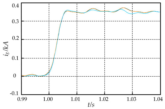
Figure 10.
ig in four stations when positive pole-to-ground fault.
Using an average value can eliminate the error caused by the wrong sampling point and improve the reliability of the protection. The average of ig sampling values in 1 ms is selected as the sign of measurement in this paper:
where is the average value of N continuous sampling points. Ks is determined by Equation (8). Considering the quickness requirement, the protection data window is selected as 0.15 ms and the number of sampling points N is 3.
When negative pole-to-ground fault occurs, ig is negative, as shown in Figure 11. This feature can be used to set the fault type criterion as:
where Δ2 is the current threshold. When ig exceeds the threshold value, the protection can determine whether a positive or a negative pole-to-ground fault has occurred in the grid. With the parameters in Table 1, selecting 100 A as the threshold Δ2 is enough to avoid protection misoperation. In simulation result, the criteria (9) and (10) are satisfied at 2.3 ms after a fault.
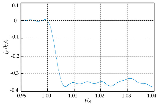
Figure 11.
ig in S1 when negative pole-to-ground fault.
4.3. Fault Location Discrimination
In a multi-terminal MMC grid, it is necessary to determine whether the fault location is in the protection scope or not, which can be seen as fault location. Protection B12 should perform a reliable action after fault F1 yet B41 should remain restrained.
In order to analyze this clearly, intercept converter station S1 and the line connected with it after fault F1 are shown in Figure 12. The blue and red dotted lines represent ifgc produced by a positive line and negative line, respectively. Both the fault line and the health line would produce a large scale ifgc current flowing to the fault point. Considering the distribution parameter characteristics of transmission lines, the amplitude of ifgc flowing through B12, which is closer to the fault point, is larger than that of B41 and ifsm would only add to this trend. Through this point the protection can determine whether or not it should act. The components of a fault current passing through B12 and B41 are respectively recorded as i12 and i41, and the simulation waveforms are shown in Figure 13.
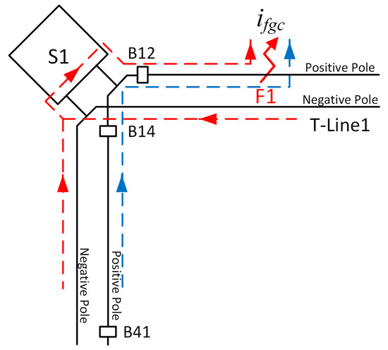
Figure 12.
Distribution of ifgc in S1.
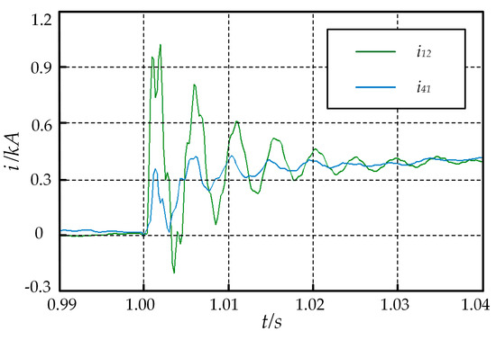
Figure 13.
i12 and i41 when positive pole-to-ground fault.
Since the fault current of a pole-to-ground fault is much smaller than that of a pole-to-pole fault, setting the protection criterion by the amplitude of fault current may result in a decrease in protection sensitivity. Combined with the previous analysis, the fault transient characteristics show that there is a great change of ifgc in about 2 ms after a fault. For this reason, the change rate of the fault current can be selected as the protection criterion. In order to reduce the calculation work, the current change rate can be represented by the current limiting reactor voltage VL [30]. The fault location criterion and calculation formula is:
where ∇VL is the minimum value in N continuous sampling points. Δ3 is the voltage threshold, which is set in accordance with the maximum value of VL when a fault occurs out of the protected area. The protection data window is also selected as 0.15 ms and the number of sampling points N is 3.
The conditions of VL12 and VL41 are shown in Figure 14. Both of them are close to 0 in normal operation, but they differ by several-fold after a fault. That is enough to set a reasonable threshold.
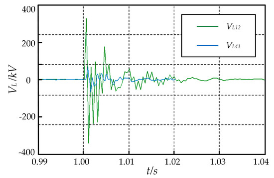
Figure 14.
VL12 and VL41 when positive pole-to-ground fault.
The flow chart of the protection scheme is shown in Figure 15.
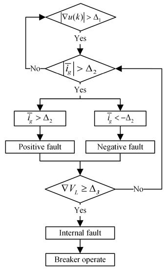
Figure 15.
Proposed protection scheme.
5. Simulation, Sensitivity and Selective Analysis
In order to verify the proposed protection scheme, full-scale simulations have been performed. The simulation model is constructed according to the structure shown in Figure 1 and the parameters in Table 1.
5.1. Protection Threshold Setting and Sensitivity Analysis of Internal Fault
The protection threshold needs to be set reasonably to ensure the protection selectivity and sensitivity. In particular, the value of Δ3 faces complex selectivity requirements due to the different length of transmission lines and the volatile control modes of converter stations in the grid. Based on a large number of simulations for the four-terminal network, the value of VL12 when the pole-to-ground fault occurs at different positions on every positive line is shown in Figure 16.
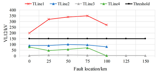
Figure 16.
VL12 value when a positive pole-to-ground fault occurs.
As can be seen from the figure, the value of VL12 varies at different fault locations after a positive pole-to-ground fault occurs in TLine1. The maximum of VL12 is nearly 350 kV and the minimum value is about 200 kV. However, when the fault occurs at other lines, the value of VL12 is no more than 100 kV. Therefore, the Δ3 of protection B12 can be set as 150 kV. Once the value of three continuous sampling points of VL12 are all more than 150 kV, protection B12 can determine that the fault occurs on TLine1, and cut off the fault line through the DC circuit breaker.
When other line protection devices in the grid are chosen as the research object, the simulation results are similar to the curves shown in Figure 16. Only the required simulation results are listed in Table 2 due to the limit of the paper length. Since VL12 is the two order derivative of the fault current, its change rate is quite fast, too. The criterion (11) can be reached in 0.4 ms after a fault, so generally speaking, the satisfying time of criterion (10) determines the fault detection speed and fault F1 can be detected and located within 3 ms in theory.
Table 2.
Extreme value of VL detected by line protection devices and protection threshold Δ3.
In Table 2, Vfmin represents the minimum value of the current limiting reactor voltage when it is on the fault line. Vhmax indicates the maximum value of the current limiting reactor voltage when it is on the healthy line. According to the selectivity and sensitivity of protection, Δ3 can be appropriately set between Vfmin and Vhmax. In this paper, a series of reference Δ3 values are given as a demonstration, while many other factors such as fault resistance would still need to be considered in actual projects.
5.2. Protection Performance and Sensitivity Analysis of External Fault
The protection scheme proposed in this paper is suitable for the rapid detection of pole-to-ground faults occurring on DC transmission lines, so the faults on the AC side and pole-to-pole faults on DC lines are external faults. The performance of the protection scheme after external faults is analyzed below.
When a fault occurs on the AC side, the protection of each line in the grid should not act. The simulation of a three-phase short circuit fault on S1 AC bus is made as example. The simulation waveforms of VL12 and VL41 are shown in Figure 17. Neither of the voltage reaches the protection threshold after a fault, and so do other protections in the grid. Therefore, the protection scheme is not affected by AC side faults.
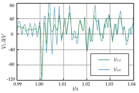
Figure 17.
VL12 and VL41 during AC side faults.
When a pole-to-pole short circuit fault occurs on DC transmission lines, the sub-modules of upper and lower arms are discharged rapidly. The fault current on the DC line rises sharply, and the value of VL is much larger than that of the pole-to-ground fault. However, similarly to an AC three-phase short circuit fault, DC pole-to-pole faults are symmetrical faults. The current flowing through the positive and negative lines after a fault are equal and there is no fault current flowing into the ground electrode, so the value of ig is still close to 0. Even though the fault location criterion may be satisfied, the value of ig would not exceed the protection threshold, so the protection will not malfunction. Figure 18 shows the simulation results where ig is basically unchanged in the case of a DC pole-to-pole fault.
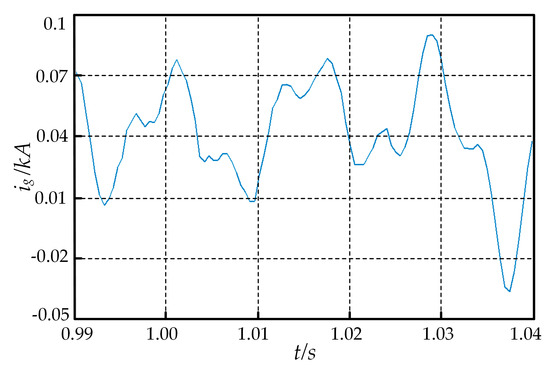
Figure 18.
ig during DC pole-to-pole fault.
5.3. Fault Resistance
The impact of fault resistance is not taken into account in the foregoing discussion. However, the existence of fault resistance may affect the fault detection and location. It limits the fault current to a certain extent and the value of VL may not able to reach the protection threshold, which leads to a decrease of protection sensitivity. Still taking protection B12 as the object, the specific analysis of fault resistance influence is presented.
Normally, the fault resistance of a DC overhead line fault is not more than 100 Ω. Three typical resistance conditions are considered in this paper: 50, 100 and 300 Ω. When a positive pole-to-ground fault occurred in different positions of TLine1 through different fault resistances, the maximum value curve of VL is shown in Figure 19. When the fault resistance and fault distance are both at their maximum value, VL is still greater than the set 150 kV protection threshold. Protection can act exactly, illustrating that the proposed protection scheme has the ability to resist fault resistance.
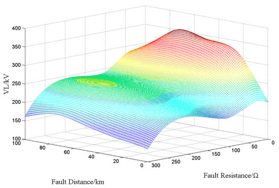
Figure 19.
The maximum value of VL when positive pole-to-ground fault in different positions through different fault resistance.
6. Conclusions
In this paper, the pole-to-ground fault characteristics of MMC-MTDC based on overhead lines are firstly analyzed in detail. A fault transient current mainly includes the fault pole side arm sub-module discharge and transmission line capacitance to earth discharge. According to the fault characteristics, a new high-speed pole-to-ground fault protection scheme based on local information is proposed. The protection data window is short and the action speed is fast. A DC four-terminal network simulation model is built in PSCAD/EMTDC. Through a large number of simulations, it is verified that the proposed protection scheme can accurately detect faults and correctly choose the fault line within 3 ms after a fault. Meanwhile, the scheme meets the requirements of protection selectivity and sensitivity, and has the ability to withstand fault resistance to a certain extent.
Acknowledgments
The work presented was funded by The National Key Research and Development Program (No. 2016YFB0900901), The National Natural Science Foundation of China (No. 51577129) and The Natural Science Foundation of Tianjin (No. 14JCYBJC21000).
Author Contributions
Shimin Xue and Jie Lian put forward the idea and theoretical verification. Shimin Xue conceived and designed the simulation model. Jie Lian performed the simulation and drafted the article. Jinlong Qi and Boyang Fan analyzed the data. All four were involved in revising the paper.
Conflicts of Interest
The authors declare no conflict of interest.
References
- Lesnicar, A.; Marquardt, R. A new modular voltage source inverter topology. In Proceedings of the 10th European Conference on Power Electronics and Application, Toulouse, France, 2–4 September 2003. [Google Scholar]
- Lesnicar, A.; Marquardt, R. An innovative modular multilevel converter topology suitable for a wide power range. In Proceedings of the IEEE Bologna Power Tech Conference, Bologna, Italy, 23–26 June 2003. [Google Scholar]
- Oates, C. Modular multilevel converter design for VSC HVDC applications. IEEE J. Emerg. Sel. Top. Power Electron. 2015, 3, 505–515. [Google Scholar] [CrossRef]
- Marquardt, R.; Lesnicar, A. New concept for high voltage-modular multilevel converter. In Proceedings of the IEEE Power Electronic Specialists Conference, Aachen, Germany, 20–26 June 2004. [Google Scholar]
- Dorn, J.; Gambach, H.; Strauss, J.; Westerweller, T. Trans bay cable-a breakthrough of VSC multilevel converters in HVDC transmission. In Proceedings of the CIGRE Colloquium on HVDC and Power Electronic Systems, San Francisco, CA, USA, 7–9 March 2012. [Google Scholar]
- Tang, G.; He, Z.; Pang, H.; Huang, X.; Zhang, X. Basic Topology and Key Devices of the Five-Terminal DC Grid. CSEE J. Power Energy Syst. 2015, 1, 22–35. [Google Scholar] [CrossRef]
- Bresesti, P.; Kling, W.L.; Hendriks, R.L.; Vailati, R. HVDC connection of offshore wind farms to the transmission system. IEEE Trans. Energy Convers. 2007, 22, 37–43. [Google Scholar] [CrossRef]
- Kang, X.; Wang, R.; Ma, X. Parameters Optimization of DC Voltage Droop Control Based on VSC-MTDC. In Proceedings of the IEEE PES Asia-Pacific Power and Energy Engineering Conference (APPEEC), Xi’an, China, 25 October–28 October 2016. [Google Scholar]
- Xue, Y.; Xu, Z. On the Bipolar MMC-HVDC Topology Suitable for Bulk Power Overhead Line Transmission: Configuration, Control, and DC Fault Analysis. IEEE Trans. Power Deliv. 2014, 29, 2420–2429. [Google Scholar] [CrossRef]
- Li, R.; Adam, G.P.; Holliday, D.; Fletcher, J.E.; Williams, B.W. Hybrid Cascaded Modular Multilevel Converter With DC Fault Ride-Through Capability for the HVDC Transmission System. IEEE Trans. Power Deliv. 2015, 30, 1853–1862. [Google Scholar] [CrossRef]
- Yao, L.; Wu, J.; Wang, Z. Pattern analysis of future HVDC grid development. Proc. Chin. Soc. Electr. Eng. 2014, 34, 6007–6020. [Google Scholar] [CrossRef]
- Ademi, S.; Tzelepis, D.; Dysko, A.; Subramanian, S.; Ha, H. Fault current characterisation in VSC-based HVDC systems. In Proceedings of the IET Conference on Development in Power System Protection, Edinburgh, UK, 7–10 March 2016. [Google Scholar]
- Jin, Y.; Fletcher, J.E.; O’Reilly, J. Short-circuit and ground fault analyses and location in VSC-based DC network cables. IEEE Trans. Ind. Electron. 2012, 59, 3827–3837. [Google Scholar] [CrossRef]
- Tang, L.; Ooi, B. Protection of VSC-multi-terminal HVDC against DC faults. In Proceedings of the Power Electronics Specialists Conference, Cairns, Australia, 24–27 June 2002. [Google Scholar]
- Tang, L.; Ooi, B. Locating and isolating DC faults in multi-terminal DC systems. IEEE Trans. Power Deliv. 2007, 22, 1877–1884. [Google Scholar] [CrossRef]
- Wang, S.; Zhou, X.; Tang, G. Analysis of submodule overcurrent caused by DC pole fault in modular multilevel converter HVDC system. Proc. Chin. Soc. Electr. Eng. 2011, 31, 1–7. [Google Scholar] [CrossRef]
- Li, R.; Xu, L.; Holliday, D.; Page, F.; Finney, S.J.; Williams, B.W. Continuous Operation of Radial Multiterminal HVDC Systems Under DC Fault. IEEE Trans. Power Deliv. 2016, 31, 351–361. [Google Scholar] [CrossRef]
- Suo, Z.; Li, G.; Li, R.; Xu, L.; Wang, W.; Chi, Y.; Sun, W. Submodule configuration of HVDC-DC autotransformer considering DC fault. IET Power Electron. 2016, 9, 2776–2785. [Google Scholar] [CrossRef]
- Zhao, C.; Xu, J.; Li, T. DC fault ride-through capability analysis of full-bridge MMC-MTDC systems. Sci. China Ser. E 2013, 43, 106–114. [Google Scholar] [CrossRef]
- Hu, J.; Xu, K.; Lin, L.; Zeng, R. Analysis and Enhanced Control of Hybrid-MMC-based HVDC Systems during Asymmetrical DC Voltage Faults. IEEE Trans. Power Deliv. 2017, 32, 1394–1403. [Google Scholar] [CrossRef]
- Tzelepis, D.; Ademi, S.; Vozikis, D.; Dy´sko, A.; Subramanian, S.; Ha, H. Impact of VSC Converter Topology on Fault Characteristics in HVDC Transmission Systems. In Proceedings of the IET International Conference on Power Electronics Power, Glasgow, UK, 17–19 April 2016. [Google Scholar]
- Kontos, E.; Pinto, R.T.; Bauer, P. Fast DC fault Recovery Technique for H-bridge MMC-based HVDC Networks. In Proceedings of the IEEE Energy Conversion Congress and Exposition, Montreal, QC, Canada, 20–24 September 2015. [Google Scholar]
- Bucher, M.K.; Franck, C.M. Fault Current Interruption in Multiterminal HVDC Networks. IEEE Trans. Power Deliv. 2016, 31, 87–94. [Google Scholar] [CrossRef]
- Yang, G.; Bazargan, M.; Xu, L.; Liang, W. DC Fault Analysis of MMC Based HVDC System for Large Offshore Wind Farm Integation. In Proceedings of the IET Renewable Power Generation Conference, Beijing, China, 9–11 September 2013. [Google Scholar]
- Bi, T.; Wang, S.; Jia, K. Short-Term Energy Based Approach for Monopolar Grounding Line Identification in MMC-MTDC System. Power Syst. Technol. 2016, 40, 689–695. [Google Scholar] [CrossRef]
- Kontos, E.; Bauer, P. Analytical Model of MMC-based Multi-terminal HVDC grid for Normal and DC Fault Operation. In Proceedings of the IEEE Power Electronics and Motion Control Conference, Hefei, China, 22–25 May 2016. [Google Scholar]
- Li, R.; Fletcher, J.; Xu, L.; Williams, B. Enhanced Flat-Topped Modulation for MMC Control in HVDC Transmission Systems. IEEE Trans. Power Deliv. 2017, 32, 152–161. [Google Scholar] [CrossRef]
- Zhao, C.; Li, T.; Yu, L. DC Pole-to-ground Fault Characteristic Analysis and Converter Fault Recovery Strategy of MMC-HVDC. Proc. Chin. Soc. Electr. Eng. 2014, 34, 3519–3526. [Google Scholar] [CrossRef]
- Kong, F.; Hao, Z.; Zhang, S.; Zhang, B. Development of a Novel Protection Device for Bipolar HVDC Transmission Lines. IEEE Trans. Power Deliv. 2014, 29, 2270–2278. [Google Scholar] [CrossRef]
- Li, R.; Xu, L.; Yao, L. DC Fault Detection and Location in Meshed Multi-terminal HVDC System Based on DC Reactor Voltage Change Rate. IEEE Trans. Power Deliv. 2017, 32, 1516–1526. [Google Scholar] [CrossRef]
© 2017 by the authors. Licensee MDPI, Basel, Switzerland. This article is an open access article distributed under the terms and conditions of the Creative Commons Attribution (CC BY) license (http://creativecommons.org/licenses/by/4.0/).