Influence of Soundtrack on Eye Movements During Video Exploration

Abstract

Models of visual attention rely on visual features such as orientation, intensity or motion to predict which regions of complex scenes attract the gaze of observers. So far, sound has never been considered as a possible feature that might influence eye movements. Here, we evaluate the impact of non-spatial sound on the eye movements of observers watching videos. We recorded eye movements of 40 participants watching assorted videos with and without their related soundtracks. We found that sound impacts on eye position, fixation duration and saccade amplitude. The effect of sound is not constant across time but becomes significant around one second after the beginning of video shots.

Introduction

Over the past hundred years attention - the focus on one aspect of an environment while ignoring others - has become one of the most intensely studied topics within cognitive neurosciences. Different studies tried to determine which part of signals captured by different senses (e.g. vision, hearing, touch) generates attention. In this field of research, most studies have been dedicated to visual attention. Since 1980, numerous visual attention models have been proposed (Tsotsos et al., 1995; Itti, Koch, & Niebur, 1998; Le Meur, Le Callet, & Barba, 2007). These models break a visual signal down into several feature maps dedicated to specific visual features (orientation, spatial frequencies, intensity, etc.). In each map, the spatial locations that locally differ from their surroundings are emphasized. Then, maps are merged into a master saliency map, which points out regions that are the most likely to attract the visual attention of observers.

Studies in cognitive neurosciences have established a close link between visual attention and eye movements. The premotor theory of spatial attention posits that visual attention and oculomotor system share the same neural substrate (Rizzolatti, Riggio, Dascola, & Umilta´, 1987). This theory has been strengthened by recent neurophysiological experiments which have shown that intracranial subthreshold stimulation of several oculomotor brain areas results in enhanced visual sensitivity at the corresponding retinotopic location (Belopolsky & Theeuwes, 2009). Although some other studies suggest a greater separation of the two processes (Klein, 1980), the existence of a high correlation between eye movements and visual attention meets general consensus.

This link between visual attention and eye movements allows authors to evaluate their visual attention models by comparing the predicted salient regions with the locations actually looked at by observers during an oculometric experiment (Parkhurst, Law, & Niebur, 2002; Itti, 2005; Le Meur et al., 2007). These models were initially built for static images, but since motion plays a very important role in visual attention (Yantis & Jonides, 1984), they rapidly evolved to be used with videos (Carmi & Itti, 2006; Marat, Ho-Phuoc, et al., 2009).

All the cited models are bottom-up (i.e. based on stimulus properties), and hence are particularly suitable for dynamic stimuli: the constant appearance of new salient regions promotes bottom-up influences at the expense of top-down strategies (i.e. induced by the subject), making models more stable over time. Indeed, the high consistency of eye movements when watching dynamic scenes both within and across observers is a characteristic that is often outlined in the literature (Goldstein, Woods, & Peli, 2007; Hasson et al., 2008; Dorr, Martinetz, Gegenfurtner, & Barth, 2010). Aside from motion, other features such as faces or top-down influences have been integrated into visual attention models (Torralba, Oliva, & Castelhano, 2006; Marat, Guyader, & Pellerin, 2009). However, these features always belong to visual modality. When using eye tracking and dynamic stimuli, authors do not mention the soundtracks or explicitly remove them, making participants look at ”silent movies” which is far from natural situations. Up to now, the influence of sound on eye movements has been left aside.

Nevertheless, clues for the existence of audio-visual interactions in attention are numerous. Audio-visual illusions are certainly the most popular ones. For example the McGurk effect, where mismatched acoustic and visual stimuli result in a perceptual shift : auditory /ba/ and visual /ga/ are audio-visually perceived as /da/ (McGurk & MacDonald, 1976). Another well-known audio-visual interaction is the help given by ”lip reading” to understanding speech, even more when speech is produced in poor acoustical conditions or in a foreign language (Jeffers & Barley, 1971; Gailey, 1987; Summerfield, 1987). Studies have shown that when presenting audio-visual monologues, perceivers gazed more at the mouth as auditory masking noise levels increased (Vatikiotis-Bateson, Eigsti, & Yano, 1998).

Besides these perceptual phenomena, some studies have tried to develop models of cross-modal integration. To this end, influences of competing visual and auditory stimuli on different behavioural measurement and on the shifts of gazes have been examined. Authors showed that speed and accuracy of eye movements in detection tasks were improved when using a congruent audio-visual stimulus compared to a mere visual or auditory stimulus (Corneil & Munoz, 1996; McDonald, Teder-Sa¨leja¨rvi, & Hillyard, 2000; Corneil, Van Wanrooij, Munoz, & Van Opstal, 2002; Arndt & Colonius, 2003). In their study, Quigley, Onat, Harding, Cooke and Konig (2008) presented static natural images and spatially localized (left, right, up, down) simple sounds. They compared eye movements of observers when viewing visual only, auditory only or audio-visual stimuli. Results indicated that eye movements were spatially biased towards the regions of the scene corresponding to the sound sources.

However, spatial localization is not necessary to observe the influence of sound on visual attention. One study (Burg, Olivers, Bronkhorst, & Theeuwes, 2008) stated that a nonspatial auditory signal improved spatial visual search. The correct mean reaction time was up to 4 seconds shorter (depending on the number of distractors) when a nonspatial beep was synchronized with the visual target change. After controlling alternative explanations of the so-called pip and pop phenomenon (an auditory ”pip” makes the visual target pop out), the authors proposed that the temporal information of the auditory signal directly interacted with the synchronous visual event. As a result, the visual target became more salient within its environment.

Nonspatial auditory information has also been used with visual saliency to generate video summaries (Rapantzikos, Evangelopoulos, Maragos, & Avrithis, 2007; Evangelopoulos et al., 2009). In these studies, authors computed and coupled visual and auditory saliencies to detect the most salient frames, chosen to make up the video summary.

Apart from one preliminary study discussed below (Song, Pellerin, & Granjon, 2011), the influence of non-spatialized sound on eye movements made by observers watching videos has never been explored. To investigate that issue, we checked if eye movements of observers changed when looking at videos with their original soundtracks and without any sound. We compared the regions fixated in the scenes as well as eye movement parameters such as saccade amplitude and fixation duration.

Methods

Participants

Participants were made up of 40 undergraduate and PhD students from the University of Grenoble (France): 26 men and 14 women, ages ranging from 20 to 29 years (M = 25.3, SD = 2.7). Participants were not aware of the purpose of the experiment and gave their consent to participate. This study was approved by the local ethics committee. All were French native speakers, had a normal or corrected to normal vision and reported normal hearing.

Apparatus

Participants were seated 57 cm away from a 21 inch CRT monitor with a spatial resolution of 1024 x 768 pixels and a refresh rate of 75 Hz. The head was stabilized with a chin rest, forehead rest and headband. The audio signal was presented via headphones (HD280 Pro, 64Ω, Sennheiser). Participants wore headphones during the whole experiment, even when the stimuli were presented without soundtrack. Eye movements were recorded using an eyetracker (Eyelink 1000, SR Research) with a sampling rate of 1000 Hz and a nominal spatial resolution of 0.01 degree of visual angle. Thus, an eye position was recorded every millisecond in binocular ”pupil - corneal reflect” tracking mode. Each experiment was preceded by a calibration procedure, during which participants focused their gaze on 9 separate targets in a 3 x 3 grid that occupied the entire display. A drift correction was carried out between each video, and a new calibration was done at the middle of the experiment and if the drift error was above 0.5˚.

Stimuli

We chose 50 video sequences with their original soundtracks. When the soundtrack contained speech, it was always in French. Several studies showed that eye movements are impacted by movie editing style (Dorr et al., 2010). Here, we chose only extracts from professional movies (action movies, drama, documentary films, dialogues). Each video sequence has a resolution of 720 x 576 pixels (30 ˚ x 24 ˚ of visual angle) and a frame rate of 25 frames per second. They last from 0.9 s to 35 s (M = 8.7 s; SD = 7.2 s). As a whole, video sequences last 23.1 min. As explained in the introduction, we chose to focus on the influence of nonspatial sound on eye movements, hence, we used monophonic stimuli. For the cases (41 out of 50 videos) where the original audio signal was stereo, we added the two channels and sent the result to both headphones.

Most of the video sequences we used were made of several shots, separated from each other by shot cuts. A shot cut is an abrupt transition from one shot to another that greatly impacts visual exploration (Garsoffky, Huff, & Schwan, 2007; Smith, Levin, & Cutting, 2012). Thus, we did not study whole videos but we analyzed each shot. Shots were automatically detected using the pixel by pixel correlation value between two adjacent video frames. We ensured that the shot cuts detected were visually correct. Sequences contained different number of shots, with a total number of 163 shots. In the analyzes, we separated the first shot of each video (50 shots) from the others (113 shots) because the central fixation cross preceding each video biased gazes at the beginning of the first shot.

Procedure

The experiment was designed using a software named SoftEye (Ionescu, Guyader, & Gue´rin-Dugue´, 2009). It is a flexible software that allows the stimulus presentation to be synchronized with the eyetracker. It releases, in a single file, all the required data for further analysis: eye positions, events (saccades, fixations and blinks) detected by the Eyelink system, stimulus beginning and ending. Figure 1 illustrates the time course of experimental trials. Before each video sequence, a fixation cross was displayed in the center of the screen for 1 second. After that time, and only if the participant looked at the center of the screen (gaze contingent display), the video sequence was played on a mean grey level background. Between two consecutive video sequences a grey screen was displayed for 1 second.

Participants had to look freely at 50 videos. In order to avoid any order effect, videos were randomly displayed. Twenty participants saw the first half of videos in the visual condition (i.e. without any sound) and the other half in the audio-visual condition (i.e. with their original soundtracks), with a small break in between. Stimulus conditions (Visual and Audio-Visual) were counterbalanced between participants. Finally, each video sequence was seen in the visual condition by 20 participants and in the audio-visual condition by 20 other participants.

Analysis

Data

We discarded data from four subjects due to recording problems.

Eye positions per frame We only analyzed the guiding eye of each subject. The eye tracker system gives one eye position each millisecond, but since the frame rate is 25 frames per second, 40 eye positions per frame and per participant were recorded. In the following, an eye position is the median position that corresponds to the coordinates of the 40 raw eye positions recorded per frame and per subject. Frames containing a saccade or a blink were discarded from eye position analysis. For each frame and each stimulus condition, we discarded outliers, i.e. eye positions above ±2 standard deviations from the mean.

Saccades, fixations and blinks Besides the eye positions, the eye tracker software organizes the recorded movements into events: saccades, fixations and blinks. Saccades are automatically detected by the Eyelink software using three thresholds: velocity (30 degrees/s), acceleration (8000 degrees/s2) and saccadic motion (0.15˚ ). Fixations are detected as long as the pupil is visible and as long as there is no saccade in progress. Blinks are detected as saccades with a partial or total occlusion of the pupil. We did not use them in this analysis. For each stimulus condition, we discarded outliers, i.e. saccades (resp. fixations) whose amplitude (resp. duration) was above ±2 standard deviations from the mean.

We separated the recorded eye movements into two sets of data. First, the data recorded in the audio-visual (AV) condition, i.e. when videos were seen with their original soundtrack. Then, the data recorded in the visual (V) condition, i.e. when videos were seen without sound.

Metrics

Dispersion To estimate the variability of eye positions between observers, we used a measure called dispersion. For a frame and for n participants (thus n eye positions p = (x_i, y_i)i∈[1..n]), the dispersion D is defined as follows:

In other words, the dispersion is the mean of the Euclidian distances between the eye positions of different observers for a given frame. If all participants look at the same location, the dispersion value is small. On the contrary, if eye positions are scattered, the dispersion value increases. Note that this metric has some limitations: there might be more than one region of interest, and thus, eye position cluster around these regions. Hence, the dispersion would increase even though eye positions are located in the same few region of interest. In this analysis, we computed a dispersion value for each frame of the 163 shots. First, we took the mean dispersion over all frames (global analysis). Then, we looked at the frame by frame evolution of dispersion (temporal analysis). For both analyses, we compared the dispersion within conditions (intra V and AV dispersions) and the dispersion between stimulus conditions (inter dispersion). If soundtrack impacts on eye position dispersion, we should find a significant difference between the mean intra AV and V dispersions.

Distance to center The distance to center is defined as the distance between the barycenter of a set of eye positions and the center of the screen. This distance reflects the central bias, and we analyzed its evolution along shots. The central bias expresses the fact that when exploring visual scenes, the gaze of observers is often biased toward the center of the screen. In this analysis, we computed a distance to center value for each frame of the 163 shots in each stimulus condition.

KL-divergence The Kullback-Leibler divergence is used to estimate the difference between two probability distributions. This metric can be compared as a weighted correlation measure between two probability density functions. It was already used to compare distributions of eye positions (Tatler, Baddeley, & Gilchrist, 2005; Le Meur et al., 2007; Quigley, Onat, Harding, Cooke, & K¨onig, 2008). The KL-divergence (KLD) between two distributions Q^a and Q^b is defined as follows, with p the size of the distributions:

The lower the KL-divergence is, the closer the two distributions are.

In this analysis, we computed, for each frame of the 163 shots, two density maps (one for each condition): QV and QAV. For a given frame, a 2D Gaussian patch (one degree wide) was added to each eye position. These maps are the same size as video frames (p = 720 x 576 pixels) and are normalized to a 2D probability density function. Then, we computed the KL-divergence between QV and QAV (inter KL-divergence): the lower the KL-divergence is, the closer the two maps are, and the more the participants in V and AV conditions tend to look at the same positions.

First, we took the mean KL-divergence over all frames (global analysis). Then, we looked at the frame by frame evolution of KL-divergence (temporal analysis). For each analysis, we compared the inter KL-divergence with the KL-divergence between two maps drawn from two random sets of eye positions. We also compared the inter KL-divergence with the intra V and AV KL-divergences, defined as the KL-divergence between two maps drawn from the eye positions recorded under the same stimulus condition. These maps were created by randomly splitting each dataset of 20 participants in two subgroups of 10 participants. We repeated this random split 10 times and took the mean KL-divergence. If soundtrack impacts on eye position locations, we should find a significant difference between the mean inter and intra KL-divergences. Dispersion and KL-divergence are two complementary metrics. Dispersion provides information about the variability between eye positions, but does not tell anything about the relative position of the two data sets of eye positions for the two stimulus conditions. For the KL-divergence, it is the opposite.

Results

The aim of this research is to quantify the influence of soundtrack on eye movements when freely exploring videos. To this end, we compared the eye movements recorded on video sequences seen in visual (V) and audio-visual (AV) conditions, using different metrics. First, we analyzed the eye positions of participants (dispersion and Kullback-Leibler divergence). Then, we focused on two eye movement parameters: saccade amplitude and fixation duration.

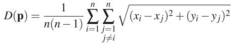
Inter V-AV Intra AV Intra V Figure 2. Mean dispersion values: between all eye positions (blue), between eye positions recorded in audio-visual condition (green) and between eye positions recorded in visual condition (red). Dispersions are given in visual angle (degrees) with error bars corresponding to standard errors.

Figure 2. Mean dispersion values: between all eye positions (blue), between eye positions recorded in audio-visual condition (green) and between eye positions recorded in visual condition (red). Dispersions are given in visual angle (degrees) with error bars corresponding to standard errors.

Figure 2. Mean dispersion values: between all eye positions (blue), between eye positions recorded in audio-visual condition (green) and between eye positions recorded in visual condition (red). Dispersions are given in visual angle (degrees) with error bars corresponding to standard errors.

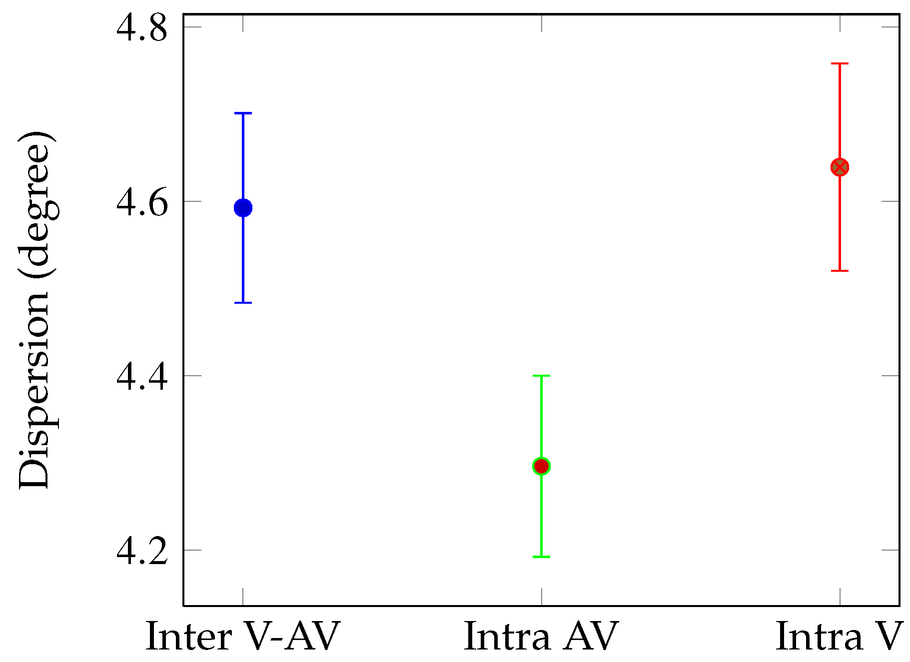
Figure 3. Mean Kullback-Leibler divergence between the eye position distributions in the V and AV conditions (blue), between two sets of eye positions extracted from the AV (green) and the V (red) conditions. Error bars correspond to standard errors.

Figure 3. Mean Kullback-Leibler divergence between the eye position distributions in the V and AV conditions (blue), between two sets of eye positions extracted from the AV (green) and the V (red) conditions. Error bars correspond to standard errors.

Eye position variability (dispersion)

Global analysis We compared the mean dispersion for all the 163 shots according to three conditions (see Figure 2): Intra AV (green bar), Intra V (red bar) and Inter (blue bar). We performed t-test on the mean dispersions for 163 observations (video shots). The dispersion is lower for the AV condition than for the V (t(324)=2.17, p < 0.03) and the Inter V-AV condition (t(324)=1.97, p < 0.05). This result means that on average, there was less variability between the eye positions of observers when they explored videos with their original soundtracks.

We also performed a mixed-factor ANOVA, with the stimulus condition (V and AV) the within-subjects factor and stimulus condition order (AV-V and V-AV) the between-subjects factor. It revealed that the stimulus condition order had no effect.

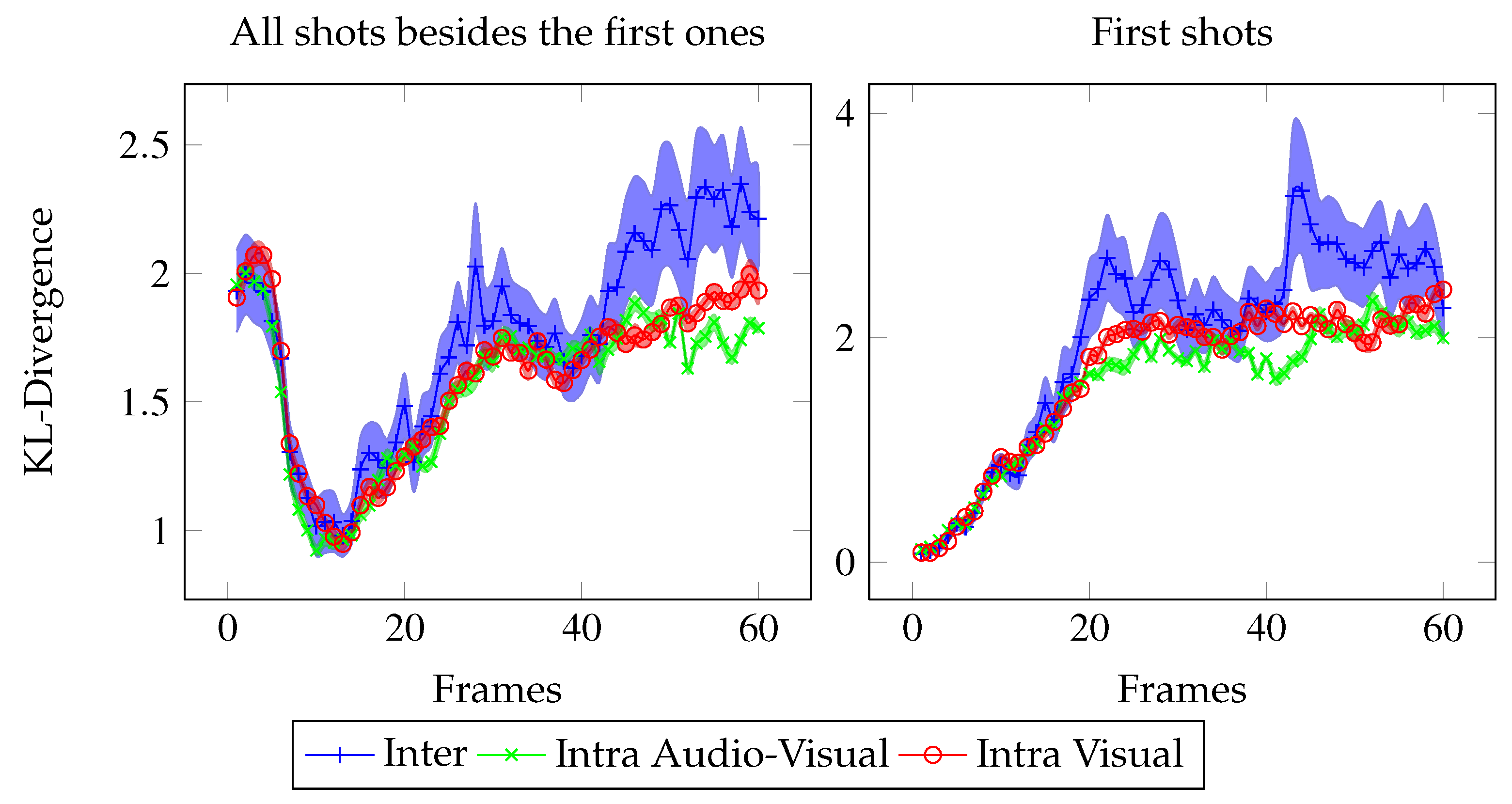
Temporal analysis Since we worked on dynamic stimuli, it is interesting to analyze the temporal evolution of the dispersion along shots to see how the influence of sound evolves along video shots exploration. On the left side of Figure 4, the temporal evolution of the dispersion and of the distance to center are plotted, averaged over all the shots except the first ones, i.e. the shots that were not impacted by the central cross before video onset.

During the first 3 frames after a shot cut, the dispersion (resp. the distance to center) is stable. During this period, the gaze of observers stays at the same locations as before the cut. Then, from frame 4 to 10, the dispersion and the distance to center dip deeply. From frames 11 to 25, curves both increase regularly. This leads to the last stage where the dispersion (resp. the distance to center) fluctuates around a mean stationary value.

The temporal evolution of the dispersion and of the distance to center averaged over all the first shots are slightly different (see the right side of Figure 4). Before each video, participants were asked to look at a fixation cross in the center of the screen. Hence, during the 3 first frames, both the dispersion and the distance to center are low in both AV and V conditions (as previously, gazes stay at the same locations as before the cut, i.e. at the center of the screen). Then, curves increase linearly and reach a plateau, which was identical to previously in the left-hand plots, except that the mean value is here slightly higher.

The following statistics are performed on all 163 shots. Until the 25th frame (∼1 s), no clear distinction can be made between V and AV conditions: the red and green curves overlay each other. However, after that (i.e. when the curves have stabilized) the mean value of dispersion in V condition is significantly above the one in AV condition (t-test: from frame 1 to 25 : t(324)=1.85, n.s.; from frame 25 to end : t(324)=2.06, p < 0.05).

For the distance to center, the opposite occurs: during the stabilized phase, the AV condition curve is mostly above the V condition curve. Nevertheless, this relation is not statistically significant. Note that the separation before vs. after frame 25 is not a clean-cut classification, but is estimated from the shapes of the dispersion and distance to center curves.

To sum up, around one second after shot onset, participants in AV condition are less dispersed than participants in V condition. Moreover, participants in AV condition tend to look away from the screen center more than participants in V condition. These results will be further discussed.

Eye position locations (KL-divergence)

Global analysis We compared the mean KL-divergence for all the 163 shots according to 3 conditions (see Figure 3): Intra AV (green bar), Intra V (red bar) and Inter (blue bar). The random KL-divergence (M = 6.13) is high above the others and is not plotted. We performed t-test on the mean KL-divergences for 163 observations (video shots). The KL-divergence is higher for the Inter condition than for the Intra AV (t-test: t(324)=2.27, p < 0.05) and V conditions (t(324)=1.69, p < 0.05). This result means that on average, sound impacts the fixated locations. The congruency between fixation locations is higher inside respective both conditions than between the two different stimulus conditions.

Temporal analysis Figure 5 presents the frame by frame Inter KL-divergence (in blue), Intra V KL-divergence (in red), and Intra AV KL-divergence (in green). The KL-divergence temporal evolution follows the same pattern as the dispersion: during the first 25 frames, no distinction can be made between intra and Inter KL-divergences. However then, the Inter KL-divergence is significantly above the Intra AV and V KL-divergences (respective t-test: from frame 1 to 25, t(324)=1.55, n.s. and t(324)=1.21, n.s.; from frame 25 to end, t(324)=2.1, p < 0.05 and t(324)=1.94, p < 0.05).

Fixations and saccades

We analyzed the distributions of fixation duration and saccade amplitude made by participants in V and AV conditions. In both stimulus conditions, both parameters follow a positively skewed, long-tailed distribution, which is classical when studying such parameters during scene exploration (Bahill, Adler, & Stark, 1975; Pelz & Canosa, 2001; Tatler, Baddeley, & Vincent, 2006; Tatler & Vincent, 2008; Ho-Phuoc, Guyader, Landragin, & Gue´rin-Dugue´, 2012).

We performed paired t-test on median saccades amplitude and median fixation duration for 36 observations (participants). We observed shorter saccade amplitudes in V condition (Mdn = 3.01 ˚ ) than in AV condition (Mdn = 3.17 ˚ ; t(35)=2.35, p < 0.05). Shorter fixation durations in V condition (Mdn = 290 ms) than in AV condition (Mdn = 298 ms) were observed, but this difference is only a tendency (t(35)=1.6, p = 0.1).

Discussion

We compared eye positions and movements of participants looking freely at videos with their original soundtracks (AV condition) and without sound (V condition). We found that the soundtrack of a video influences the eye movements of observers. Since we found that the influence of sound is not constant over time, it is crucial to understand the temporal evolution of eye positions on dynamic stimuli, regardless of the stimulus condition. Hence, before discussing the impact of sound on eye movements, we first focus on the dynamic of eye movements during video exploration.

Eye movements during video viewing

In our experiment, we chose to use dynamic stimuli - and more precisely professional movies - for the following reasons. Eye movements made while watching videos are known to be highly consistent. It is true both between different observers watching the same video and between repeated viewing of the same video by one observer (Goldstein et al., 2007). Nonetheless, this consistency depends on the movie content, editing and directing style (Hasson et al., 2008; Dorr et al., 2010). Indeed, authors found much more correlation between the recorded eye movements and brain activity during professional movies than during amateur ones. 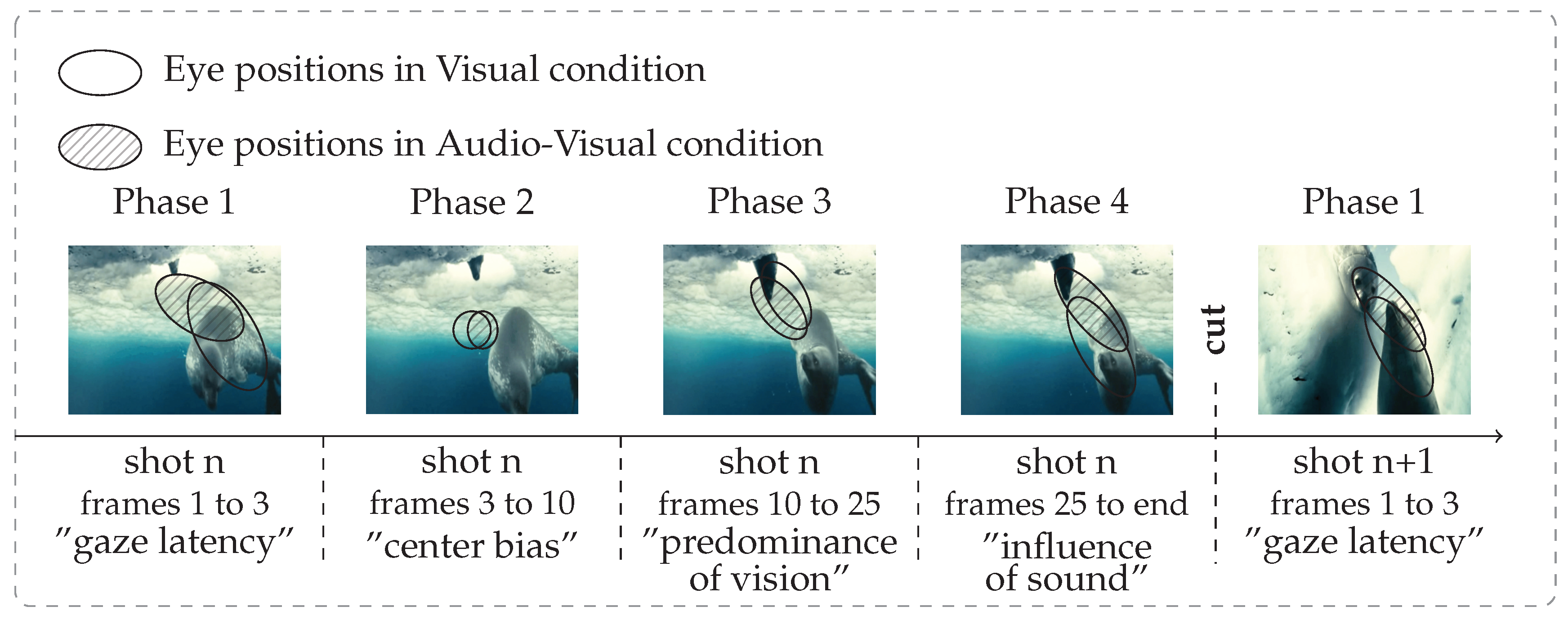It reflects that in a general way, eye movements are strongly constrained by the dynamics of the stimuli (Boccignone & Ferraro, 2004). In particular, video shot cuts have a great impact on gaze shift (Boccignone, Chianese, Moscato, & Picariello, 2005; Mital, Smith, Hill, & Henderson, 2010). A shot cut is an abrupt transition from one scene to another, and eye movements depend more on this transition than on contextual information (Wang, Freeman, Merriam, Hasson, & Heeger, 2012). Thus, in this study, we analyzed eye movements over shots rather than over the all videos. We found that after each cut, the eye position variability (dispersion), the mean distance between eye positions and the center of the screen (distance to center) and the difference between eye position locations (KL-divergence) followed the same pattern. Independently of stimulus condition, we identified four phases during video exploration, summarized in Figure 6. Our time unit is a video shot.

Phase 1: from frame 1 to 3 (∼120 ms) after shot onset, gazes remain at the last position they were in on the previous shot. Dispersion, distance to center and KL-divergence are stable. Phase 1 stands for the latency needed by participants to start moving their eyes to a new visual scene. This delay is classically reported for reflexive saccades toward peripheral target (latency around 120-200 ms (Carpenter, 1988)).

Phase 2: from frame 4 to 10 (∼240 ms), gazes go to the center of the screen (which is the optimal position for a rough overview of the scene), dispersion, distance to center and KL-divergence drop sharply. This behaviour is known as the center bias, see (Tatler, 2007; Tseng, Carmi, Cameron, Munoz, & Itti, 2009; Dorr et al., 2010).

Phase 3: from frame 11 to 25 (∼500 ms), dispersion, distance to center and KL-divergence increase regularly. This phase is classical in scene exploration literature: bottom-up influences are high and participants begin to explore the scene in a consistent way (Tatler et al., 2005). This behaviour is indicated by a rising distance to center (after getting closer to the center of the screen, gazes begin to move away) and by a still low dispersion and KL-divergence. Nevertheless, top-down (i.e. subject specific) strategies rise, inducing a gradual increase of dispersion between participants.

Phase 4: from frame 25 to the end, dispersion, distance to center and KL-divergence oscillate around a stationary value. In dynamic stimuli, the constant appearance of new salient regions promotes bottom-up influences at the expense of top-down strategies. This induces a stable consistency between participants over time (Carmi & Itti, 2006; Marat, Ho-Phuoc, et al., 2009).

Influence of sound across time

Psychophysical studies showed that synchronized multimodal stimuli lead to faster and more accurate responses during target detection tasks, e.g. (Spence & Driver, 1997; Corneil et al., 2002; Arndt & Colonius, 2003). Other studies trying to address this issue are often based on the spatial bias induced on eye movements by sound sources. Often, authors modulate the visual saliency map with the sound source position map (Quigley et al., 2008; Ruesch et al., 2008). Our approach is different: we studied the effect of nonspatial (monophonic) sound on the eye movements of observers viewing videos. Indeed, we hypothesized that sound might be extracted to form a new feature which interacts with visual saliency, bringing about a change in the gaze of the observers.

In a preliminary study, we elicited the effect of video editing (shots and cuts) by averaging dispersion between eye positions on all the frames of videos made up of several shots, and found no significant evidence for an effect of sound on eye movements (Coutrot, Ionescu, Guyader, & Rivet, 2011). The new study presented in this paper points out the importance of considering the video editing impact on the temporal course of eye movements, as mentioned in the previous paragraph.

Through the first three phases, sound does not have a significant effect on eye positions: we found that the dispersion in V and AV conditions overlap, as well as the inter and intra KL-divergences. This shows that during the beginning of scene exploration, the influence of sound is outweighed by visual information. During the last phase, the dispersion is lower and the distance to center higher in AV condition than in V condition. Furthermore, inter KL-divergence is higher than intra KL-divergences, which shows that fixation locations are different between the two conditions. This behaviour might be explained if we consider that sound strengthens visual saliency: without sound, participants’ gaze might be less attracted to salient regions. This hypothesis is confirmed by the difference in saccade amplitude distributions: participants in AV condition make larger saccades than participants in V condition. This is coherent with the idea that participants in AV condition move their gaze further away from the center of the screen. Moreover, participants in AV condition tend to make longer fixations than participants in V condition. According to our hypothesis, salient regions might attract participants’ gaze for a longer time period in AV condition. These results are consistent with a recent study that investigated the oculomotor scanning behavior during the pip and pop experiment (Zou, Mu¨ ller, & Shi, 2012). The authors found that spatially uninformative sound events increase fixation durations upon their occurrence and reduce the mean number of saccades. More specifically, spatially uninformative sounds facilitated the orientation of ocular scanning away from already scanned display regions not containing a target. It is interesting to observe that these results are the same whether the stimuli are complex and natural (the videos we used) or very simple (bars and auditory pip). Note that in a preliminary study, sound induced a tendency to increase dispersion (Song et al., 2011), but this effect was not statistically tested.

These results indicate that models predicting eye movements on videos could significantly be improved by considering non spatial sound information. In their study, Wang, Freeman, Merriam, Hasson, and Heeger (2012) proposed a simple model for eye movements during video exploration: at the beginning of each shot, the observers seek, find and track an interesting object, each cut resetting the process. The model provided a good fit to experimental eye position variance. Here, we show that to be complete this model should consider two more stages: gaze persistence at the last location of the previous shot three frames after a cut and gaze centering before the exploration of salient regions (phases 1 and 2). Moreover, the parameters of the model should be different depending on the presence or absence of sound. For instance, the probability of finding a point of interest following a saccade should be higher with than without sound.

Conclusion

In this study, we showed that during video exploration, gaze is impacted by the related soundtrack, even without spatial auditory information. We showed that in audio-visual condition, the eye positions of participants are less dispersed and tend to go more away from the screen center, with larger saccades. Moreover, we showed that observers do not look at the same locations when videos are seen with or without sound. Our results highlighted that the effect of sound is not constant across time: we did not find any significant effect of sound after abrupt visual changes (shot cuts). All these results indicate that adding sound as a new feature to classical visual saliency models might improve their efficiency. The next step would be to determine the most efficient way to insert this new attribute into visual saliency models. In particular, one would test the influence of a specific sound on specific visual features. For instance, one can assume that sound does not impact faces the same way as landscapes.