Abstract
This study examines how physical and transition climate risks affect the greenium, assuming that implied volatility serves as a proxy for investor sentiment generated by these risks. Applying a Gated Recurrent Unit (GRU) deep learning model to daily data from January 2020 to June 2025 with a rigorous train–test split to get around the drawbacks of full-sample estimations and guarantee strong out-of-sample generalizability is a significant empirical contribution. Our findings show that adding the interaction between these climate risks and the sentiment proxy slightly increases predictive power. The GRU model outperforms random forest and linear regression benchmarks in terms of generalizability, but it remains sensitive to different data splits and hyperparameter tuning. This highlights the use of complex, non-linear models for risk forecasting and portfolio allocation for investors and risk managers, as well as the need for regular climate disclosure for policymakers to reduce information asymmetry. The GRU’s stringent validation framework directly enables more reliable pricing and exposure management.
1. Introduction
Understanding how financial markets respond to climate-related threats has become a crucial area of contemporary research. The adequate way of incorporating the economic implications of physical and transition risks stemming from climate change into asset valuations by the investor represents the concept of climate pricing risk (Eren et al., 2022). Investors start to become interested in the implications of risk disclosure on financial stability, including physical and transition climate risks. Transition risks arise from the ongoing shift toward a low-carbon economy. They encompass the potential impacts of mitigation and adaptation policies, the development of cleaner technologies, and the evolving behaviours of consumers and investors. In contrast, physical risks result from changes in the climate itself, namely, long-term alterations in average temperatures, weather variability, and the frequency or intensity of extreme climatic events (Campiglio et al., 2023).
The rising demand for investment strategies that incorporate environmental, social, and governance factors has significantly increased investor interest in sustainable financial products. In this context, green bonds and green equities constitute the two primary categories of environmentally oriented investment instruments (Ferrer et al., 2021). These instruments are often structured around green indices, which are replicated through Exchange-Traded Funds (ETFs), generally considered less risky than traditional funds (Yue et al., 2020). In this study, we focus on green bonds as they continue to attract interest from institutional investors prioritising sustainability goals. However, pursuing more ambitious green investment targets does not necessarily lead to larger green bond allocations. The outcome largely depends on investors’ risk aversion, highlighting the complex interplay between risk preferences and goal-oriented utility in shaping green investment decisions (Chen et al., 2025). According to (Löffler et al., 2021) Green bonds generally yield approximately 15–20 basis points lower returns than comparable conventional bonds in both primary and secondary markets, suggesting that investors are willing to accept a lower yield in exchange for holding environmentally sustainable assets. In (Dorfleitner et al., 2022) The investors tend to reward green bonds that have undergone external verification, as such reviews confirm the bonds’ genuine environmental purpose and prior market access (Fatica et al., 2021). These verified green bonds are typically associated with a premium, reflected in lower yields and a higher price, commonly referred to as the greenium, representing the yield differential between conventional and green bonds and can be expressed as:
Hence, risk disclosure emerges as a key factor influencing investors’ decisions, as it signals the credibility and authenticity of the green bond. However, it remains uncertain whether these green ETFs consistently outperform their conventional, non-green counterparts (Heldmann et al., 2025), even with the risk disclosure present. Vestrelli et al. (2024) argue that climate risk disclosures are generally associated with higher firm value. However, this relationship may weaken or even become negative when attention to climate change intensifies. This can be explained by the lower yields on green bonds, which allow firms to raise funds more cheaply, reflecting investors’ preference for sustainability. Nevertheless, heightened attention to climate risks can increase yields, lowering the value of green bonds and potentially reducing firm value. These dynamics suggest that the green bond market is influenced by investor sentiment, where perceptions and preferences regarding sustainability and climate risk affect bond yields and firm value beyond what can be justified by fundamentals. According to (W. Wang, 2024) Such sentiment-driven behaviour introduces stochastic elements into trading, making asset prices less predictable and reducing the scope for effective arbitrage. This sentiment component can, in turn, generate a risk-off environment, as investors become more risk-averse and demand higher yields to compensate for the perceived increase in risk (Johar et al., 2022). Extending the findings of (Dragotto et al., 2025), who demonstrates that market sentiment significantly influences the greenium, this study posits that risk disclosure acts as a key driver of investor sentiment, and incorporating a proxy for market sentiment into the analysis is essential to capture the influence of sentiment on pricing dynamics and market stability.
In sum, it can be inferred that the relationship between the greenium, risk disclosure, and market sentiment is inherently complex and cannot be adequately captured by simple models. Such dynamics are particularly relevant for transition risk, where regulatory uncertainty and concerns about greenwashing may lead to divergent investor behaviours (Y. Zhang et al., 2025). Similarly, under physical risk, factors such as heightened media attention and the occurrence of climate-related disasters can amplify investor reactions and market volatility. Also, from a behavioural finance perspective, investors are not always fully rational, and information asymmetries, often reinforced by these events, can distort price formation, causing asset prices to deviate from fundamental values and allowing some investors to earn abnormal profits, thereby emphasising the significant role of market sentiment (Andleeb & Hassan, 2023). The intricate interplay between investor perception, sustainability preferences, and disclosure dynamics requires a more advanced methodological approach. In this regard, deep learning models emerge as a suitable and powerful tool to uncover this complexity and provide deeper insights into the underlying mechanisms driving green bond pricing and investor behaviour. A non-linear temporal model using direct indicators of physical and transition risk is therefore suited to capture the sentiment-driven behaviour of the greenium.
In this context, green bonds fulfil a dual role, catering both to investors’ traditional financial objectives and their environmental goals. Consequently, green impact investors may derive utility not only from financial returns but also from the positive environmental outcomes associated with their investments. Within this extended utility framework, which goes beyond the behavioural finance perspective of investor irrationality, green bonds may command higher prices than comparable conventional bonds, as the non-financial utility from environmental impact can compensate for lower financial yields. At the same time, increased attention to climate-related risks can raise yields, potentially reducing green bond values and firm worth. Previous research has attempted to capture these complex dynamics using linear or non-linear models, but a key limitation lies in the reliance on the entire dataset, which restricts the models’ capacity to fully capture complexity and limits the potential for generalisation to unseen data. This represents a research gap. The novelty of the present study lies in its methodological approach: by dividing the data into training and testing sets within a non-linear modelling framework, the study enhances the model’s capacity for generalisation. Furthermore, a robustness analysis comparing the non-linear model with random forecasts and linear regression is conducted to evaluate their relative predictive performance. This approach tests whether the model can accurately predict the greenium using the selected explanatory variables, thereby strengthening the validity and generalizability of the study’s findings.
In their study, Nunes et al. (2025) find that Long Short-Term Memory (LSTM) outperform multilayer perceptrons (MLPs) for medium-term forecasts and reveals regime-switching behaviour and specialisation within LSTM units in daily bond yields. This approach advances explainable artificial intelligence in finance, contrasting with black-box deep learning applications and offering a transparent, dynamic forecasting tool for fixed-income markets. Fischer and Krauss (2018) find that LSTM outperform the random forecast, a deep neural net and logistic regression, attributing success to patterns like short-term reversal and high volatility. LSTM represents a widely used deep learning approach for modelling nonlinear relationships. However, the complex internal architecture of the LSTM can make training challenging (Troiano et al., 2020). To address this, the present study utilises a simplified variant of LSTM, the Gated Recurrent Unit (GRU), which has fewer gates and offers greater flexibility for modelling nonlinear dynamics. Substituting the LSTM with a GRU can yield equal or even superior performance across numerous time series datasets (Elsayed et al., 2019).
This study aims to evaluate the predictive capability of a Gated Recurrent Unit (GRU) model in capturing the nonlinear dynamics of green bond pricing, using key explanatory variables influencing these prices. Specifically, it examines how physical risk indicators (PRI) and transition risk indicators (TRI) affect the greenium over time. These factors can generate a sentiment-driven behaviour among investors, influencing their perceptions and reactions to climate-related risks. To account for this effect, the implied volatility index (VIX) is included as a proxy for market sentiment (Smales, 2017; H. Zhang & Giouvris, 2022), as it reflects investors’ collective perception of risk and uncertainty. Although alternative sentiment indices exist, they are not included in this study.
To what extent can the GRU deep learning model capture the nonlinear relationships through which PRI, TRI, and VIX jointly influence green bond pricing and the greenium, and how does their interaction mitigate fluctuations in green bond yields?
Following the Introduction, the paper transitions to the Literature review, which examines prior research on the existence and determinants of the greenium, highlighting the mixed results and the consistent suggestion that market behaviour is dynamic and nonlinear. The Materials and Methods section then details the empirical approach, including the definition of the daily greenium using the yield spread between the VanEck Green Bond ETF (BGRN) and the iShares Core US Aggregate Bond ETF (AGG). This section outlines the explanatory variables, namely the Physical and Transition Risk Indices, their interaction term, and the VIX as a proxy for market sentiment, alongside the implementation of the GRU model and its training parameters. The Result section presents the statistical characteristics of the greenium and the empirical findings regarding the GRU model’s performance. Finally, the Discussion section interprets these findings, further highlighting their important implications for policy and investment practice.
The study’s contributions are multifaceted, spanning theoretical, empirical, and practical domains. Theoretically, the research advances the literature on climate finance and behavioural asset pricing by integrating Physical Risk Index (PRI), Transition Risk Index (TRI), and the Implied Volatility Index (VIX) into a unified nonlinear framework, which demonstrates how these factors interact to influence greenium dynamics. Empirically, a significant novelty lies in the methodological approach: the introduction of a Gated Recurrent Unit (GRU) deep learning model with data strictly split into training and testing sets. This overcomes a key limitation of prior studies that relied on full-sample estimations, thereby reducing overfitting and substantially improving the model’s out-of-sample validity and generalizability. For policymakers, the findings recommend improving climate disclosure consistency to reduce information asymmetry and mitigate volatility. The link between investor sentiment/volatility and pricing also necessitates coordinated fiscal/regulatory responses during climate-related stress. For investors, the study reveals the greenium as a dynamic, risk-adjusted sentiment premium. This means portfolios should use nonlinear, volatility-aware models for better risk forecasting and asset allocation, helping them exploit temporary mispricing while maintaining sustainable exposure.
2. Literature Review
Prior research has examined the presence of the grenium and its interaction with various determinants. However, the results remain mixed. Some studies report that investors accept lower returns for environmentally sustainable bonds, while others find no significant premium compared to traditional bonds. The Efficient Market Hypothesis posits that asset prices fully and immediately reflect all available information, leaving no room for systematic excess returns (Fama, 1970). In the context of green bond markets, this implies that information related to disclosure factors should already be incorporated into green bond prices and the greenium. Consequently, if prices adjust efficiently, there should be no predictable relationship between these risk indicators and future green bond returns. In a literature survey conducted by (Liaw, 2020), Green bonds are generally found to have lower yields than equivalent conventional bonds, though results vary due to differences in samples, periods, methodologies, and issuer characteristics. Also, green bond funds remain small and typically underperform their benchmarks. Larcker and Watts (2020) and Wurgler (2018) report identical pricing between green and conventional bond issues for the same issuers on the same day, concluding that investors show no particular willingness to pay a premium for green bonds. Nederkoorn and Scholten (2024) report that the greenium is often small or even absent in the primary market, as new bond issues are typically offered at a modest discount to encourage investor uptake. In the secondary market, however, green bonds generally trade at relatively higher prices, reflecting a positive greenium. Nonetheless, prices fluctuate over time, and in some instances, green bonds have been observed to exhibit a slight negative greenium. Accordingly, we hypothesise that green bond prices efficiently incorporate available information, including disclosure factors, such that any observed greenium reflects the market’s pricing of these factors, leaving no predictable patterns in future returns.
Vestrelli et al. (2024) employ a novel text-mining methodology, the Semantic Brand Score (SBS), which leverages social network analysis on quarterly U.S. data from 2020–2022 to quantify climate risk disclosure in 10-K/10-Q reports and climate attention in earnings calls. Using a linear dynamic panel model, they find that climate risk disclosure generally increases firm value. However, a key contribution is their finding that this positive relationship reverses when climate attention is high. Alessi et al. (2021) employ a linear asset pricing model on European stocks (2006–2018), creating a novel greenness and transparency factor from GHG emissions and disclosure quality. It finds a significant negative greenium, meaning investors accept lower returns for greener, more transparent stocks. In a subsequent study, Alessi et al. (2023) extend their earlier work by applying a more sophisticated, time-varying conditional asset pricing model to a larger, unbalanced panel of monthly European stock returns (2006–2020). This updated framework retains the greenness and transparency factor but demonstrates that the greenium is not constant over time; rather, it varies in response to policy developments and market conditions. The study achieves higher explanatory power (R2 values range between 0.88 and 0.94) and provides a more comprehensive empirical framework showing that investor preferences evolve with the perceived credibility of the low-carbon transition. Dorfleitner et al. (2022) analyse 250 matched green-conventional bond triplets with over 90,000 daily observations, using a hybrid regression to estimate a liquidity-adjusted green bond premium. They find a small positive greenium driven mainly by external validations. The R2 values around 0.23–0.34 indicate that their model explains about 23% to 34% of the variation in the green bond premium. The low adjusted R2 values (0.08–0.19) suggest that many of the explanatory variables are not adding much power, which is common in financial studies with noisy data. Dragotto et al. (2025) employ a robust methodology, matching 344 corporate green bonds with conventional counterparts from the same issuer (2014–2022). Its panel regressions, which explain a substantial portion of yield spread variation (R2 = 60–68%), confirm a small but significant average greenium of about −2 basis points. Crucially, the research reveals this premium is highly dynamic, fluctuating with market sentiment and peaking at 16 bps following the Paris Agreement. It extends the literature by demonstrating that third-party certification amplifies the greenium approximately fivefold and that these certified bonds serve as a financial hedge, outperforming conventional bonds during natural disasters and periods of high climate media attention. These findings underscore the critical role of credibility and external validation in sustainable finance.
These results question the core assumptions of Modern Portfolio Theory, which presumes investor rationality, market efficiency, and returns that are exclusively a function of risk. The observed variations in the greenium, shifts in investor preferences, and the influence of third-party certification indicate that non-financial motivations and behavioural elements play a significant role in the pricing of green bonds. This interpretation is consistent with the framework of Behavioural Finance and the “Doing Well by Doing Good” hypothesis expanded in the field of Socially Responsible Investing (SRI), which emerges as a counterpoint to Milton Friedman’s shareholder primacy doctrine. The hypothesis suggests that investors may willingly accept lower financial returns to achieve positive environmental or social outcomes while still maintaining satisfactory overall performance. Empirical and theoretical research consistently demonstrates that such behaviour is inherently nonlinear, even in the absence of deterministic chaos. The empirical study by Inglada-Perez (2020) on major stock indices concludes that while no clear evidence of chaos was found, the markets’ behaviour is unequivocally nonlinear and stochastic. This empirical observation is explained by the theoretical model of Dew-Becker et al. (2025), which shows that such nonlinearities are a near-inevitable outcome of how investors process information. Z. Wang (2025) proposes using deep learning for green bond default risk prediction but lacks methodological specifics, offering no details on model architecture, data sources, sample period, or frequency. It relies heavily on literature review rather than empirical analysis, and while it correctly identifies limitations of traditional linear models and the potential of deep learning, it fails to define variables, sample selection, or training procedures. Without these elements, the proposal remains conceptual and lacks empirical credibility. Y. Zhang et al. (2025) use high-frequency textual data from over 117,000 Chinese earnings calls and broker reports (2013–2023) to construct firm-level climate attention indices. Employing Huber robust regressions within an event-study framework, it finds a significant inverted U-shaped relationship between climate attention and stock returns, particularly for transition risk. This nonlinear finding contrasts with linear-assumption studies and aligns with emerging literature highlighting complex, threshold-based investor behaviour in contexts of high policy uncertainty and information asymmetry, such as China. Therefore, the literature consistently suggests that the greenium is dynamic and investor behaviour is nonlinear, yet most existing analyses rely on linear assumptions; therefore, we hypothesise that the relationship between climate risk disclosure and the green bond premium is inherently complex and dynamic, exhibiting significant time-varying properties that linear frameworks cannot adequately capture. From another standpoint, building on Dragotto et al. (2025) and Johar et al. (2022), market sentiment is considered a key driver of the greenium, and this sentiment is, in part, shaped by risk disclosure. It is proposed that a non-linear temporal model incorporating direct measures of physical and transition risk, along with a proxy for market sentiment, can effectively capture the sentiment-driven dynamics of the greenium. Furthermore, accounting for the broader market sentiment that influences investor behaviour through the inclusion of a general sentiment index is expected to enhance the predictive power of this non-linear framework.
A significant methodological shortcoming in much of the literature concerns the rigour of model validation. Prior studies apply their chosen models, encompassing linear panel regressions, asset pricing models, and nonlinear frameworks, to the entirety of their available dataset without employing a robust train-test split or out-of-sample validation. This approach risks overfitting, where a model appears effective because it describes the specific noise and idiosyncrasies of a single historical sample rather than capturing the true underlying data-generating process. Consequently, the reported explanatory power (e.g., R2) may be inflated, and the identified drivers of the greenium may not be generalizable or reliable for prediction in unseen market conditions.
3. Materials and Methods
3.1. Data Description
This study utilises daily data to capture the dynamics of the green bond market. Daily frequency allows the model to detect rapid changes in the bond pricing that would be smoothed out in weekly or monthly data. The sample period, spanning 6 January 2020 to 30 June 2025, is selected to balance data availability, market representativeness, and the need to include sufficient variability in both financial conditions and risk disclosure variables. By covering this multi-year period, the dataset encompasses different market cycles, extreme events, and variations in attention to climate-related risks, ensuring the model can learn both normal and stressed market dynamics. This choice enhances the robustness and generalizability of the results while providing enough observations for reliable training and testing of the GRU network. We use the VanEck Green Bond ETF (BGRN) as a proxy for green bonds and the iShares Core US Aggregate Bond ETF (AGG) as a benchmark for conventional bonds. Although both ETFs are primarily U.S.-focused, BGRN includes a portion of international bonds1. In contrast, AGG, while classified within the Fixed Income asset class and the Taxable Bond ETF group, allocates approximately 6.2% of its portfolio to foreign issuances2. To capture the differential in yields between green and conventional bonds, we define the daily greenium as the yield spread between BGRN and AGG at time t. Let denote the daily greenium for bonds at time t. It is computed as the difference in daily yield between a conventional bond index and a green bond index ,
where the daily yields are calculated as:
We use the PRI and the TRI from Bua et al. (2024). These indices are based on text-based analysis of Reuters news articles (from January 2005 to the present) using relevance-ranked climate risk vocabularies derived from authoritative scientific texts. Although the index is aggregated and often described as broad-based, its construction is primarily from U.S. sources, including the for example, the Wall Street Journal and the Washington Post…, which means it largely reflects the U.S. financial and policy information environment. Physical and transition risk documents are converted to tf-idf3 vectors, and cosine similarity between daily news and these documents generates a concern series. PRI and TRI are then obtained as AR (1) residuals, reflecting shocks to climate risk discussions. Spikes indicate unexpected increases in attention to physical or transition risks, covering hazards, adaptation and mitigation policies, and net-zero targets. On the other hand, climate risks may interact in complex ways. From another standpoint, firms simultaneously exposed to high TRI and PRI can experience multiplicative effects on bond pricing as the multiplicative terms capture compound extreme events (Laborda et al., 2026). Therefore, including an interaction term between transition and physical risks in the model allows us to capture potential non-linearities arising from their combined impact. Omitting this interaction could lead to biased estimates of the greenium, as the model would fail to account for the joint influence of these climate risk dimensions on bond yields. Moreover, incorporating a proxy of market sentiment can enhance the model’s ability to explain variations in the greenium. In this regard, VIX is identified as the measure of sentiment, as it improves the model fit and provides additional explanatory power.
Now, let’s define the target variable as the values of the and the explanatory variables as . Let the time series dataset be:
where : greenium of the bond at time t, : PRI, : TRI, (: interaction term capturing multiplicative climate effects, and : VIX index, representing market sentiment. Then, the data are arranged into overlapping sequences of fixed length L (lags), where each sequence contains L past observations used to predict the next greenium value:
This formulation enables the model to learn how past information influences future outcomes.
Consequently, the full dataset can be expressed as:
where T represents the total number of available observations. Since neural networks must be trained and evaluated on distinct data portions to avoid overfitting, the constructed dataset is then partitioned into two ordered subsets.
To ensure numerical stability and accelerate convergence, all features are scaled to the interval [0,1] using Min–Max normalisation:
importantly, the scaling parameters are computed only on the training set to prevent data leakage, and then applied to the test set. Then, the data are arranged into overlapping sequences of fixed length L (lags), where each sequence contains L past observations used to predict the next greenium value.
3.2. Empirical Model (GRU)
Once the sequences are prepared, each input is passed through the GRU network to capture nonlinear temporal dependencies. At each time step, the GRU maintains a hidden state that evolves according to the following gating mechanisms. The update gate controls the degree to which the previous memory is retained:
The reset gate determines how much of the past information is forgotten:
Based on these gates, a candidate hidden state is computed as:
Finally, the hidden state is updated as a combination of old and new information:
The hidden state evolves, allowing the model to capture both short-term and long-term dependencies in the greenium dynamics.
Finally, the GRU outputs the predicted greenium:
The GRU parameters , , are optimised by minimising the Root Mean Squared Error (RMSE) between actual and predicted values:
During model training, the root mean squared error (RMSE) (Lewinson, 2020) is commonly used as an optimisation criterion. Many machine learning methods aim to minimise the RMSE when fitting the model to the training data, thereby encouraging the model to generate predictions that are as close as possible to the observed values. RMSE shares the same properties as the mean squared error (MSE); in fact, optimising a model with respect to RMSE yields the same solution as optimising with respect to MSE, since RMSE is simply the square root of MSE (Says, 2023).
Adam optimiser updates the parameters iteratively as:
where η is the learning rate, are bias-corrected first and second moment estimates and a small constant added for numerical stability. In our case, the model is trained over a specified number of epochs with a defined batch size to ensure efficient learning and convergence. Table 1 summarises the key parameters used in the GRU modelling and data processing workflow.

Table 1.
GRU model and data processing parameters.
After training, predictions are generated for both the training and testing samples to evaluate the model’s performance. Performance metrics used in our study are in the Table 2.
Table 2.
Summarises the performance metrics used to evaluate the predictive accuracy of the models.
3.3. Robustness and Sensitivity Analyses
To ensure the robustness and reliability of the model, several complementary analyses were performed. Residuals were examined for white noise behaviour through visual inspections, Q–Q plots, and Ljung–Box tests to confirm the absence of autocorrelation or systematic patterns in model errors. Also, the stability of predictive performance was evaluated by varying the proportion of data allocated to the test set, including 15%, 20%, 25%, and 30% splits. Additionally, the GRU architecture was systematically adjusted, varying hidden layer sizes (32, 64, 128), number of layers (1–3), and dropout rates (0.2–0.4), to assess the impact of hyperparameter choices on model accuracy.
From another angle, the GRU model’s predictions were benchmarked against traditional models, specifically linear regression and random forecast, in terms of training and testing to provide a comparative assessment of explanatory power. Finally, differences between training and testing R2 values were monitored to detect potential overfitting and evaluate the model’s generalisation capacity. This comprehensive approach addresses limitations in previous studies that relied on the full dataset for both linear and non-linear analyses, which constrained generalisation and may have failed to capture complex dynamics. By integrating data splitting, non-linear modelling, interaction terms, and thorough robustness checks, the present study fills a notable research gap and introduces methodological novelty in modelling the greenium.
4. Result
The results indicate promising evidence regarding the significant role of disclosure and market sentiment in explaining the greenium when modelled using the GRU framework. These outcomes highlight the presence of nonlinear and complex interactions between these variables, which traditional linear models may fail to capture effectively.
4.1. Statistical Characteristics of the Greenium
Before proceeding with the analysis, we first begin by examining the statistical characteristics of the greenium (Table 3).
Table 3.
Summary statistics of greenium.
The summary statistics reveal a relatively balanced distribution centred close to zero, with a mean value of −0.000007, suggesting that, on average, the pricing difference between green and conventional bonds is negligible. The standard deviation (0.002237) indicates limited variability, implying that most observations cluster near the mean. However, the range between the minimum (−0.023963) and maximum (0.026419) values shows that, in certain periods or market conditions, the greenium can fluctuate notably in both directions. The interquartile range (from −0.000920 to 0.000866) further confirms that most of the data points lie within a narrow band around zero, suggesting that while the greenium occasionally diverges, such deviations are not typical. This aligns with the findings of Alessi et al. (2023), who report a mixed greenium, and with Nederkoorn and Scholten (2024) and Liaw (2020), who note modest values in the primary market, which can change more significantly in the secondary market. Both TRI and PRI exhibit small negative means with similar dispersion, implying generally mild but variable climate-related shocks. Their interaction term (TRI·PRI) is centred close to zero, consistent with limited but occasionally strong joint effects. The VIX averages around 21, suggesting a moderately volatile market over the sample. The histogram of greenium in Figure 1 illustrates that the distribution is sharply centred around zero, with most observations tightly clustered in a narrow range. This confirms the earlier descriptive statistics indicating a near-zero mean and low standard deviation.
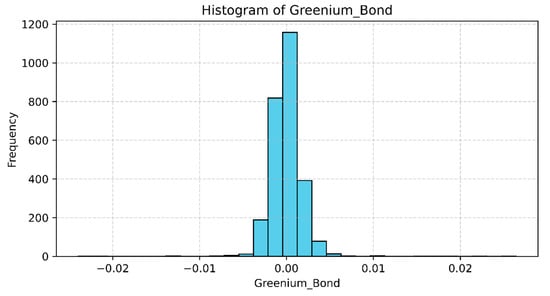
Figure 1.
Histogram illustrating the distributional shape of the greenium.
The histogram of the greenium variable suggests an approximate but not perfect normal distribution. Although it displays a bell-shaped and generally symmetrical form around the centre, it exhibits noticeable deviations from normality. In particular, the distribution appears leptokurtic, with a pronounced peak around zero, indicating that a large proportion of the observations are tightly concentrated near the mean. At the same time, the tails are thinner than expected under a normal distribution, implying that extreme values occur less frequently. This sharp concentration at the centre and the rapid decline in frequency toward the extremes highlight a distribution characterised by high kurtosis and limited dispersion. The Shapiro–Wilk test (Statistic = 0.717242, p-value = 0.000000) confirms that the greenium does not follow a normal distribution, as the p-value is significantly below the 0.05 threshold, leading to the rejection of the null hypothesis. This outcome supports the earlier observation of a leptokurtic distribution, where most values are tightly clustered around the mean with relatively thin tails. In addition, the Augmented Dickey–Fuller (ADF) test (Statistic = −9.281209, p-value = 0.000000) indicates that the greenium series is stationary, meaning it does not contain a unit root. This implies that its statistical properties, such as mean and variance, remain stable over time. Stationarity is a crucial prerequisite for reliable time series modelling, including neural network–based approaches like GRU, ensuring that the model captures genuine dynamics rather than spurious trends. Therefore, it appears well-suited to be analysed using the GRU model in order to explore its potential nonlinear relationships and predictive patterns.
4.2. GRU Model Performance with PRI and TRI
Firstly, we introduce the greenium as the target variable using only PRI and TRI as predictors. Next, we incorporate their interaction effect to capture any combined influence, and finally, we include the VIX to account for broader market volatility in the model. The first output to examine is the loss plot. In our case, it shows promising signs, as there is no indication of overfitting or underfitting, suggesting that the model has a good capacity to generalise to unseen data.
In Figure 2, both the training and testing losses drop very steeply within the first epochs. This indicates that the GRU model is quickly and efficiently learning the underlying patterns of the greenium data. After the initial rapid descent, both loss curves flatten out almost completely, forming a plateau from approximately Epoch 20 to 100. There is no significant change in the loss, indicating the model has converged to its optimal set of weights. Continuing training past 50 epochs offers minimal, if any, performance benefit. The test loss is consistently lower than the training loss throughout the entire training process. This is a highly desirable outcome. It shows that the model generalises exceptionally well to unseen data. There is no evidence of overfitting, which would be indicated by the training loss continuing to decrease significantly while the test loss starts to increase or stays stagnant far above the training loss. The following stage includes the analysis of metrics for both the training and testing sets. Table 4 below presents the corresponding results:
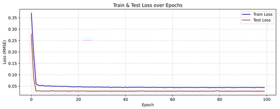
Figure 2.
Training and testing loss of the GRU model incorporating greenium, PRI, and TRI.
Table 4.
Performance metrics of the GRU model on training and testing datasets, using greenium, PRI, and TRI as input features.
The GRU model using PRI and TRI as predictors shows very low R2 values for both the training (0.002851) and testing (0.001382) datasets. This indicates that the model is unable to capture the variance in the greenium, and the predictors alone do not explain the target effectively. These findings suggest that the market is efficient, where the premium already incorporates information from risk disclosure, or that the model is flawed. Then, the use of a linear model captures the essential information, aligning with the prevailing evidence in the literature, which suggests that the underlying relationships are predominantly linear (Alessi et al., 2021, 2023; Dorfleitner et al., 2022; Vestrelli et al., 2024; Dragotto et al., 2025). Although the error metrics (MSE, RMSE, MAE) are numerically small, this is because the greenium values themselves are very close to zero, meaning that even small absolute errors lead to low error values. In addition, both the RAE and the RSE are close to 1, with the RAE slightly exceeding 1 on the testing set, indicating that the model’s prediction errors are generally comparable to a mean-based baseline, though the error is marginally higher for the test data. However, the low R2 further confirms that the GRU model is not learning meaningful patterns from PRI and TRI in this configuration, as observed in the GRU forecast (Figure 3), the predicted line is extremely smooth and remains close to the centre (0.00), whereas the actual series exhibits high-frequency noise and volatility, with spikes reaching up to ±0.02 during the training phase. Similar to the training period, the test predicted line is very smooth and remains flat near 0.00.
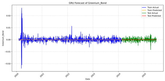
Figure 3.
Predicted values of greenium generated by the GRU model, with PRI and TRI included as predictors.
4.3. Impact of the Interaction Term (PRI∙TRI)
Adding the multiplicative term (PRI∙TRI) has clearly enhanced the predictive power of the GRU model, as shown in the table. While the R2 values are still small, the improvement of R2 to 0.015 for training and 0.022 for testing indicates that nonlinear interactions between PRI and TRI is a slight driver of greenium. Also, the RMSE for both training and testing is improved as the MAE, RAE and RSE (Table 5).
Table 5.
Performance metrics of the GRU model on training and testing datasets after adding (PRI·TRI).
The present findings align with a growing body of literature suggesting that investor reactions to climate disclosures often follow nonlinear patterns (Y. Zhang et al., 2025). Concerning the loss plot (Figure 4), the most notable observation is the overall reduction in loss values compared to the previous model, with the training loss decreasing below 0.05 and the testing loss declining under 0.03, indicating improved model performance.
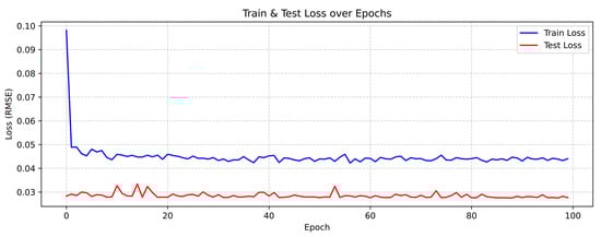
Figure 4.
Evolution of training and testing loss for the GRU model following the inclusion of (PRI·TRI).
This indicates that the engineered multiplicative feature contributes successfully to capturing a complex, non-linear dependency in the data that the GRU was unable to model using the features individually. The updated forecast plot (Figure 5) shows improvement over the previous model:
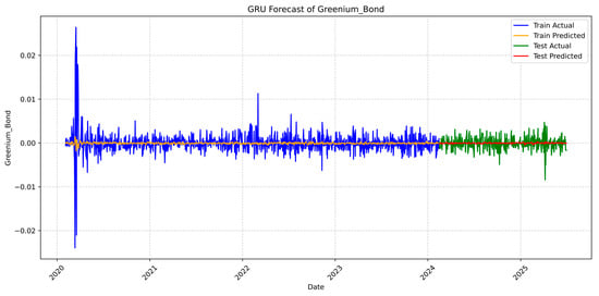
Figure 5.
Forecasted greenium values produced by the GRU model, with (PRI·TRI).
Unlike the previous model, the predicted line now tries to slightly track the short-term spikes and volatility clusters in the actual train set. Similarly, the predicted line in the test period (2024–2025) marginally manages to follow the spikes and dips in the actual test data. This is a critical result for financial forecasting, as it indicates the model is now anticipating periods of high risk. Similar to the findings of Fischer and Krauss (2018) and Nunes et al. (2025), who showed that LSTM models can effectively capture mean-reverting patterns in stock returns, the present results indicate that GRU models exhibit a comparable ability to identify such dynamics in the greenium.
4.4. Incorporating a Proxy for Market Sentiment (VIX)
Adding the VIX index enhances the GRU’s ability to capture variations in the greenium (Table 6). This makes sense intuitively, as VIX reflects market volatility, which can influence the risk premium investors require for green bonds. The combination of PRI, TRI, their interaction, and VIX allows the model to account for both nonlinear effects and market conditions.
Table 6.
Performance metrics of the GRU model on training and testing datasets using VIX as an input feature.
While R2 is still small, it represents an improvement from models without interaction terms or VIX, suggesting that additional macro-financial factors or nonlinear transformations might be needed to capture the remaining variance. This improvement is also evident in the other performance metrics, which show enhanced predictive accuracy. Adding the VIX reduce the loss compared to the simple baseline model (Figure 6), and potentially offers further improvement over the model with just PRI·TRI.
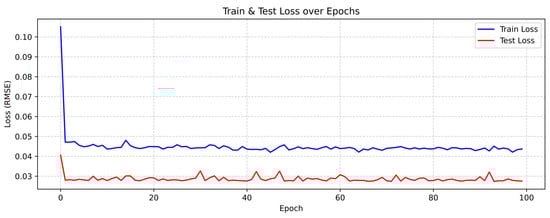
Figure 6.
Evolution of training and testing loss for the GRU model incorporating VIX.
The GRU model’s predicted line is a little more responsive to the extreme spikes and dips in the greenium series (Figure 7), compared to the previous outputs, particularly those associated with market shocks (like the COVID-19 period, where volatility spiked sharply). Volatility spikes are closely linked to market panic and uncertainty.
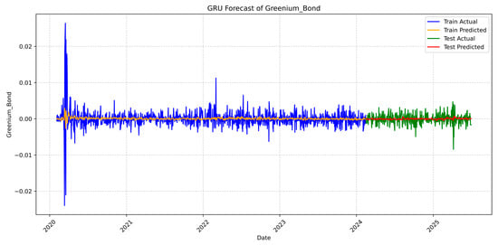
Figure 7.
Forecasted greenium values produced by the GRU model incorporating VIX.
4.5. Evaluation of Model Robustness and Stability
4.5.1. Residual Mean
The unbiased performance of the GRU model is robustly confirmed by the residual mean analysis (Table 7). Both the test mean (−0.000009) and the training mean (−0.000037) are extremely close to zero. This indicates that throughout the whole dataset, the model is not consistently over- or under-predicting the financial variable of greenium. In particular, the near-zero mean on the unseen test data is important because it shows that the model, which takes into account the complex dynamics of market volatility and climate-related risk factors, has learned some of the underlying signal without introducing a generalised systemic bias. This is an important finding for trustworthy financial forecasting and risk assessment.
Table 7.
Residual mean for bias assessment in the GRU model.
4.5.2. Residual Standard Deviation vs. RMSE
The investigation validates the GRU model’s improved resilience and generalisation when applied to the financial risk of greenium. In Table 8, the test residual standard deviation (0.001434) is much lower than the train residual standard deviation (0.002420), indicating that the model performs remarkably well on unseen data. This significant decrease in the prediction error dispersion, which is further supported by the nearly identical RMSE values in the training (0.002421) and testing (0.001434) phases, indicates that the model did not merely memorise training noise, but rather successfully captured the true underlying signal of customer and market dynamics. For predicting greenium’s financial dynamics under complicated, compounded climate-related and market volatility risks, the GRU model is therefore considered to be extremely consistent and reliable.
Table 8.
Comparison of residual standard deviation and RMSE for model performance evaluation.
4.5.3. Shapiro-Wilk Test: The Non-Normality Warning
The Shapiro-Wilk (Table 9) test definitively rejects the null hypothesis of normality for the model errors. The greenium bond histogram, which shows a large central peak and distinct bars in the distant tails, visually confirms this conclusion. This pattern suggests a non-Gaussian, leptokurtic distribution with fat tails, which means that the huge, infrequent prediction errors of the GRU model occur more frequently than would be predicted under a typical Gaussian assumption. This diagnostic is important because it suggests that typical statistical techniques based on normalcy may underestimate the likelihood of extreme financial outcomes for the greenium, even though the model is robust, impartial, and consistent.
Table 9.
Shapiro–Wilk test for normality of residuals in the GRU model.
4.5.4. Visual Diagnostics of Residual Behaviour
The unbiased performance and consistency of the GRU model are strongly confirmed visually by the residuals vs. predicted values plot (Figure 8). The residuals are symmetrically distributed around the zero-horizontal line for both the training and test datasets. The prior statistical conclusion that the residual mean is close to zero, indicating that the model has no systemic bias throughout the range of anticipated values, is supported by this random and centred scatter. Importantly, compared to the training plot, the test plot shows a tighter, more compact grouping of dots, which graphically validates the better generalisation and lower standard deviation on the unknown data. The non-normality finding is supported by the existence of clear, distant outliers, such as the point close to (−0.008) on the test plot, which shows that even though the model is well-specified, high-magnitude prediction errors still happen and need to be taken into consideration in the overall evaluation of greenium’s financial risk.
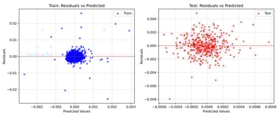
Figure 8.
Residuals vs. predicted values for training and testing sets: homoscedasticity, bias, and outlier analysis.
4.5.5. Residuals over Time: Temporal Dynamics of GRU Model Errors
An essential diagnostic for evaluating the stability of time-series models is the residuals over time display. The model’s stability across the whole sample period is confirmed by the plots (Figure 9) for both the training and test data, which demonstrate that the residuals are stationary, that is, the variance and mean of the errors do not vary systematically over time. The series looks to be steadily centred around zero for the test residuals, indicating the absence of systemic bias. A closer examination of both plots, however, indicates a possible problem: the mistakes seem to show clustering, where tiny errors are followed by little errors and large errors are followed by huge errors. This is particularly evident in the training plot in early 2020 and during the test period. The time-varying structure of the residual volatility suggests that periods of high risk result in periods of less reliable forecasts, a feature frequently encountered in financial time-series modelling, even though the model is generally robust and unbiased.
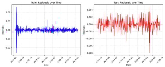
Figure 9.
Residuals over time for training and testing sets: extreme events, stationarity, and volatility clustering.
4.5.6. Residual Distribution and Normality Diagnostics: Fat-Tailed Errors and Robustness Implications
The model’s error characteristics are best illustrated visually via the residuals distribution and Q-Q plots (Figure 10). The model’s impartial performance is further supported by the training and test histograms, which both distinctly display a highly peaked, leptokurtic distribution with heavy concentration around zero. Crucially, there is a clear trend in both the train and test Q-Q plots where the actual points consistently diverge from the predicted straight red line, especially in the upper and lower extremes. With the points rising above the line on the right and falling below the line on the left, this deviation suggests that the residuals have wider tails than a normal distribution. The Shapiro-Wilk test result that the errors are non-normal, which indicates that the GRU model’s prediction errors of large magnitude occur more frequently than standard statistical assumptions would predict, is conclusively confirmed by this visual evidence. This is an important factor for risk assessment under extreme market or climate conditions.
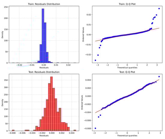
Figure 10.
Residual histograms and Q-Q plots for training and testing sets: visual confirmation of fat-tailed, non-normal errors and extreme event sensitivity.
4.5.7. Ljung–Box Test: Residual Autocorrelation and Implications for GRU Forecasting
The Ljung-Box test is used to determine whether autocorrelation, which defies the presumption that residuals should be independent white noise, is present in the residuals. Table 10 shows that the near-zero p-value for the train residuals indicates that the training residuals are serially correlated and definitively rejects the null hypothesis of no autocorrelation. Though not as strongly as for the training set, the test residuals’ low p-value also results in the null hypothesis being rejected. Although the GRU model is resilient in terms of bias and consistency, it may not have fully captured all of the temporal relationships in greenium’s data, as indicated by the persisting autocorrelation in the test errors. This suggests that the residuals still include a tiny but statistically significant signal that, if addressed, might be utilised to marginally increase the model’s predictive ability.
Table 10.
Ljung–Box test for residual autocorrelation in the GRU model.
4.5.8. Analysis of Sensitivity to Data Splits
The most important observation is that the R2 values are very low and mostly negative for all test sizes. The model does not capture a significant portion of the predictive signal inside the greenium in its current form, as indicated by negative R2 values, which show that the model is still sensitive (Table 11). Despite the favourable residual diagnostics, the consistently low and negative R2 scores indicate a fundamental limitation: the relationship between the target variable and the selected input features is either too weak, too noisy for the GRU to model effectively for variance explanation. This suggests that additional pertinent features should be looked into for a better assessment of model fit.
Table 11.
Sensitivity of the GRU model R2 to different train-test Splits.
4.5.9. Hyperparameter Sensitivity Analysis
The GRU model continues to be sensitive to variations in the number of layers, dropout rates, and hidden size, according to the hyperparameter sensitivity analysis. Train and test R2 values remain extremely low in spite of these modifications (Table 12). This emphasises how sensitive the model is and how challenging it is to represent the noisy financial dynamics of the greenium.
Table 12.
GRU hyperparameter sensitivity analysis: impact of architecture and dropout on model performance.
4.5.10. Benchmark Comparison: GRU Model vs. Standard Machine Learning Models
Despite having a very low overall R2, the benchmark results show that the GRU model has the best and most robust generalisation of all examined models (Table 13). Because of its recurrent architecture, the GRU model is the only one to obtain a positive test R2 (0.030456), suggesting that it can capture a small portion of the true signal in the data without overfitting. On the other hand, a considerable drop-off from a moderate/high train R2 (0.168766 and 0.602864, respectively) to severely negative test R2 values (−0.310070 and −0.068755) indicates that both the Linear Regression and Random Forest models suffer from severe overfitting. These unfavourable outcomes show that the conventional models perform worse than merely estimating the mean when applied to unknown data. Because of its strong generalisation ability, the GRU is the best architecture for modelling the greenium’s financial metric under these complicated risk factors, even though no model achieves a good fit.
Table 13.
Benchmark comparison of the GRU against standard models.
4.5.11. Overfitting Analysis
The train-test R2 Gap in Table 14 (0.002809), the most reliable measure of superior generalisation performance and low overfitting, is incredibly small and near nil. This demonstrates that without learning the noise unique to the training set, the GRU model successfully learned the fundamental signal associated with PRI, TRI, their product, and VIX. Nevertheless, the train-test RMSE Ratio (1.687562) is more than 1. The preceding conclusion that the model’s prediction errors are far less and more consistent on the unseen test data is supported by this result. The outcomes unequivocally show that the GRU model is stable and robust when used with fresh greenium’s financial data.
Table 14.
Overfitting analysis metrics.
5. Discussion
The empirical results indicate that the greenium remains small and relatively stable over time, implying that differences between green and conventional bond prices are modest but vary under specific conditions. This finding aligns with Alessi et al. (2023), Liaw (2020), and Nederkoorn and Scholten (2024), who observe that the green premium is episodic and highly context-dependent. In line with Vestrelli et al. (2024), investor reactions to climate disclosures appear asymmetric: transparency reduces uncertainty and narrows the greenium in tranquil markets, but when transition or regulatory risks dominate, investors anticipate higher costs, widening the spread. This can be attributed to investors’ partial and context-dependent reactions to climate risk disclosures.
The baseline GRU model using only physical and transition risk indices displayed near-zero explanatory power, suggesting that these indices alone fail to capture meaningful variation in the greenium. This result corresponds with Alessi et al. (2021) and Dorfleitner et al. (2022), who show that conventional risk factors absorb much of the variation in greenium whitin a linear framework, and a nonlinear model is bad in terms of the joint test of Fama (1991). However, when the interaction term (PRI∙TRI) was introduced, explanatory power improved slightly. This improvement supports Y. Zhang et al. (2025), who document that the attention to physical and transition risks interacts nonlinearly. The benchmark comparison confirms the superiority of the GRU model in forecasting the greenium relative to simpler machine learning techniques, especially in testing sets, making it a more accurate model as it generalises better than linear regression and random forest. This indicates that the previous linear models, which were adopted in the previous literature, may overfit the training data and fail to generalise to unseen samples, leading to results that are not consistent with previous literature (Alessi et al., 2021, 2023; Dorfleitner et al., 2022; Vestrelli et al., 2024; Dragotto et al., 2025). On the other hand, the mild GRU’s ability to model dynamic feedback effects confirms findings from Fischer and Krauss (2018) and Nunes et al. (2025), who demonstrate that recurrent architectures like LSTM outperform linear models in capturing market memory, mean reversion, and sentiment effects. The minor persistence and cyclicality observed in the predicted greenium indicate that market participants adjust their expectations gradually as new information unfolds, reflecting adaptive and behavioural mechanisms. That is, unlike classical linear models, which rely on fixed and stable coefficients and include a built-in ‘pull-to-mean’ mechanism, the GRU learns these dynamics implicitly, continuously updating its internal weights to reflect evolving and nonlinear influences of inputs.
Furthermore, the inclusion of the VIX as an exogenous variable introduces an additional modest improvement to the model’s explanatory power. The inclusion of the VIX index further strengthened model performance, confirming the role of global volatility and risk sentiment in explaining greenium movements. It is a global proxy for investors’ risk aversion, interacting with climate-related factors to create more complexity within the greenium. By combining these features, the GRU model becomes capable of recognising certain complex, context-dependent patterns in investor sentiment, where optimism, fear, and uncertainty interact multiplicatively with policy and transition signals.
The GRU model forecasts greenium with a high level of stability and robustness. Both the training and testing errors have near-zero means and low standard deviations, indicating the lack of systematic bias and validating the accuracy of the model’s predictions, according to residual analysis. The presence of volatility clustering and fat-tailed, non-normal residuals implies sporadic extreme prediction mistakes, which are typical of financial time series. Visual examination of residual plots and temporal dynamics further supports the model’s consistent performance. Despite the model’s good generalisation and impartial predictions, the sensitivity analyses show low and negative R2 values, indicating inadequate explanatory ability. This restriction is in line with the intrinsic complexity, noise, and stochasticity of financial markets, which frequently make it difficult for even highly developed models to adequately account for variability in actual financial data.
This study contributes to the growing literature on climate finance by demonstrating that nonlinear deep learning models, such as GRU architectures, provide an effective framework for capturing the adaptive and sentiment-driven nature of green bond pricing. The findings advance theoretical understanding, inform regulatory design, and offer practical guidance for investors navigating the evolving landscape of sustainable finance. For policymakers, the results suggest that improving consistency and granularity of climate disclosures reduces informational asymmetries and mitigates volatility arising from sentiment-driven feedback loops. Standardising disclosure formats and integrating physical and transition risk metrics into mandatory reporting could enhance market stability and foster efficient capital allocation toward sustainable assets. Moreover, recognising that investor sentiment and volatility jointly influence pricing supports the case for coordinated fiscal and regulatory responses during periods of climate-related financial stress. For investors, the findings highlight that the greenium is a dynamic risk-adjusted sentiment premium, not a static characteristic. Portfolio strategies should account for their sensitivity to both disclosure intensity and market uncertainty. Nonlinear hybrid models like GRU–GARCH and GRU–ARMA can improve asset allocation, risk forecasting, and hedging effectiveness in green bond portfolios. Furthermore, autocorrelation testing shows that some small temporal dependencies are still unmodeled, indicating that short-term patterns are not entirely captured. Moreover, the existence of fat-tailed residuals and sporadic dramatic spikes emphasises how crucial it is for predictive modelling to take into consideration abrupt, high-magnitude financial shocks in the greenium. Understanding these cyclical and adaptive patterns enables investors to exploit periods of temporary mispricing while maintaining exposure to sustainable assets over the long term.
6. Conclusions
This study used a Gated Recurrent Unit (GRU) model to evaluate the dynamics of the greenium in order to capture the nonlinear and adaptive interaction between physical and transition risks and investor sentiment. According to the empirical findings, the greenium is usually tiny but time-varying, showing transient fluctuations at times. As it exhibits better generalisation and captures intricate patterns in the data, the GRU model performs better in discovering these nonlinear correlations than traditional machine learning techniques. The benchmark comparison confirms the superiority of the GRU model in forecasting the greenium relative to simpler machine learning techniques. This performance stems from the GRU’s capacity to model temporal dependencies and nonlinear feedback effects that linear models fail to capture. The result indicates that previous linear approaches may overfit the training data and fail to generalise to unseen samples, leading to inconsistent outcomes with earlier literature (Alessi et al., 2021, 2023; Dorfleitner et al., 2022; Vestrelli et al., 2024; Dragotto et al., 2025). By incorporating the interaction between physical and transition risk indices (PRI∙TRI) and the volatility index (VIX), the GRU achieved a slight increase in explanatory power. These results demonstrate that climate-related risks and market sentiment interact dynamically, reinforcing the behavioural finance theories that emphasise nonlinearity and time-varying efficiency in financial markets.
The study also carries important implications for policy and investment practice. the results highlight that consistent, transparent, and granular climate-related disclosures can reduce uncertainty, mitigate sentiment-driven price distortions, and promote greater market stability. For investors, the findings imply that the greenium represents a dynamic sentiment premium rather than a static price differential. Incorporating volatility-aware and nonlinear models, such as the GRU, can improve risk assessment, hedging strategies, and long-term portfolio allocation toward sustainable assets.
The model’s sensitivity to various data splits and hyperparameter configurations mimics the intrinsic noise and weak signal structure of actual financial markets, notwithstanding its stability and lack of bias. These constraints are further reinforced by the model’s incapacity to account for huge swings, as seen by fat-tailed residuals and strong autocorrelation found by the Ljung-Box test. These diagnostics show that the GRU does not fully capture higher-order temporal structures or structural discontinuities in the greenium series, despite capturing average dynamics and some short-term dependencies. They also show that predictable temporal patterns are still unmodeled. As a result, a hybrid strategy that combines the GRU with GARCH or ARMA components is necessary; conditional heteroscedasticity, residual autocorrelation, and possible regime changes are addressed by the GARCH and ARMA structures, while the GRU models the nonlinear mean process. Such integration would produce more trustworthy confidence intervals, enhance robustness under market stress, and improve the handling of breakpoints. In order to offer a more thorough representation of both nonlinear mean dynamics and time-varying volatility in the greenium, future research should concentrate on creating GRU–GARCH and GRU–ARMA frameworks.
Author Contributions
Conceptualization, M.R.; methodology, M.R.; software, M.R.; validation, A.D.; formal analysis, M.R.; investigation, M.R.; resources, M.R.; data curation, M.R.; writing—original draft preparation, M.R.; writing—review and editing, M.R., S.A. and H.B.; visualization, M.R. and S.A.; supervision, A.D.; project administration, M.R.; funding acquisition, M.R. All authors have read and agreed to the published version of the manuscript.
Funding
This research received no external funding. The corresponding author acknowledges the support of the National Centre for Scientific and Technical Research (CNRST) through the PhD-Associate Scholarship (PASS) program (grant number 16USMS2023). The APC was funded by the authors.
Institutional Review Board Statement
Not applicable.
Informed Consent Statement
Not applicable.
Data Availability Statement
The original data presented in the study are openly available in the Economic Policy Uncertainty website at https://www.policyuncertainty.com/Climate_Risk_Indexes.html (accessed on 30 September 2025) and in Yahoo Finance at https://finance.yahoo.com (accessed on 30 September 2025).
Conflicts of Interest
The authors declare no conflicts of interest.
Abbreviations
The following abbreviations are used in this manuscript:
| GRU | Gated Recurrent Unit |
| PRI | Physical Risk Index |
| TRI | Transition Risk Index |
| VIX | Volatility Index |
| BGRN | VanEck Green Bond ETF |
| AGG | iShares Aggregate Bond ETF |
Notes
| 1 | (GRNB—VanEck Green Bond ETF|Holdings & Performance|VanEck, 2023). |
| 2 | (iShares Core US Aggregate Bond ETF (AGG), 2023). |
| 3 | TF-IDF stands for term frequency–inverse document frequency. |
References
- Alessi, L., Ossola, E., & Panzica, R. (2021). What greenium matters in the stock market? The role of greenhouse gas emissions and environmental disclosures. Journal of Financial Stability, 54, 100869. [Google Scholar] [CrossRef]
- Alessi, L., Ossola, E., & Panzica, R. (2023). When do investors go green? Evidence from a time-varying asset-pricing model. International Review of Financial Analysis, 90, 102898. [Google Scholar] [CrossRef]
- Andleeb, R., & Hassan, A. (2023). Predictive effect of investor sentiment on current and future returns in emerging equity markets. PLoS ONE, 18(5), e0281523. [Google Scholar] [CrossRef]
- Bua, G., Kapp, D., Ramella, F., & Rognone, L. (2024). Transition versus physical climate risk pricing in European financial markets: A text-based approach. The European Journal of Finance, 30(17), 2076–2110. [Google Scholar] [CrossRef]
- Campiglio, E., Daumas, L., Monnin, P., & Von Jagow, A. (2023). Climate--related risks in financial assets. Journal of Economic Surveys, 37(3), 950–992. [Google Scholar] [CrossRef]
- Chen, A., Chen, Y., Nguyen, T., & Uddin, G. S. (2025). Goal-oriented preferences for green bonds: A model of sustainable investment strategies. Economic Modelling, 150, 107128. [Google Scholar] [CrossRef]
- Dew-Becker, I., Giglio, S., & Molavi, P. (2025). The inherent nonlinearity in learning: Implications for understanding stock returns. Federal Reserve Bank of Chicago. [Google Scholar] [CrossRef]
- Dorfleitner, G., Utz, S., & Zhang, R. (2022). The pricing of green bonds: External reviews and the shades of green. Review of Managerial Science, 16(3), 797–834. [Google Scholar] [CrossRef]
- Dragotto, M., Dufour, A., & Varotto, S. (2025). Greenium fluctuations and climate awareness in the corporate bond market. International Review of Financial Analysis, 105, 104281. [Google Scholar] [CrossRef]
- Elsayed, N., Maida, A. S., & Bayoumi, M. (2019). Deep gated recurrent and convolutional network hybrid model for univariate time series classification. International Journal of Advanced Computer Science and Applications, 10(5). [Google Scholar] [CrossRef]
- Eren, E., Merten, F., & Verhoeven, N. (2022). Pricing of climate risks in financial markets: A summary of the literature. Bank for International Settlements. Available online: https://www.bis.org/publ/bppdf/bispap130.htm (accessed on 27 November 2025).
- Fama, E. F. (1970). Efficient capital markets: A review of theory and empirical work. The Journal of Finance, 25(2), 383–417. [Google Scholar] [CrossRef]
- Fama, E. F. (1991). Efficient capital markets: II. The Journal of Finance, 46(5), 1575–1617. [Google Scholar] [CrossRef]
- Fatica, S., Panzica, R., & Rancan, M. (2021). The pricing of green bonds: Are financial institutions special? Journal of Financial Stability, 54, 100873. [Google Scholar] [CrossRef]
- Ferrer, R., Benitez, R., & Bolos, V. J. (2021). Interdependence between green financial instruments and major conventional assets: A wavelet-based network analysis. Mathematics, 9(8), 900. [Google Scholar] [CrossRef]
- Fischer, T., & Krauss, C. (2018). Deep learning with long short-term memory networks for financial market predictions. European Journal of Operational Research, 270(2), 654–669. [Google Scholar] [CrossRef]
- GRNB—VanEck Green Bond ETF|Holdings & Performance|VanEck. (2023, June 2). Available online: https://www.vaneck.com/us/en/investments/green-bond-etf-grnb (accessed on 30 September 2025).
- Heldmann, J., Brückner, T., & Dang, H. D. (2025). Financial returns of going green: Evidence from MSCI indices. Journal of Asset Management, 26, 768–787. [Google Scholar] [CrossRef]
- Inglada-Perez, L. (2020). A comprehensive framework for uncovering non-linearity and chaos in financial markets: Empirical evidence for four major stock market indices. Entropy, 22(12), 1435. [Google Scholar] [CrossRef]
- iShares Core US Aggregate Bond ETF (AGG). (2023). Available online: https://www.aaii.com/etf/ticker/AGG?via=emailsignup-readmore (accessed on 10 October 2025).
- Johar, M., Johnston, D. W., Shields, M. A., Siminski, P., & Stavrunova, O. (2022). The economic impacts of direct natural disaster exposure. Journal of Economic Behavior & Organization, 196, 26–39. [Google Scholar] [CrossRef]
- Laborda, J., Suárez, C., Fernández, A., Wang, H., Cerdá, E., Ricci, L., & Quiroga, S. (2026). Unveiling how financial markets could intensify climate change risks. Ecological Economics, 239, 108773. [Google Scholar] [CrossRef]
- Larcker, D. F., & Watts, E. M. (2020). Where’s the greenium? Journal of Accounting and Economics, 69(2–3), 101312. [Google Scholar] [CrossRef]
- Lewinson, E. (2020). Python for finance cookbook: Over 50 recipes for applying modern Python libraries to financial data analysis (1st ed.). Packt Publishing Limited. [Google Scholar]
- Liaw, K. T. (2020). Survey of green bond pricing and investment performance. Journal of Risk and Financial Management, 13(9), 193. [Google Scholar] [CrossRef]
- Löffler, K. U., Petreski, A., & Stephan, A. (2021). Drivers of green bond issuance and new evidence on the “greenium”. Eurasian Economic Review, 11(1), 1–24. [Google Scholar] [CrossRef]
- Nederkoorn, A., & Scholten, R. (2024). The greenium in high-rated euro bonds. Robeco Switzerland. Available online: https://www.robeco.com/en-ch/insights/2024/03/the-greenium-in-high-rated-euro-bonds (accessed on 30 September 2025).
- Nunes, M., Gerding, E., McGroarty, F., Niranjan, M., & Sermpinis, G. (2025). Deep learning for bond yield forecasting: The LSTM-LagLasso. International Journal of Finance & Economics. [Google Scholar] [CrossRef]
- Says, E. L. (2023, April 20). A comprehensive overview of regression evaluation metrics. NVIDIA Technical Blog. Available online: https://developer.nvidia.com/blog/a-comprehensive-overview-of-regression-evaluation-metrics/ (accessed on 30 September 2025).
- Smales, L. A. (2017). The importance of fear: Investor sentiment and stock market returns. Applied Economics, 49(34), 3395–3421. [Google Scholar] [CrossRef]
- Troiano, L., Kriplani, P., & Villa, E. M. (2020). Hands-on deep learning for finance: Implement deep learning techniques and algorithms to create powerful trading strategies. Packt Publishing, Limited. [Google Scholar]
- Vestrelli, R., Fronzetti Colladon, A., & Pisello, A. L. (2024). When attention to climate change matters: The impact of climate risk disclosure on firm market value. Energy Policy, 185, 113938. [Google Scholar] [CrossRef]
- Wang, W. (2024). Investor sentiment and stock market returns: A story of night and day. The European Journal of Finance, 30(13), 1437–1469. [Google Scholar] [CrossRef]
- Wang, Z. (2025). Research on green bond default risk prediction based on deep learning. Development Economics of China, 9(6), 122–124. [Google Scholar] [CrossRef]
- Wurgler, J. (2018). Financing the response to climate change: The pricing and ownership of U.S. green bonds. National Bureau of Economic Research. Available online: https://www.nber.org/papers/w25194 (accessed on 27 November 2025).
- Yue, X.-G., Han, Y., Teresiene, D., Merkyte, J., & Liu, W. (2020). Sustainable funds’ performance evaluation. Sustainability, 12(19), 8034. [Google Scholar] [CrossRef]
- Zhang, H., & Giouvris, E. (2022). Measures of volatility, crises, sentiment and the role of U.S. ‘Fear’ Index (VIX) on herding in BRICS (2007–2021). Journal of Risk and Financial Management, 15(3), 134. [Google Scholar] [CrossRef]
- Zhang, Y., Li, S., & Zhu, X. (2025). Climate risk attention and nonlinear stock market responses: Evidence from an emerging market. Finance Research Letters, 85, 107941. [Google Scholar] [CrossRef]
Disclaimer/Publisher’s Note: The statements, opinions and data contained in all publications are solely those of the individual author(s) and contributor(s) and not of MDPI and/or the editor(s). MDPI and/or the editor(s) disclaim responsibility for any injury to people or property resulting from any ideas, methods, instructions or products referred to in the content. |
© 2025 by the authors. Licensee MDPI, Basel, Switzerland. This article is an open access article distributed under the terms and conditions of the Creative Commons Attribution (CC BY) license (https://creativecommons.org/licenses/by/4.0/).