An Investigation of the Co-Movement between Spot and Futures Prices for Chinese Agricultural Commodities

Abstract

We employed a non-parametric causality test based on Singular Spectrum Analysis (SSA) and used the Vector Error Correction Model (VECM) and Information Share Model (IS) to measure the relationship between the futures and spot prices for seven major agricultural commodities in China from 2009 to 2017. We found that the agricultural futures market has potential leading information in price discovery. The results of an Impulse Response Function (IRF) analysis also showed that the spot prices react to shocks from the future market and have a lasting impact. This confirms our findings reported for the causality test and information share analysis.

1. Introduction

Price discovery and risk hedging are the main functions of futures markets. In the 1990s, the Chinese government sought to utilize these functions to reduce price fluctuations, stabilize peasants’ incomes and promote steady agricultural development. This effort, regulated by key institutions, such as the China Securities Regulatory Commission (CSRC) and its regional offices, the China Futures Association, the China Futures Market Monitoring Center, and the futures exchanges, has led to significant growth in the Chinese agricultural futures market. As of 1 December 2022, according to the CSRC, the trading volume reached 1,587,513.171 thousand lots, with an average trading volume of 274,815.200 thousand lots from 1 December 2000 to 1 December 2022. The market value on 1 December 2022 was RMB 112,715,166.900 million, with an average value of RMB 92,108,190.107 million over the same period. The market now includes 23 different futures contracts, such as corn, soybeans, soybean meal, soybean oil, cotton, Japonica rice and apples. In recent years, new products like polypropylene, hot rolled coil, late indica rice, ferroalloy, corn starch and cotton yarn have been introduced. China’s share in the global agricultural futures market has grown steadily, reaching 74.38% in 2016, with a turnover of 1.437 trillion lots.

On 9 May 2014, the State Council issued the “Opinions on Further Promoting the Healthy Development of the Capital Market,” known as the New 9th Article. This policy aims to accelerate futures market development, introduce new commodity futures, such as crude oil, enhance the market’s role in price discovery and risk management, and strengthen its capacity to serve the real economy. These initiatives are expected to significantly impact both futures and spot markets by improving liquidity, providing better hedging opportunities, and fostering a stronger connection between the futures market and the real economy. As a result, the New 9th Article has further accelerated the development of price discovery and risk management in the futures market. Notably, Chinese agricultural futures now dominate global trading volumes, with the top ten most traded contracts all belonging to Chinese agricultural commodities.

Dolatabadi et al. (2015) studied the futures and spot markets for aluminum, nickel, copper, lead and zinc by employing an FCVAR (fractionally co-integrated vector autoregressive) model. Figuerola-Ferretti and Gonzalo (2010) employed the model proposed by Gonzalo and Granger (1995) to explore the futures and spot markets of non-ferrous metals. Benz and Hengelbrock (2008) selected the high-frequency daily data of the ECX (European Climate Exchange) futures market and the Nord Pool spot market and studied the price discovery function of the EUA spot and futures markets by using the Vector Error Correction Model (VECM). Tse (1999) took the spot prices (in minutes) and futures price of the Dow Jones Industrial Index (DJIA) and used the Hasbrouck Information Share Model to examine the price discovery. Arnade et al. (2017) used the VECM model to distinguish the long- and short-term impact on prices. They studied the degree of price transmission of nine main agricultural products, such as soybean, corn, wheat and rice, between the global market and the Chinese agricultural market from 2000 to 2014. Alexakis et al. (2017) employed the Johansen co-integration test and demonstrated that there is a long-term equilibrium relationship between the future pricing of live pigs, main pig feed futures, corn and soybean meal. Joseph et al. (2014) used the frequency domain analysis of Breitung and Candelon (2006) to investigate the price discovery function between commodity futures, such as soybean, crude oil and natural gas, in the Indian commodity market and spot market. Liu (2005) tested the relationship between live pigs, corn and soybean meal futures price series using the co-integration model. Arnade and Hoffman (2015) established an Error Correction Model and investigated the price transmission characteristics between the spot and future prices of soybean and soybean meal from 1992 to 2013.

In China, the research on price discovery in futures market is mainly focused on metals, energy and stock index futures. Fu et al. (2016) and Zhao and He (2015) studied the price discovery of gold and copper futures in China. Wang and Zhang (2005) and Li et al. (2016) also analyzed the market leadership of China’s crude oil and other energy futures. Fang and Cai (2012), amongst others, have discussed the dominant factors between stock index and spot index futures in China. Cha and Xu (2016) analyzed the futures and spot prices of soybean in China from January 2009 to April 2014. They employed Granger causality, the Johansen co-integration test, the Error Correction Model (ECM) and the Information Share Model and found a weak degree of efficiency for the soybean futures market in China. Hou (2014) also used the co-integration test, Granger causality analysis and the Error Correction Model to study the effect of the soybean meal futures market on the spot market in China, showing that the soybean meal futures market had useful information for the spot market. Liang et al. (2009) used the Johansen co-integration test, the Error Correction Model (ECM), the Granger causality test and the Information Share Model (IS) to study the price discovery function of sugar futures in China. It was concluded that the contribution of the futures market to sugar price discovery is higher than that in the spot market. Liu and Zhang (2006) used the Johansen co-integration test to study the relationship between the soybean and soybean meal futures markets in China. They concluded that there is a long-term stable relationship between soybean and soybean meal futures and spot prices. Yao and Wang (2005) employed the Johansen co-integration test to explore the dynamic transmission characteristics of soybean and wheat futures in China, showing a long-term equilibrium relationship between soybean futures and their spot prices.

Joseph et al. (2015) showed a bi-directional Granger lead relationship in all agricultural commodities prices except turmeric. Xu et al. (2019) emphasized the dominant role of volatilities from futures to the spot market in Chinese agricultural commodities. Ali and Gupta (2011) argued for significant co-integration between spot and futures commodities in India. Other papers related to bi-directional interactions between spot and futures markets include Wang et al. (2011) and Taunson et al. (2018). While previous research has examined the relationship between agricultural futures and spot prices, our research adds to the existing body of knowledge on prices and further explores the possibility of bi-directional transmission between spot and futures prices.

This study systematically examines the relationship between agricultural futures and their spot prices in China, offering a thorough understanding of the dynamics between these markets. Beyond calculating the range of the relationship between the two prices, this paper also determines the specific extent of information sharing between them, equipping investors and management departments with a multifaceted set of criteria and more nuanced information to enhance decision-making. Moreover, the application of non-parametric estimation reinforces the validity of our findings. Furthermore, the research explores how the futures prices of different agricultural commodities impact their respective spot prices to varying degrees, providing real-world insights for investors and managers to tailor their strategies more effectively.

This article examines the relationship between spot and future prices using a novel non-parametric technique called Singular Spectrum Analysis (SSA). The SSA method is a modern, powerful, non-parametric decomposition and forecasting model (Beneki et al. 2012) that filters noise and forecasts signals (Hassani et al. 2015). The advantages of SSA over traditional time series models is that it is one of the few models capable of handling non-stationarity and non-normality (Hassani et al. 2009). Given its wide implementation and success, for the first time, as far as the authors are aware, the SSA causality test is here applied to study the causality relationship between the spot and futures markets.

Table 1 presents a summary of previous studies on the relationship between the futures and spot markets. As can be seen from Table 1, there are only a few studies that have explored the contribution share of price discovery in the agricultural futures and spot markets in China.

Table 1. Summary of studies between the futures and spot markets.

Authors	Models Employed	Empirical Target
Dolatabadi, Sepideh Nielsen, Morten Ørregaard Xu, Ke (Dolatabadi et al. 2015)	FCVAR Model	Aluminum, nickel, copper, lead, zinc
Figuerola-Ferretti, Isabel Gonzalo, Jesús (Figuerola-Ferretti and Gonzalo 2010)	Permanent Transitory Model	Aluminum, copper, nickel, lead, zinc
Benz, Eva A Hengelbrock, Jördis (Benz and Hengelbrock 2008)	Vector Error Correction Model (VECM)	EUA
Tse, Yiuman (Tse 1999)	Hasbrouck Information Share model	Dow Jones Industrial Average (DJIA)
Arnade Carlos, Cooke Bryce & Gale Fred (Arnade et al. 2017)	VECM	Soybeans, corn, wheat, rice, etc.
Alexakis Christos, Bagnarosa Guillaume & Dowling Michael (Alexakis et al. 2017)	Co-integration Test	Raw pig, corn, soybean meal
Joseph Anto, Sisodia Garima & Tiwari Aviral Kumar (Joseph et al. 2014)	Frequency Domain Analysis	Soybeans, crude oil, natural gas, gold, etc.
Liu Qingfeng Wilson (Liu 2005)	Co-integration Model	Raw pig, corn, soybean meal
Arnade, Linwood & Hoffman (Arnade and Hoffman 2015)	VECM	Soybean, soybean meal
Cha Tingjun, Xu Jianling (Cha and Xu 2016)	Granger Causality Test, VECM, Information Share Model	Soybean
Hou Jinli (Hou 2014)	Co-integration Test, Granger Causality Test, VECM Hasbrouck Information Share Model	Soybean, soybean meal
Liang Quanxi, Yue Guanying, Chen Jun (Liang et al. 2009)	Co-integration test, Granger Causality Test, ECM	Sugar
Liu Qingfu, Zhang Jinqing (Liu and Zhang 2006)	Johansen Co-integration Test	Soybean, soybean meal
Yao Chuanjiang, Wang Fenghai (Yao and Wang 2005)	Johansen Co-integration Test	Soybean, wheat

Note: This table provides a summary of the studies related to the spot and futures markets. The first column includes the citation information. The second column includes the models these authors employed, and the third column lists the respective products studied in the relevant works.

This paper makes several contributions to the price discovery literature as follows: Firstly, this study aims to examine the development of the agricultural futures market and price discovery in China and examines the impact of the new national 9th Article. We extend knowledge about price discovery for agricultural products in China, which has been under-researched. Secondly, the paper employs a novel method in which instead of giving an interval, we compute a more accurate and single estimate of the information share. Finally, we hope that this attempt will generate more interest by academics and investors and serve as a reference for the production and management of agricultural products in China and the formulation of relevant government policies.

The rest of this paper is organized as follows: Section 2 introduces the theoretical methods and the basis of the research. Section 3 describes the data used in the study. The results for information share and the impulse response functions are given in Section 4. The conclusions are drawn in the Section 5.

2. Theoretical Principle

2.1. Cost of Carry Model

According to the Cost of Carry Model, there is no arbitrage relationship between the futures and spot markets in the long run under a completely competitive market, and it is almost impossible to realize arbitrage profits. This can be expressed as:

$$F_t^T=S_t\ast e^{c\ast \left(T-t\right)}\mathrm{s}$$

(1)

where $F_t^T$ represents the price of a commodity future with a maturity date of T during the t period (T > t), $S_t$ represents the spot price of a commodity and c*(T − t) represents the cost of a commodity from time t to T. The constant c can be considered as the difference between the risk-free rate of interest and the simple rate of return or the continuous compounded rate of return on the underlying assets before the futures contract expires. Taking natural logarithms on both sides of Equation (1), we have the following co-integration relationship:

$$f_t^T=\mathsf{\theta }+\mathsf{\beta } \ast s_t+e_t$$

(2)

where $f_t^T$ and $s_t$ denote the logarithmic form of $F_t^T$ and $S_t$, respectively, θ includes the cost of all the other components that cause the difference between the spot and futures prices, and $e_t$ is an independent and identically distributed white noise process. β equals 1, which satisfies the unbiased hypothesis.

2.2. Vector Error Correction Model (VECM)

For two non-stationary time series with a co-integration relationship, the Vector Error Correction Model (VECM), which was proposed by Engle and Granger (2006), can show the long-term equilibrium relationship and short-term adjustment relationship between the futures and spot market prices.

$$\Delta p_{t }=\prod p_{t-1} +{{\displaystyle \sum }}_{i=1}^{q-1}{A}_i\Delta p_{t-i }+{\epsilon }_t, \prod =\alpha {\beta }^{\prime }$$

(3)

$$\Delta s_t={\alpha }_1\left(f_{t-1}+{\beta }_1{s}_{t-1}\right)+{\displaystyle \sum }_{i=1}^n{\phi }_{1k}\Delta f_{t-1}+{\displaystyle \sum }_{i=1}^n{\psi }_{1k}\Delta s_{t-1}+{\epsilon }_{1t}$$

(4)

$$\Delta f_t={\alpha }_2\left(f_{t-1}+{\beta }_2{s}_{t-1}\right)+{\displaystyle \sum }_{i=1}^n{\phi }_{2k}\Delta f_{t-1}+{\displaystyle \sum }_{i=1}^n{\psi }_{2k}\Delta s_{t-1}+{\epsilon }_{2t }$$

(5)

where $p_t={\left(s_t,f_t\right)}^{\prime }$, β is the co-integrating vector, and α is the adjustment coefficient vector, which indicates the adjustment speed of the futures (spot) to the equilibrium state when the spot (futures) price deviates from the equilibrium state.

In (3), the first part $\prod p_{t-1}$ is about the long-term equilibrium relationship between the futures and spot prices (in log). The second part ${{\displaystyle \sum }}_{i=1}^{q-1}{A}_i\Delta p_{t-i}$ represents the short-term adjustment characteristics caused by market imperfections.

The covariance matrix of the error term, ${\epsilon }_t$ is $\mathsf{\Omega }=\left(\begin{array}{cc}{\sigma }_1^2& \rho {\sigma }_1{\sigma }_2\\ \rho {\sigma }_1{\sigma }_2& {\sigma }_2^2\end{array}\right)$.

where ${\mathsf{\sigma }}_1^2({\mathsf{\sigma }}_2^2$) is the variance of ${\mathsf{\epsilon }}_{1\mathrm{t}}\left({\mathsf{\epsilon }}_{2\mathrm{t}}\right)$, and ρ is the correlation coefficient between ${\mathsf{\epsilon }}_{1\mathrm{t}} \mathrm{and}$ ${\mathsf{\epsilon }}_{2\mathrm{t}}$.

2.3. Information Share Model (IS)

This section is divided by subheadings. It should provide a concise and precise description of the experimental results, their interpretation, as well as the experimental conclusions that can be drawn.

If there is a co-integration relationship between the futures and spot markets, it indicates that they have the same changing trend, so $s_t$ and $f_t$ can be decomposed into two parts, one of which is the common efficient price of the futures and spot markets (common component). That is, the two markets share a common changing trend, and the other is the unique characteristics of the two markets. Namely,

$$s_t=m_t+{\epsilon }_{1t}$$

(6)

$$f_t=m_t+{\epsilon }_{2t}$$

(7)

Gonzalo and Granger (1995) proved that the common factor $m_t$ can be expressed as a linear combination of the two co-integration relations between $s_t$ and $f_t$.

$$m_t={\gamma }_1{s}_t+{\gamma }_2{f}_t$$

(8)

where $\Gamma ={\gamma }_1,{\gamma }_2$ is the coefficient vector of the common factor $m_t$, and there is an orthogonal relation between $\Gamma ={\gamma }_1,{\gamma }_2$ and the adjustment coefficient α in the Vector Error Correction Model (VECM). Thus, the contribution of the spot and futures markets to price discovery is the weight of its common factor and can be obtained from the following two constraints,

$${\gamma }_1{\alpha }_1+{\gamma }_2{\alpha }_2=0, and {\gamma }_1+{\gamma }_2=1,$$

From the above two equations, we can see that the contribution of the first market to price discovery is:

$${\gamma }_1=\frac{{\alpha }_2}{{\alpha }_2-{\alpha }_1}$$

(9)

And the contribution of the second market to price discovery is:

$${\gamma }_2=\frac{{\alpha }_1}{{\alpha }_1-{\alpha }_2}$$

(10)

Thus, $\Gamma ={\gamma }_1,{\gamma }_2$ can be expressed as:

$$\Gamma =(\frac{{\alpha }_2}{{\alpha }_2-{\alpha }_1},\frac{{\alpha }_1}{{\alpha }_1-{\alpha }_2})$$

(11)

Hasbrouck (1995) proposed that the contribution of new information from each market to the variance of common factors can be used to represent the price discovery, expressed as the Information Share Model (IS). When there is no correlation between the new information of the spot market and the futures market, the information share of the spot (futures) market is as follows:

$$I{S}_i=\frac{{{\rm Y}}_i^2{\sigma }_i^2}{{{\rm Y}}_1^2{\sigma }_1^2+{{\rm Y}}_2^2{\sigma }_2^2}$$

(12)

When the spot market prices are correlated with the new price information in the futures market, then the Cholesky decomposition can be used, that is,

$$\mathrm{C}=\left[\begin{array}{cc}{c}_{11}& 0\\ c_{12}& c_{22}\end{array}\right]={\left[\begin{array}{cc}{\sigma }_1& 0\\ \rho {\sigma }_2& {\sigma }_2\sqrt{1-{\rho }^2}\end{array}\right]}^{\prime }$$

(13)

and using $I{S}_1+I{S}_2=1$, the contribution ratio of two markets to the variance of common factors (information share, IS) can be expressed as follows:

$$I{S}_1=\frac{{\left({{\rm Y}}_1{c}_{11}+{{\rm Y}}_2{c}_{12}\right)}^2}{{\left({{\rm Y}}_1{c}_{11}+{{\rm Y}}_2{c}_{12}\right)}^2+{\left({{\rm Y}}_2{c}_{22}\right)}^2}$$

(14)

$$I{S}_2=\frac{\left({{\rm Y}}_2{c}_{22}\right)}{{\left({{\rm Y}}_1{c}_{11}+{{\rm Y}}_2{c}_{12}\right)}^2+{\left({{\rm Y}}_2{c}_{22}\right)}^2}$$

(15)

According to the derivation of Baillie et al. (2002), the upper and lower limits of the information share of the spot market and futures market can further be expressed as:

$$I{S}_s^u=\frac{{\left({\alpha }_2{\sigma }_1-{\alpha }_1{\sigma }_2\rho \right)}^2}{{{\alpha }_2}^2{{\sigma }_1}^2-2\rho {\alpha }_1{\alpha }_{2 }{\sigma }_1{\sigma }_2+{{\alpha }_1}^2{{\sigma }_2}^2} I{S}_s^l=\frac{{\alpha }_2^2{\sigma }_1^2\left(1-{\rho }^2\right)}{{{\alpha }_2}^2{{\sigma }_1}^2-2\rho {\alpha }_1{\alpha }_{2 }{\sigma }_1{\sigma }_2+{{\alpha }_1}^2{{\sigma }_2}^2}$$

(16)

$$I{S}_f^u=\frac{{\left({\alpha }_1{\sigma }_2-{\alpha }_2{\sigma }_1\rho \right)}^2}{{{\alpha }_2}^2{{\sigma }_1}^2-2\rho {\alpha }_1{\alpha }_{2 }{\sigma }_1{\sigma }_2+{{\alpha }_1}^2{{\sigma }_2}^2} I{S}_f^l=\frac{{\alpha }_1^2{\sigma }_2^2\left(1-{\rho }^2\right)}{{{\alpha }_2}^2{{\sigma }_1}^2-2\rho {\alpha }_1{\alpha }_{2 }{\sigma }_1{\sigma }_2+{{\alpha }_1}^2{{\sigma }_2}^2}$$

(17)

Among them, ${\alpha }_1$ and ${\alpha }_2$ correspond to the short-term adjustment coefficients, ${\mathsf{\sigma }}_1$ and ${\mathsf{\sigma }}_2$ correspond to the standard deviation of the residuals in (4) and (5), respectively, and ρ denotes the correlation coefficient of the residuals. The sum of the upper and lower limits of each market is taken as the information share of each market.

The Hasbrouck (1995) and Baillie et al. (2002) formulas for the Information Share Model provide us with details of the mutual interaction between the futures price and the spot price. However, the contribution of the information share described by the above two methods is given by an interval, which cannot effectively show market behavior, and does not necessarily provide useful information for market investors. Subsequently, Grammig and Peter (2013) proposed an Information Share Model which provides a single numerical value. This method applies the restricted maximum likelihood estimation methods to obtain the information share, which is superior to the other methods.

$$I{S}_T(i)=\frac{{({[{\xi }^{\prime }{\sum }_e^{0.5}]}_i)}^2}{{\xi }^{\prime }w{\sum }_e{w}^{\prime }\xi }$$

(18)

where ${\mathsf{\xi }}^{\prime }$ and $\mathrm{w}$ are an identical row of ${\beta }_{\perp }{\left[{\alpha }_{\perp }^{\prime }\left(I_n-{{\displaystyle \sum }}_{i=1}^{q-1}{A}_i\right){\beta }_{\perp }\right]}^{-1}{\alpha }_{\perp }^{\prime }$ and a nonsingular weighting matrix, respectively. ${\beta }_{\perp }$ denotes the orthogonal complement of $\mathsf{\beta }$. $\mathsf{\alpha }, \mathsf{\beta } \mathrm{and} A_i$ are the coefficients of Equation (3), respectively.$e_t$ is the independent and identically distributed innovations and $\sum e$ is the covariance matrix of $e_t$.

2.4. Singular Spectrum Analysis (SSA) and SSA Causality Test

2.4.1. Singular Spectrum Analysis (SSA) and Multivariate SSA

Singular Spectrum Analysis (SSA) is a well-established time series analysis technique, which has been known for its robust performance of working with both linear and nonlinear patterns in signal extraction, noise filtering and forecasting, etc. Multivariate SSA (MSSA) is an extension of the standard univariate SSA to the multivariate case. Both SSA and MSSA have been widely applied to a broad range of subjects, reflecting its powerful capability in numerous application settings. A few selected examples can be found in Hassani et al. (2009, 2015) and Silva et al. (2017, 2019). We here briefly introduce the SSA and MSSA techniques. For those who are interested in the more detailed algorithms, please refer to Hassani et al. (2009, 2013) and Huang et al. (2019).

In brief, SSA has two stages (decomposition and reconstruction), each stage contains two steps. In the decomposition stage, firstly, we structure a multidimensional matrix from a one-dimensional series, more specifically, forming a trajectory matrix via the embedding process with the single parameter window length. The second step of stage one is about performing the singular value decomposition (SVD) of the trajectory matrix from the embedding step, and the result is presented as a sum of rank-one bi-orthogonal elementary matrices. The second stage of reconstruction then starts. Firstly, the grouping process is conducted; the elementary matrices from stage one are now split into several groups (namely the eigentriple grouping), followed by summing the matrices within each group. Finally, the second step in stage two is called diagonal averaging; each matrix resulting from the previous step is then converted back to a Hankel matrix, and the Hankel matrix corresponds to its equivalent one-dimensional time series via simple matrix transformation.

Multivariate SSA (MSSA), as the multivariate extension of SSA, works with multiple time series simultaneously. Just like univariate SSA, MSSA has the same two stages and four steps. In the first stage of decomposition, multiple time series with the same/or even different length can be transformed into a multidimensional matrix via setting the same window length parameter of the embedding process. This matrix is then converted to a block Hankel matrix via multiplying its transpose. Starting from the second step of stage one, the MSSA process works almost the same as univariate SSA; firstly, SVD is performed on the Hankel matrix and a sum of the elementary matrices is then obtained. The second stage of reconstruction remains the same as for basic SSA, where the elementary matrices are split into several disjoint groups; those which are grouped together are then summed within each group for the final step of diagonal averaging. The reconstructed matrix is then converted to a Hankel matrix, which can be simply transformed to its equivalent time series.

2.4.2. SSA Causality Test

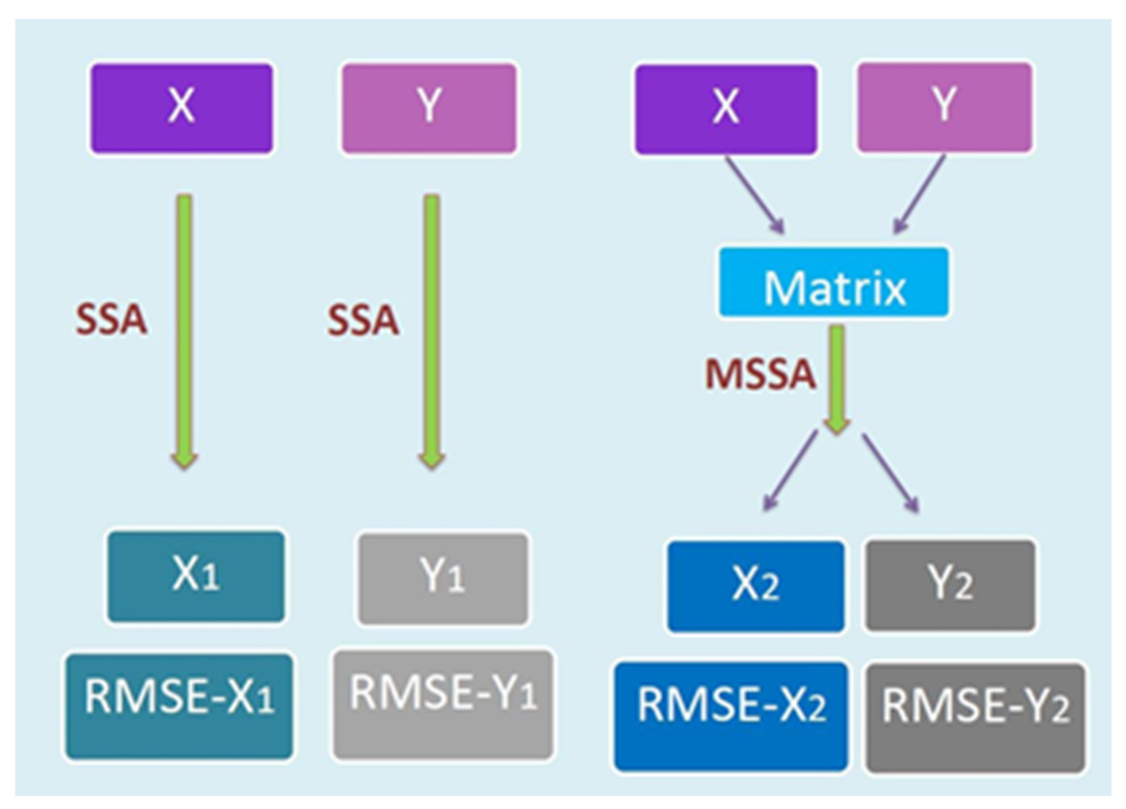
The SSA causality test is based on comparing the forecast performance of the univariate SSA and MSSA with the addition of another variable. As can be seen in Figure 1, if the forecasting performance of X via MSSA after including Y outperforms the univariate SSA forecast performance of X, it indicates that Y contains helpful information for better predicting X, which is then concluded to be a causal relationship.

Figure 1. Flowchart of SSA causality test (Source: Huang et al. 2019). Note: This diagram shows the flowchart of the causality test. From comparing the forecast values obtained by the univariate SSA and multivariate SSA (MSSA) against the actual, if the forecasting errors using MSSA are significantly smaller than those obtained from a univariate SSA, a causal relationship is inferred.

For each series, there are two forecasting values, one by SSA and one by MSSA, after adding another series. Each series can be split into two parts, in and out of the sample series, where the in-sample series is used for performing SSA and MSSA forecasting, whilst the out of sample part is used for calculating and comparing the forecasting error. For a simple two-series case demonstration, namely, series X and Y, the criterion $F_{X|Y}$ of the SSA causality test refers to the prediction performance (root mean square error) of X in the presence of Y, divided by the forecast accuracy of X without Y. Therefore, a smaller index $F_{X|Y}$ indicates that better information is provided by Y to forecast X. In general, if $F_{X|Y}<1$, we conclude that Y has a causal relationship with X; in the case of $F_{X|Y}\ge 1$, no causal relationship is detected.

3. Descriptive Statistics of the Data

The spot and futures data selected in this paper are collected from the WIND Financial Information Database. This study examines seven high-frequency daily closing prices of soybean, corn, wheat, early rice, soybean meal, rapeseed meal and rapeseed. In all cases our sample period ends in October 2017. However, the early rice data start in April 2009, whereas the rapeseed meal and rapeseed series begin in 2012 and the rest in January 2009. The spot prices were taken nationally. The futures contract (No. 1711) includes No. 1 soybean, soybean meal, rapeseed meal and rapeseed. The futures contract (No. 1801) includes corn and early rice and the wheat futures price come from the wheat contract (No. 1805). In line with the usual convention for financial and economic time series, all series are analyzed in logarithmic form. Figure 2 shows the time series data after the application of the logarithmic transformation. In general, periods of price increase before May 2014 and price decrease after May 2014 are evident in the graphs. Table 2 presents the descriptive statistics for the spot and futures return data. In addition, in order to compare the dynamic changes of the futures market and the spot market before and after the cancellation of the temporary collection and storage policy, summary statistics for the periods before May 2014 and after May 2014 are also given in Table 2. In this table $s_{1t}$,$f_{1t}$,$s_{2t}$,$f_{2t}$ and $s_t$,$f_t$ are the futures and spot prices, and $r_{ft}$,$r_{f1t}$,$r_{f2t}$,$r_{st}$,$r_{s1t}$,$r_{s2t}$ are the returns for the two phases and the entire sampling period, respectively. In Table 2, the first two values are the sample mean and the sample standard deviation. For the logarithmically transformed series, these two values are scaled by 100, and hence, effectively refer to percentage changes in the original series.

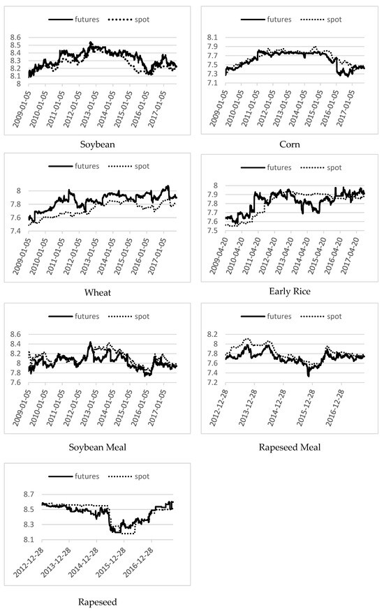
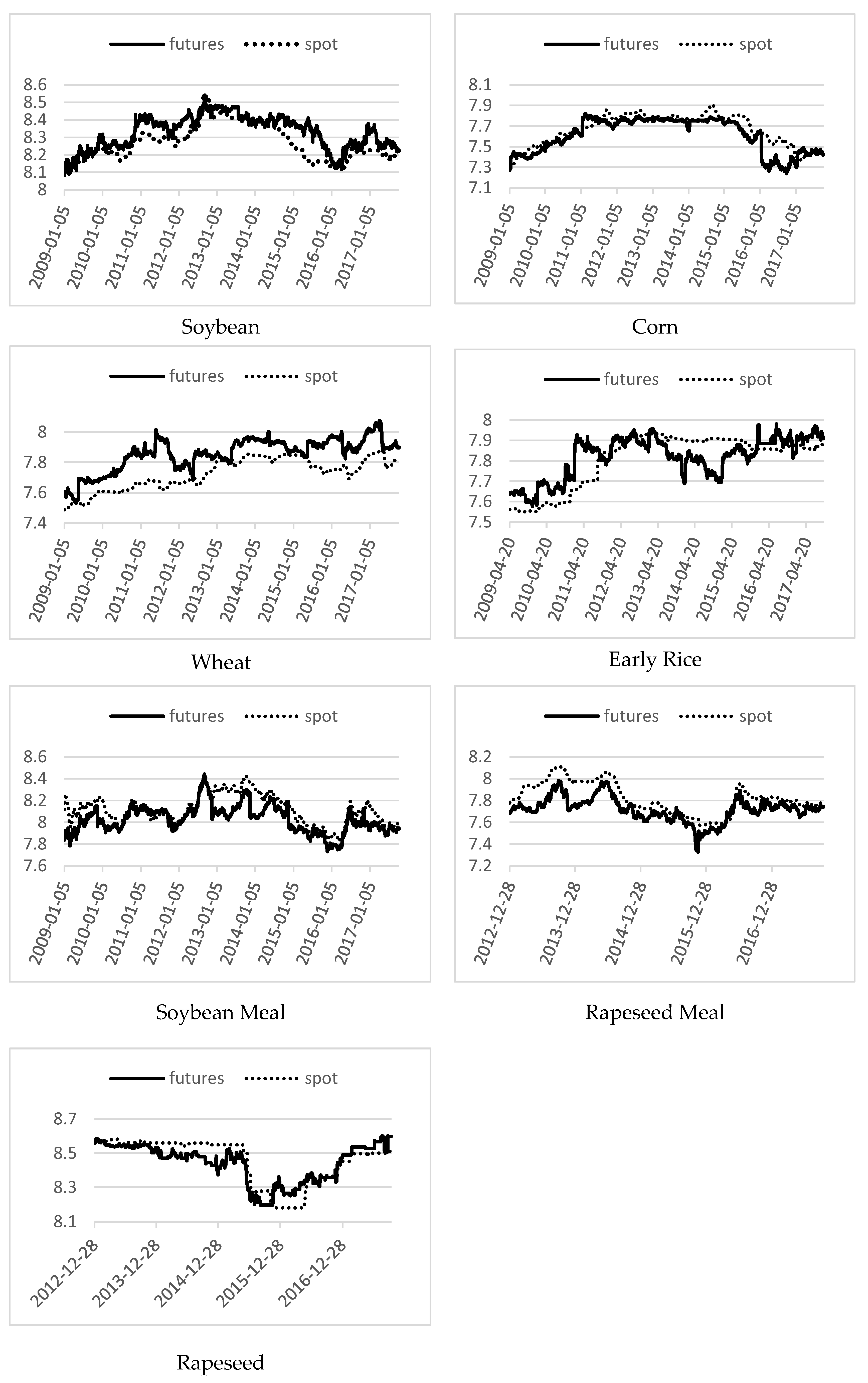
Figure 2. Time series data for seven different spot and futures markets. Note: This figure illustrates the logarithmic transformed time series of futures prices and spot prices for soybean, corn, wheat, early rice, soybean meal, rapeseed meal and rapeseed in solid lines and dashed lines, respectively.

Table 2. Descriptive statistics of the returns of agricultural products.

Commodity	Return	Mean	Standard Deviation	Commodity	Return	Mean	Standard Deviation
Soybean	$r_{ft}$	0.0066	0.9836	Wheat	$r_{ft}$	0.0139	0.8829
	$r_{f1t}$	0.0246	0.9999		$r_{f1t}$	0.0298	0.9104
	$r_{f2t}$	−0.0206	0.9586		$r_{f2t}$	−0.0097	0.8403
	$r_{st}$	0.0021	0.5147		$r_{st}$	0.0157	0.2183
	$r_{s1t}$	0.0167	0.5930		$r_{s1t}$	0.0268	0.1931
	$r_{s2t}$	−0.0202	0.3637		$r_{s2t}$	−0.0011	0.2509
Corn	$r_{ft}$	0.0070	1.0232	Early Rice	$r_{ft}$	0.0135	0.9612
	$r_{f1t}$	0.0380	0.9021		$r_{f1t}$	0.0150	0.9501
	$r_{f2t}$	−0.0400	1.1832		$r_{f2t}$	0.0104	0.9775
	$r_{st}$	0.0076	0.2401		$r_{st}$	0.0157	0.2694
	$r_{s1t}$	0.0370	0.1766		$r_{s1t}$	0.0286	0.31727
	$r_{s2t}$	−0.0375	0.3074		$r_{s2t}$	−0.0027	0.1798
Soybean Meal	$r_{ft}$	0.0048	1.5151	Rapeseed	$r_{ft}$	0.0027	1.1097
	$r_{f1t}$	0.0261	1.4567		$r_{f1t}$	−0.0302	0.6622
	$r_{f2t}$	−0.0275	1.6013		$r_{f2t}$	0.0142	1.2380
	$r_{st}$	−0.0061	0.8365		$r_{st}$	−0.0044	0.7086
	$r_{s1t}$	0.0118	0.9293		$r_{s1t}$	−0.0003	0.1671
	$r_{s2t}$	−0.0336	0.6706		$r_{s2t}$	−0.0059	0.8257
Rapeseed Meal	$r_{ft}$	0.0035	1.5013
	$r_{f1t}$	0.0651	1.3102
	$r_{f2t}$	−0.0181	1.5703
	$r_{st}$	0.0002	0.6083
	$r_{s1t}$	0.0753	0.4473
	$r_{s2t}$	−0.0284	0.6573

Note: This table illustrates the summary statistics of the returns in terms of means and standard deviations for the periods before May 2014 and after May 2014. In this table, $s_{1t}$, $f_{1t}$, $s_{2t}$, $f_{2t}$ and $s_t$, $f_t$ are the futures and spot prices, and $r_{ft}$, $r_{f1t}$, $r_{f2t}$, $r_{st}$, $r_{s1t}$, $r_{s2t}$ are the returns for the two phases and the entire sampling period, respectively. The means and standard deviations are scaled by 100.

Table 2 shows that before the release and cancellation of the policy of temporary storage of agricultural products under the new national 9th Article, the prices both in the futures and in the spot markets, except rapeseed, experienced growth over this period. However, the future and spot prices for all the commodities, except early rice and rapeseed, experienced substantial decline after the release and cancellation of the 9th Article policy. This means that after the issuance of documents and policies, both in the futures market and the spot market, the returns of agricultural products in China have generally decreased. In particular, corn shows an average decline of 0.0400% and 0.0375% per day in the futures and sport markets. Over the sample period, all the futures markets for, soybeans, corn, wheat, soybean meal and rapeseed meal fell more than 50 percent, while the returns on rice futures fell by approximately 11 percent. For all the seven agricultural commodities, the sample standard deviations indicate substantially greater volatility for the futures prices than those of the spot prices. For the futures prices, soybean meal has the highest and wheat has the lowest volatility for the entire sample period. The negative returns for the spot market of all seven commodities after May 2014 indicate that the spot prices of agricultural products in China have all declined. The phasing-out of the temporary storage policy has meant that the government no longer intervenes directly in the price of agricultural products, and the decline in prices for some agricultural products has been caused by the change in government policy. However, the imbalance between supply and demand was the main cause of the decline in the price of agricultural products after May 2014 in China.

4. Empirical Results

4.1. Test of Stationarity and Co-Integration

The Augmented Dickey Fuller test proposed by Dickey and Fuller (2006) is used here to test for the presence of the unit root in the future and spot prices of seven agricultural products.

$$\Delta p_{t }=\rho p_{t-1}+{\displaystyle \sum }_{i=1}^k{p}_{t-1}+v_t$$

(19)

where $\Delta$ is a first difference operator and $v_t$ is a white noise process, and k denotes the lag order. In this paper, the maximum lag order recommended by Schwert (1989) is adopted: $n_{max}=\left[12\ast {\left(\frac{T}{100}\right)}^{\frac{1}{4}}\right]$. Table 3 presents the results of the ADF tests (p-values). It is found that the data for the seven time series for the futures and spot prices are non-stationary, and the first differenced time series is stationary; that is, all of them are I(1) processes.

Table 3. Unit root test and co-integration.

	Unit Root Test				Test of Co-Integration
	${\mathit{f}}_{\mathit{t}}$	$\mathbf{d}{\mathit{f}}_{\mathit{t}}$	${\mathit{s}}_{\mathit{t}}$	$\mathbf{d}{\mathit{s}}_{\mathit{t}}$	Trace Statistics
					r = 0	r = 1
Soybean	0.171	<0.001	0.506	<0.001	22.122	1.440 *
Corn	0.303	<0.001	0.355	<0.001	39.502	3.944 *
Wheat	0.049	<0.001	0.207	<0.001	20.329	5.590 *
Early Rice	0.147	<0.001	0.295	<0.001	16.599	3.598 *
Soybean Meal	0.065	<0.001	0.258	<0.001	33.604	3.719 *
Rapeseed Meal	0.166	<0.001	0.243	<0.001	27.496	1.659 *
Rapeseed	0.631	<0.001	0.567	<0.001	19.958	1.827 *

Note: This table shows the test of unit root and co-integration for the seven agricultural commodities using the maximum lag order recommended by Schwert (1989) $n_{max}=\left[12\ast {\left(\frac{T}{100}\right)}^{\frac{1}{4}}\right]$. The * shows significance at 5%. $f_t$ is the future price at time t. $d{f}_t=f_t-f_{t-1}$ is the change in the futures prices in terms of the first difference. $s_t$ is the spot price and $d{s}_t=s_t-s_{t-1}$ is the first difference of the spot price.

The co-integration test established by Johansen (1988) and Johansen and Juselius (1990) was applied. VAR models are used to establish the trace statistics and maximum eigenvalues to test the long-run relationships between a pair of time series. The test results show that, overall, they are all co-integrated, which indicates that there are long-run equilibrium relationships between the spot and futures markets for agricultural products in China.

4.2. Granger Causality Test

In order to investigate whether there exists causality between the futures market and the spot market, the Granger causality test was computed and the test results are shown in Table 4.

Table 4. Granger causality test.

	Futures Market	Spot Market
Soybean	Futures price Granger causes spot price	Spot price Granger causes futures price
	(0.007)	(0.013)
Corn	Futures price Granger causes spot price	Spot price Granger does not cause futures price
	(0.000)	(0.578)
Wheat	Futures price Granger does not cause spot price	Spot price Granger does not cause futures price
	(0.117)	(0.131)
Early Rice	Futures price Granger causes spot price	Spot price Granger does not cause futures price
	(0.064)	(0.498)
Soybean Meal	Futures price Granger causes spot price	Spot price Granger does not cause futures price
	(0.000)	(0.1263)
Rapeseed Meal	Futures price Granger causes spot price	Spot price Granger does not cause futures price
	(0.000)	(0.134)
Rapeseed	Futures price Granger causes spot price	Spot price Granger does not cause futures price
	(0.000)	(0.273)

Note: This table shows the results of the Granger causality test from the future price on the spot market and the spot price on the futures price. The p-values in the Granger causality test are reported in parentheses.

The results indicate that there is no causality effect between the wheat futures and the spot prices at the 10% significance level. For the other six commodities, the results show that the futures prices have impacts on the spot prices and, except for soybean, that there is mutual causation.

4.3. SSA-Based Causality Test

In this section, in order to further discover the relationship between the agricultural futures and agricultural spot prices in China, a non-parametric causality test based on the Singular Spectrum Analysis method is employed.

The Singular Spectrum Analysis (SSA) method is a modern, powerful, non-parametric decomposition and forecasting model (Beneki et al. 2012) that filters noise and forecasts signals (Hassani et al. 2015). The advantages of SSA over traditional time series models are that it is one of the few models capable of handling non-stationarity and non-normality (Hassani et al. 2015), handling and forecasting missing values (Hassani et al. 2020), and managing other complex characteristics in time series. Univariate SSA, which uses the recurrent and vector techniques, and the multivariate versions of SSA have been applied in forecasting in tourism, economics, fashion and other fields (Silva et al. 2017, 2019; Hassani et al. 2018). Given its wide implementation and success, the design of the SSA causality test is, to the author’s knowledge, for the first time introduced here to study the causality relationship between the spot and futures markets.

There is no specific limitation about the length of out-of-sample, just a general consideration for a simulation scenario, where the length of time series for reconstruction will take two-thirds of the whole series, with the rest used for calculating the forecasting error. In order to conduct the SSA causality test for the futures and spot prices, the out-of-sample size for testing is also set as one-third of the corresponding tested series; the specific series lengths and cutting points are listed in Table 5. Please note that all the forecasting results for both the SSA and multivariate SSA steps are the optimal choice chosen after considering all possible window lengths L and the corresponding choices of the number of eigenvalues r, respectively. For achieving a comprehensive comparison, we conducted SSA causality tests for the total period sample as well as before and after the cancellation of the temporary collection and storage policy periods. As can be seen in Table 5 below, causalities are detected from future price to spot price for the total period sample of more than half of the commodities. It is also noticed that before the cancellation of the temporary collection and storage policy, we detected strong bidirectional causality relationships between the future and spot prices for five commodities, and unidirectional causality from the future to spot price for the other two commodities. After the policy was implemented, although the causality from the future to the spot price shows a diminishing trend based on the results of four commodities, causality from the spot to future price remains for six out of seven commodities apart from soybean meal.

Table 5. SSA causality test.

Commodity	Period	No. of Obs.	Cut Point	Univariate SSA of Futures Price		Univariate SSA of Spot Price		MSSA of Futures Price by Adding Spot Price		SSA Causality Spot Price to Futures Price		MSSA of Spot Price by Adding Futures Price		SSA Causality Futures Price to Spot Price
				L, R	RMSE	L, R	RMSE	L, R	RMSE	F Stat	Decision	L, R	RMSE	F Stat	Decision
Soybean	Total	2126	1416	2, 1	0.010	2, 1	0.006	2, 1	0.011	1.102	NO	2, 1	0.004	0.756	YES
	Before	1285	857	2, 1	0.010	2, 1	0.007	2, 1	0.009	0.886	YES	2, 1	0.006	0.941	YES
	After	841	561	2, 1	0.012	2, 1	0.004	2, 1	0.011	0.923	YES	2, 1	0.004	1.033	NO
Corn	Total	2117	1412	2, 1	0.011	3, 2	0.002	2, 1	0.015	1.298	NO	3, 2	0.003	1.210	NO
	Before	1276	851	2, 1	0.010	4, 2	0.002	2, 1	0.007	0.716	YES	4, 2	0.001	0.830	YES
	After	841	561	2, 1	0.016	3, 2	0.003	2, 1	0.012	0.738	YES	3, 2	0.003	1.004	NO
Wheat	Total	2107	1404	2, 1	0.010	3, 2	0.002	2, 1	0.010	1.015	NO	3, 2	0.003	1.175	NO
	Before	1266	844	2, 1	0.011	4, 2	0.002	2, 1	0.007	0.656	YES	3, 2	0.002	0.711	YES
	After	841	561	2, 1	0.010	3, 2	0.003	3, 2	0.010	0.986	YES	3, 2	0.003	0.922	YES
Early Rice	Total	2033	1355	2, 1	0.010	2, 1	0.002	2, 1	0.011	1.136	NO	2, 1	0.002	0.968	YES
	Before	1192	795	2, 1	0.011	2, 1	0.004	2, 1	0.009	0.838	YES	2, 1	0.002	0.469	YES
	After	841	561	2, 1	0.011	2, 1	0.002	2, 1	0.011	0.985	YES	2, 1	0.002	1.094	NO
Soybean Meal	Total	2124	1416	2, 1	0.017	2, 1	0.009	2, 1	0.018	1.051	NO	2, 1	0.009	0.941	YES
	Before	1283	855	2, 1	0.016	2, 1	0.010	2, 1	0.019	1.206	NO	2, 1	0.009	0.946	YES
	After	841	561	2, 1	0.017	3, 2	0.009	2, 1	0.018	1.042	NO	3, 2	0.007	0.826	YES
Rapeseed Meal	Total	1155	770	2, 1	0.018	4, 2	0.008	2, 1	0.017	0.960	YES	4, 2	0.009	1.208	NO
	Before	314	209	2, 1	0.017	4, 2	0.005	2, 1	0.009	0.522	YES	3, 2	0.004	0.672	YES
	After	841	561	2, 1	0.020	4, 2	0.008	2, 1	0.017	0.894	YES	4, 2	0.009	1.114	NO
Rapeseed	Total	1156	770	2, 1	0.014	2, 1	0.010	2, 1	0.013	0.934	YES	2, 1	0.008	0.807	YES
	Before	315	210	2, 1	0.008	2, 1	0.001	2, 1	0.010	1.274	NO	2, 1	0.000	0.168	YES
	After	841	561	2, 1	0.014	2, 1	0.009	2, 1	0.013	0.960	YES	2, 1	0.006	0.625	YES

Note: This shows the SSA causality test results of univariate and multivariate SSA of the futures price (FP) and spot price (SP). The length of time series for reconstruction takes 2/3 of the whole series and the remaining 1/3 is used for calculating forecasting error. The specific series lengths and cutting points are listed under the column “cut point”. All the forecasting results of both the SSA and MSSA steps are the optimal choice chosen after considering all possible window lengths L and their corresponding choices of the number of eigenvalues r, respectively. For achieving a comprehensive comparison, we conducted SSA causality tests for the total period sample, as well as before and after the cancellation of the temporary collection and storage policy periods.

4.4. Information Share Model

Using the sample data described in the previous section, first the adjustment coefficient vectors in (4) and (5) and the Cholesky decomposition matrix in (13) were estimated. (The detailed VECM estimation results and the Cholesky decomposition matrix are available from the authors upon request.) Then, the price discovery ratios of the futures and spot markets for the seven agricultural products were computed. The average and upper and lower bounds are shown in Table 6.

Table 6. Information shares between spot and future prices.

	Futures Market			Spot Market
	Upper Bound	Lower Bound	Mean	Upper Bound	Lower Bound	Mean
Soybean	13.78	9.10	11.44	90.90	86.22	88.56
Soybean Meal	73.53	35.55	54.54	64.45	26.47	45.46
Corn	99.07	98.36	98.72	1.64	0.93	1.28
Wheat	17.06	15.80	16.43	84.20	82.94	83.57
Early Rice	59.31	58.81	59.06	41.19	40.69	40.94
Rapeseed Meal	62.40	31.46	46.93	68.54	37.60	53.07
Rapeseed	98.63	96.57	97.60	3.43	1.37	2.40

Note: the price discovery ratio (percent) of the futures and spot markets for the seven agricultural products; mean = (upper bound +lower bound)/2. For consistency, we removed the percentage sign from the table.

The information share in Table 6 measures the relative importance of new information in the futures and spot markets to the total variance of VECM. In the futures market, five of the seven products have upper bounds above 50%—corn, early rice, soybean meal, rapeseed meal and rapeseed—with lower bounds of more than 50% for corn, rapeseed and rice. In contrast, the soybean and wheat futures have upper bounds of only 13.78% and 17.06%, with insignificant short-term parameters, indicating that the futures market for these commodities has no impact on the spot market.

The Information Share Model of Joachim Grammig and Franziska J. can give more accurate results and provide more reliable information about the market characteristics to investors and policy-makers. Using the GAUSS software and the constrained maximum likelihood method, the relevant parameters of the Information Share Model are obtained from (18) and are reported in Table 7.

Table 7. Information shares between future and spot prices.

	IST1	IST2	IST
Soybean	58.81	0.75	15.14
Soybean Meal	85.10	71.86	85.11
Corn	86.87	92.47	99.62
Wheat	1.02	82.42	36.99
Early Rice	88.03	28.39	86.26
Rapeseed Meal	69.97	80.29	58.43
Rapeseed	22.75	99.60	99.72

Note: This table shows the price discovery ratio of the futures and spot markets for the seven agricultural products. IST1 shows the information share before 2014; IST2 shows the information share after 2014 and IST is the information share from 2009 to 2017.

The results for information share in Table 7 are in line with previous results reported in Table 6. As can be seen from the results covering 2009 to 2014, the futures prices of soybean meal, corn, early rice, rapeseed meal and rapeseed all have information shares of more than 50%. Similar to the previous results, corn and rapeseed again have the highest contributions and the futures prices of soybeans and wheat have the least effect on the market information share. The results also indicate significant improvements in information shares in wheat and rapeseed after implementation of the 9th Article in May 2014.

4.5. Impulse Response

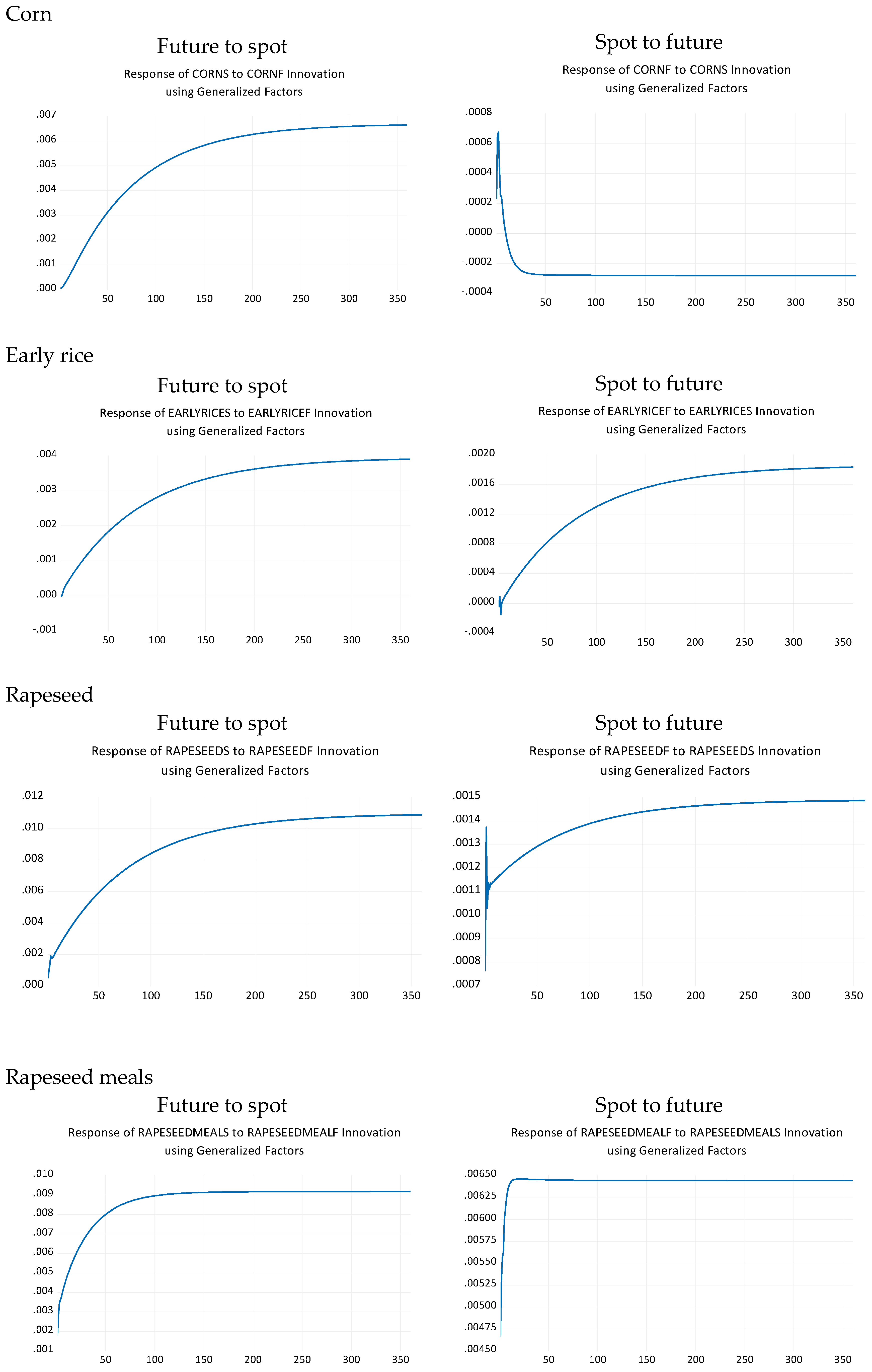
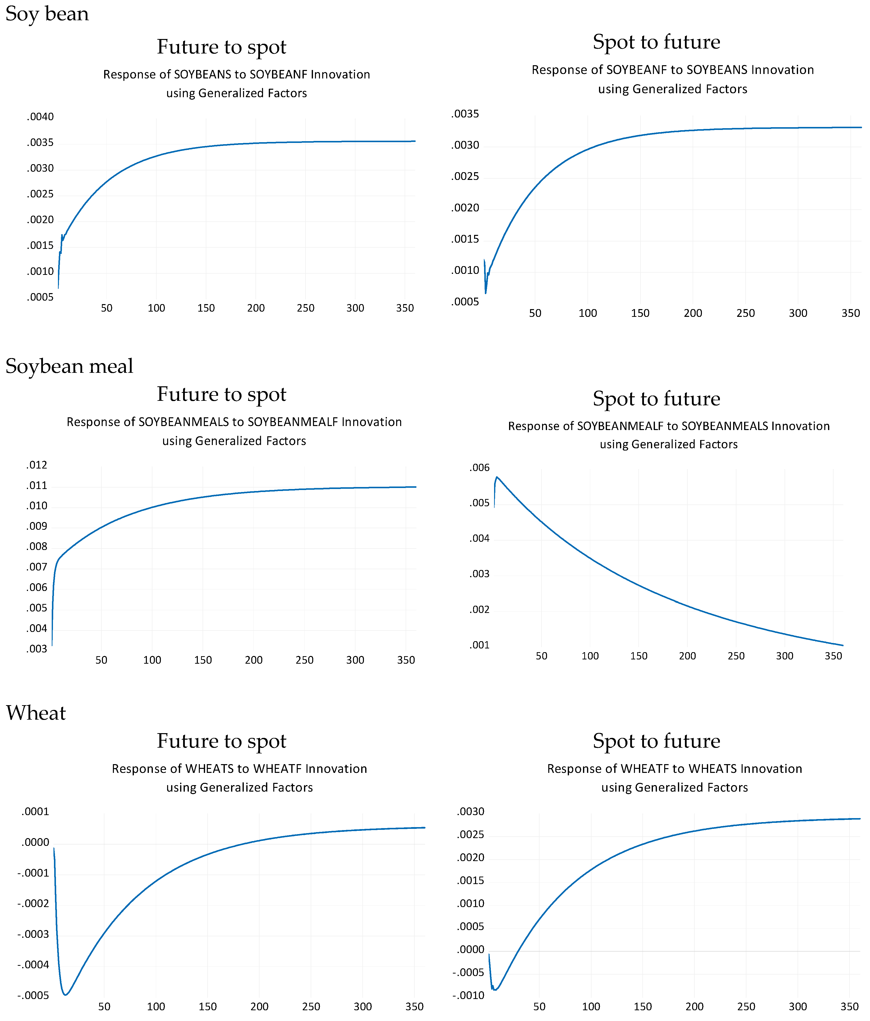
In order to further investigate the contribution of the futures and spot prices of agricultural products to market information, the impulse response functions were computed and analyzed for a period of 360 days. Figure 3 presents the responses of the two markets to shocks of one standard deviation from the other. There are a number of notable points. First, for all the commodities except wheat, a one standard deviation shock from the futures market results in a permanent change in the spot price, showing an increasing reaction in the first three months and then reaching a steady state. For the wheat market, the shock does not have a significant effect and converges to zero after the first three months, which is in line with the results obtained for information share and the causality test for wheat. Second, for all the markets except soybean, the reaction to a one-unit shock of spot prices on futures prices is much smaller and has no significant impact on future prices. For the case of soybean, the impact of a shock on the futures to spot prices, and vice versa, is similar, increasing in the first three months and then converging to 0.0035. This is in line with the results reported in Table 4, showing mutual causality for soybean.

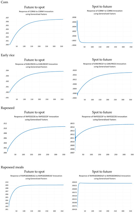
Figure 3. Impulse response function for a duration of 360 days. Note: Figure 3 illustrates the per unit shock of one market on the other of the same product in the form of an impulse response funtion (i.e., future to spot and spot to future) for 360 time periods (days). The seven commodities include corn, early rice, rapeseed, rapeseed meals, soybean, soybean meal and wheat.

Overall, the results of the Impulse Response Function (IRF) presented in Figure 3, show that the spot prices react faster to shocks from the futures market. This confirms our findings reported for the causality tests and the information share analysis. Our results are also consistent and in line with results previously reported by Hua and Liu (2010) and He et al. (2011).

5. Concluding Remarks

In this study, we employed a non-parametric causality test based on Singular Spectrum Analysis (SSA) and used the Vector Error Correction Model (VECM) and two different versions of the Information Share Model (IS) to measure the relationship between the futures and spot prices for seven major agricultural commodities in China from 2009 to 2017. Overall, we found that the futures market in China has potential leading information in price discovery. According to Table 6 and Table 7 and applying the Hasbrouck Information Share Model and the Joachim Grammig and Franziska models, the information share ratios for corn, rapeseed, early rice and soybean meal futures markets are above 50%. This suggests that these futures markets lead the spot market for these products throughout the sample period. There is relatively weak price discovery for the soybean and wheat futures markets. The SSA and Granger causality tests are generally consistent and confirm that, except for wheat and soybean meal, the futures market in China does cause and lead the spot market. In addition, the results of the Impulse Response Function (IRF) show that the spot prices generally react faster to shocks from the futures market and have a lasting impact. This confirms our findings reported for the causality tests and the information share analysis. We also found, generally, that the futures prices provided better information for the spot prices for the agricultural commodity after the new national 9th Article. To achieve the full potential and to establish a developed futures market in China, it is vital that the government in China gradually relaxes the regulations and intervention in the market. They should also initiate and facilitate a self-regulating mechanism for the market and further improve the trading system. Future research directions include extending the time period to explore the potential relationships between agricultural commodities markets during the COVID-19 period and beyond. Furthermore, we can broaden the scope of our study to include less-traded commodities and to compare across countries.

References

- Alexakis, Christos, Guillaume Bagnarosa, and Michael Dowling. 2017. Do cointegrated commodities bubble together? the case of hog, corn, and soybean. Finance Research Letters 23: 96–102. [Google Scholar] [CrossRef]
- Ali, Jabir, and Kriti Bardhan Gupta. 2011. Efficiency in agricultural commodity futures markets in India: Evidence from and causality tests. Agricultural Finance Review 71: 162–78. [Google Scholar] [CrossRef]
- Arnade, Carlos, and Linwood Hoffman. 2015. The impact of price variability on cash/futures market relationships. Implications for market efficiency and price discovery. Journal of Agricultural and Applied Economics 25: 491–514. [Google Scholar] [CrossRef]
- Arnade, Carlos, Bryce Cooke, and Fred Gale. 2017. Agricultural price transmission: China relationships with world commodity markets. Journal of Commodity Markets 7: 28–40. [Google Scholar] [CrossRef]
- Baillie, Richard T., G. Geoffrey Booth, Yiuman Tse, and Tatyana Zabotina. 2002. Price discovery and common factor models. Journal of Financial Markets 5: 309–22. [Google Scholar] [CrossRef]
- Beneki, Christina, Bruno Eeckels, and Costas Leon. 2012. Signal extraction and forecasting of the UK tourism income time series: A singular spectrum analysis approach. Journal of Forecasting 31: 391–400. [Google Scholar] [CrossRef]
- Benz, Eva A., and Jördis Hengelbrock. 2008. Price discovery and liquidity in the European CO2 futures market: An intraday analysis. In AFFI/EUROFIDAI, Paris December 2008 Finance International Meeting AFFI-EUROFIDAI. Available online: https://web.archive.org/web/20140124123857id_/http://www.fbv.kit.edu:80/symposium/11th/Paper/04Commodities/Hengelbrock.pdf (accessed on 1 June 2024).
- Breitung, Jörg, and Bertrand Candelon. 2006. Testing for short- and long-run causality: A frequency-domain approach. Journal of Econometrics 132: 363–78. [Google Scholar] [CrossRef]
- Cha, Tingjun, and Jianling Xu. 2016. Multi-dimensional analysis of soybean futures market efficiency. Journal of South China Agricultural University (Social Science Edition) 3: 88–102. [Google Scholar]
- Dickey, David A., and Wayne A. Fuller. 2006. Likelihood ratio statistics for autoregressive time series with a unit root. Econometrica 49: 1057–72. [Google Scholar] [CrossRef]
- Dolatabadi, Sepideh, Morten Orregaard Nielsen, and Ke Xu. 2015. A fractionally cointegrated VAR analysis of price discovery in commodity futures markets. Journal of Futures Markets 35: 339–56. [Google Scholar] [CrossRef]
- Engle, Robert F., and Clive W. J. Granger. 2006. Co-integration and error correction: Representation, estimation, and testing. Econometrica 55: 251–76. [Google Scholar] [CrossRef]
- Fang, Kuangnan, and Zhenzhong Cai. 2012. Research on price discovery function of stock index futures in China. Statistical Study 5: 73–78. [Google Scholar]
- Figuerola-Ferretti, Isabel, and Jess Gonzalo. 2010. Modelling and measuring price discovery in commodity markets. Journal of Econometrics 158: 95–107. [Google Scholar] [CrossRef]
- Fu, Qiang, Yuxing Wang, and Junwei Ji. 2016. Price discovery and volatility spillover effects of mini gold contracts-based on 5-minute high frequency data. International Business (Journal of the University of Foreign Economics and Trade) 2: 101–11. [Google Scholar]
- Gonzalo, Jesus, and Clive Granger. 1995. Estimation of common long-memory components in cointegrated systems. Journal of Business and Economic Statistics 13: 27–35. [Google Scholar] [CrossRef]
- Grammig, Joachim, and Franziska J. Peter. 2013. Telltale tails: A new approach to estimating unique market information shares. Journal of Financial and Quantitative Analysis 2: 439–88. [Google Scholar] [CrossRef]
- Hasbrouck, Joel. 1995. One security, many markets: Determining the contributions to price discovery. The Journal of Finance 50: 175–99. [Google Scholar] [CrossRef]
- Hassani, Hossein, Allan Webster, Emmanuel Sirimal Silva, and Saeed Heravi. 2015. Forecasting US tourist arrivals using optimal singular spectrum analysis. Tourism Management 46: 322–35. [Google Scholar] [CrossRef]
- Hassani, Hossein, Mohammad Reza Yeganegi, Atikur Khan, and Emmanuel Sirimal Silva. 2020. The effect of data transformation on singular spectrum analysis for forecasting. Signals 1: 4–25. [Google Scholar] [CrossRef]
- Hassani, Hossein, Saeed Heravi, and Anatoly Zhigljavsky. 2009. Forecasting European industrial production with singular spectrum analysis. International Journal of Forecasting 25: 103–18. [Google Scholar] [CrossRef]
- Hassani, Hossein, Saeed Heravi, and Anatoly Zhigljavsky. 2013. Forecasting UK industrial production with multivariate singular spectrum analysis. Journal of Forecasting 32: 395–408. [Google Scholar] [CrossRef]
- Hassani, Hossein, Silva Emmanuel, Gupta Rangan, and Sonali Das. 2018. Predicting global temperature anomaly: A definitive investigation using an ensemble of twelve competing forecasting models. Physica A: Statistical Mechanics and its Applications 509: 121–39. [Google Scholar] [CrossRef]
- He, Chengying, Longbin Zhang, and Chen Wei. 2011. Research on price discovery of HS300 index futures based on high frequencies data. Journal of Quantitative and Technical Economics 5: 139–51. [Google Scholar]
- Hou, Jinli. 2014. Study on the relationship between futures price and spot price of agricultural products. The Economy 4: 70–74. [Google Scholar]
- Hua, Renhai, and Qingfu Liu. 2010. The research on price discovery ability between stock index futures market and stock index spot market. Journal of Quantitative and Technical Economics 10: 90–100. [Google Scholar]
- Huang, Xu, Paula Medina Maçaira, Hossein Hassani, Fernando Luiz Cyrino Oliveira, and Gurjeet Dhesi. 2019. Hydrological natural inflow and climate variables: Time and frequency causality analysis. Physica A: Statistical Mechanics and Its Applications 516: 480–95. [Google Scholar] [CrossRef]
- Johansen, Søren, and Katarina Juselius. 1990. Maximum likelihood estimation and inference on cointegration-with application to the demand for money. Oxford Bulletin of Economics and Statistics 52: 169–210. [Google Scholar] [CrossRef]
- Johansen, Søssren. 1988. Statistical analysis of cointegration vectors. Journal of Economic Dynamics and Control 12: 231–54. [Google Scholar] [CrossRef]
- Joseph, Anto, Garima Sisodia, and Aviral Kumar Tiwari. 2014. A frequency domain causality investigation between futures and spot prices of Indian commodity markets. Economic Modelling 40: 250–58. [Google Scholar] [CrossRef]
- Joseph, Anto, Suresh K. G., and Garima Sisodia. 2015. Is the causal nexus between agricultural commodity futures and spot prices asymmetric? Evidence from India. Theoretical Economics Letters 5: 285–95. [Google Scholar] [CrossRef]
- Li, Zheng, Lin Bo, and Yi Hao. 2016. Re-discussion on the function of price discovery of stock index futures in China-empirical evidence from three listed varieties. Economy of Finance and Trade 7: 79–93. [Google Scholar]
- Liang, Quanxi, Guanying Yue, and Jun Chen. 2009. An empirical study on the role of futures market in sugar price formation in China. The Price (monthly issue) 3: 14–17. [Google Scholar]
- Liu, Qingfeng Wilson. 2005. Price relations among hog, corn, and soybean meal futures. Journal of Futures Markets 25: 491–514. [Google Scholar] [CrossRef]
- Liu, Qingfu, and Jinqing Zhang. 2006. A study on the function of price discovery in the futures market of agricultural products in China. Research on Industrial Economic 1: 8. [Google Scholar]
- Schwert, G. William. 1989. Tests for unit roots: A monte carlo investigation. Journal of Business and Economic Statistics 7: 147–59. [Google Scholar] [CrossRef]
- Silva, Emmanuel Sirimal, Hossein Hassani, Saeed Heravi, and Xu Huang. 2019. Forecasting tourism demand with denoneural networks. Annals of Tourism Research 74: 134–54. [Google Scholar] [CrossRef]
- Silva, Emmanuel Sirimal, Zara Ghodsi, Mansi Ghodsi, Saeed Heravi, and Hossein Hassani. 2017. Cross country relations in European tourist arrivals. Annals of Tourism Research 63: 151–68. [Google Scholar] [CrossRef]
- Taunson, Jude W., Mohd Fahmi Bin Ghazali, Minah Japang, and Abd Kamal Bin Char. 2018. Intraday lead-lag relationship between index futures and stock index markets: Evidence from Malaysia. Journal of Modern Accounting and Auditing 14: 561–69. [Google Scholar]
- Tse, Yiuman. 1999. Price discovery and volatility spillovers in the DJIA index and futures markets. Journal of Futures Markets 19: 911–30. [Google Scholar] [CrossRef]
- Wang, Qunyong, and Xiaodong Zhang. 2005. Price discovery function of crude oil futures market-analysis based on Information share model. Statistics and Decision-Making 12: 77–79. [Google Scholar]
- Wang, Yu-Shan, Chung-Gee Lin, and Shih-Chieh Shih. 2011. The dynamic relationship between agricultural futures and agriculture index in China. China Agricultural Economic Review 3: 369–82. [Google Scholar] [CrossRef]
- Xu, Yuanyuan, Fanghui Pan, Chuanmei Wang, and Jian Li. 2019. Dynamic price discovery process of Chinese agricultural futures markets: An empirical study based on the rolling window approach. Journal of Agricultural and Applied Economics 51: 664–81. [Google Scholar] [CrossRef]
- Yao, Chuanjiang, and Fenghai Wang. 2005. Empirical analysis on the efficiency of China’s agricultural futures market: 1998–2002. Research on Financial Issues 1: 43–49. [Google Scholar]
- Zhao, Zhao, and Qiang He. 2015. A dynamic study on the price relationship between copper futures and spot in China. Research on Technology, economy and Management 11: 96–100. [Google Scholar]
Disclaimer/Publisher’s Note: The statements, opinions and data contained in all publications are solely those of the individual author(s) and contributor(s) and not of MDPI and/or the editor(s). MDPI and/or the editor(s) disclaim responsibility for any injury to people or property resulting from any ideas, methods, instructions or products referred to in the content. |
© 2024 by the authors. Licensee MDPI, Basel, Switzerland. This article is an open access article distributed under the terms and conditions of the Creative Commons Attribution (CC BY) license (https://creativecommons.org/licenses/by/4.0/).