Does the Design of Stablecoins Impact Their Volatility?

Abstract

In this paper, we shall compare the average volatility that characterises the main stablecoin design types with a view to answering the question of whether all stablecoin designs accomplish the goal of minimising their price fluctuations to the same degree. Our research is motivated by the lack of rigorous studies comparing volatility of different stablecoin types stressed in the literature as well as the practical importance of such a comparison from the investors’ viewpoint. We opted for a standard volatility measure, i.e., standard deviation of return rates, corrected it for autocorrelation, and detected differences between distributions of the measure in three stablecoin groups using various non-parametric tests, i.e., the Kruskal–Wallis test, the bootstrap F-test, post-hoc tests and non-parametric contrasts. We proved that stablecoins do not deliver equally on the promise to provide stable market value with tokenised funds being leaders. Tokenised funds design involves complete coverage of the stablecoin supply in units of the currency of reference as well as great dependence on the trusted third-party acting as a trustee for the collateral. Our study reveals that existing complex stablecoins designs hardly compete with this simple design in terms of volatility.

1. Introduction

Recently, a new trend has emerged on the cryptocurrency market—transferring funds toward low volatility digital assets, which resulted in a jump in the stablecoin economy (Sidorenko 2020). Currently the most popular stablecoin, Tether, is the third cryptocurrency in terms of market capitalization and the first in terms of daily trading volume1. While many definitions of stablecoins can be found in the literature (especially research studies by the business community (e.g., Blockchain 2018; Samman and Masanto 2019; Sameeh 2018)), in this paper, we choose to follow the definition by Bullmann et al. (2019), which states that stablecoins are digital units of value that are not a form of any specific currency (or basket thereof) but, rather, by relying on a set of stabilization tools, try to minimize fluctuations in their price in such currencies. It is important to note that, by following this definition, we exclude from further consideration most of the so-called gold-backed cryptocurrencies (as presented by Aloui et al. (n.d.)) because the stabilization mechanism they employ is not strictly focused on minimizing price fluctuations. The definition that we have adopted has the distinct advantage of not using terms such as ‘cryptocurrency’ or ’token’, which can be defined in a number of ways, as well as being specific about what makes stablecoins stable2. It stresses that each stablecoin has its currency or basket of currencies of reference.

As commonly discussed (Wei 2018; Calle and Zalles 2019), the key purpose of stablecoins is the conversion and exchange into other cryptocurrencies. Numerous stablecoins proved themselves to be some of the most liquid cryptocurrencies regardless of economic circumstances (Kyriazis and Prassa 2019). The exact number of stablecoins is hard to specify. Only some of the projects are out of the development phase (with the number constantly fluctuating), while some other have already been closed. Stablecoins are a relatively diverse group of initiatives. The differentiating factors include: the blockchain they operate on, revenue models, country of origin or operation, the scale and adoption on cryptoasset exchanges, the type of issuer, and the scope of decentralisation. However, following Bullmann et al. (2019), the most important distinction between different types of stablecoins can be made on the basis of the stabilisation mechanism that is part of their design. Therefore, four categories can be distinguished: tokenised funds, off-chain collateralised stablecoins, on-chain collateralised stablecoins and algorithmic stablecoins. Each group makes use of its unique design to deliver on the promise of maintaining stable market value. While examples of all four types of stablecoins can be found, not all of them are represented equally, with tokenised funds and on-chain collateralised stablecoins being the most numerous categories.

Tokenised funds are stablecoins backed by funds denominated in a single currency or a basket (it serves as the currency or basket of currencies of reference at the same time) thereof that rely on a custodian for safekeeping and maintaining their full redeemability. Off-chain collateralised stablecoins are backed by other traditional asset classes that their price in the currency of reference changes over time. On-chain collateralised stablecoins are backed by cryptoassets recorded directly in a digital form on a distributed ledger without the need for an issuer or custodian to satisfy any claim. The idea behind algorithmic stablecoins involves a computer algorithm balancing the supply and demand for stablecoins in order to maintain price stability in the currency of reference by using a set of secondary stabilisation tools. A more detailed discussion on those mechanisms including risks associated with them can be found in the paper by Bullmann et al. (2019).

As noted by Chohan (2019), whether stablecoins are truly stable is still an unresolved question. Following the growing body of research focused on stablecoins, our work is designed to answer the following question: do all stablecoin designs accomplish the goal of minimising their price fluctuations to the same degree? The aim of the article is to compare the volatility which characterizes the main stablecoin design types. Since stablecoins are being created to minimize price fluctuations in a currency of reference, the volatility is their crucial characteristic that allows the comparison of their performance and assessment of the extent to which they deliver on the promise of maintaining stable market value. As it was stated earlier, the primary objective of including stablecoins in cryptoassets portfolio is to manage cash flows; thus, higher volatility translates into greater probability of a shortfall. Different stablecoin designs utilise different stabilisation mechanisms that imply different risks that investors bear while converting the funds into a particular stablecoin. Only a deep understanding of volatility minimisation and credit and financial risks trade-offs will allow the participants of cryptomarkets to consciously shape their portfolios.

Our approach employs a standard procedure of comparing distributions using the non-parametric Kruskal–Wallis test and the non-parametric bootstrap F-test for comparing more than two groups. We use standard deviation of daily logarithmic returns corrected for autocorrelation as a proxy for volatility. The measure of volatility we opt for is traditional and innovative at the same time since we apply a novelty correction based on ACF function estimator to the standard volatility measure. Our analysis is performed on daily data regarding 20 stablecoins divided into three groups, from their debut (in each case different) until 25 September 2019. Since there is only one representative of off-chain collateralised stablecoins, we decided to aggregate off-chain and on-chain collateralised stablecoins into one group to include all the stablecoins in our research and to enable rigorous and consistent statistical analysis while having in mind that off-chain and on-chain collateralised stablecoins have a lot in common (they are all collateralised and the price of collateral in the currency of reference changes over time; both designs require over-collateralisation and posting extra collateral in response to adverse market movements, i.e., margin calls). The span of datasets ranges from 30 to 1893 observations, depending on the stablecoin. Our study proves that various types of stablecoins, differentiated on the basis of the stabilisation mechanism they employ as part of their design, are not volatile to the same extent. We were not able to create a ranking, but we can confidently state that tokenised funds are the stablecoin design type that displays lower volatility than the other types.

The volatility of bitcoin and other cryptocurrencies has been a popular subject of study over the last decade (e.g., Dwyer 2015; Katsiampa 2017, 2019; Koutmos 2018; Ardia et al. 2019). The volatility of stablecoins has not been studied as thoroughly (as noted by Chohan 2019). The main claim on which stablecoins are founded needs to be tested by analysing the historical volatility of stablecoins and reported not only alongside that of bitcoin but compared among all stablecoin types. We intend to contribute to that branch of research by expanding and statistically testing the findings made by Bullmann et al. (2019). The research done by Bullmann et al. (2019) uses the annualised seven-day rolling standard deviation of daily logarithmic returns (which, in fact, assumes that rates of return are independent) to assess stablecoin volatility and it does so by comparing only three stablecoins. Our analysis, to the best of our knowledge, is the first one ever to apply rigorous statistical inference to compare the volatility of stablecoins based on design choices. Furthermore, our research is much more exhaustive, covering 20 stablecoins instead of focusing on a representative few. It does not make any unrealistic assumptions about rates of return, either.

In addition to being motivated by the scarce research in the area of stablecoin volatility, our interest lies in the desire to further explore the differences between various stablecoin designs and their consequences. Currently, the most widely researched topic focusing on stablecoins is testing whether stablecoins display the properties of diversifiers, hedges or safe havens (e.g., Wang et al. 2020; Baur and Hoang n.d.; Aloui et al. n.d.). It is worth noting that Baur and Hoang (n.d.) identify a trade-off between the properties of ‘stable’ and ‘safe haven’, meaning that a strong safe haven property deprives a stablecoin of its ‘stable’ property. Baur and Hoang (n.d.) as well as Wang et al. (2020) confirm that some stablecoins can serve as a safe haven against bitcoin and other assets. Both papers mention, however, the need to further explore the design of stablecoins (Baur and Hoang n.d.) or attempt to explain the differences in results for each stablecoin with differences in their design (Wang et al. 2020). Our work can, therefore, be seen as furthering that line of research through a contribution to the understanding of the determinants of volatility in cryptocurrencies in general and stablecoins in particular. An advantage of the methodology we use is that we can focus only on stablecoins, regardless of other types of assets, as is the case with the line of research into safe havens. Our results are not reported relative to bitcoin or any other type of asset, which makes the results much less dependent of the market conditions in which stablecoins find themselves.

The remainder of this paper is organised as follows. Section 2 describes the data and methodology of the research, while Section 3 presents empirical results. Section 4 is a discussion of the results and Section 5 concludes.

2. Materials and Methods

All the stablecoins as listed by Bullmann et al. (2019), that were operational as of the cut-off date and whose quotations were available on coinmarketcap.com, are included in our study. Our dataset includes eight tokenised funds, one off-chain collateralised stablecoin, eight on-chain collateralised stablecoins (hereinafter together called collateralised stablecoins), and three algorithmic stablecoins. Thus, all types of stablecoins are represented, although the number of stablecoins within each group varies.

The raw dataset contains daily prices of 20 stablecoins expressed in USD. In the case of stablecoins pegged to currencies other than USD (Stasis and Terra), exchange rates vis-à-vis USD were used to calculate prices in the currency of reference. The EUR/USD exchange rate was sourced from the European Central Bank’s Statistical Data Warehouse (sdw.ecb.europa.eu), while the price of Special Drawing Rights (SDRs) in USD was sourced from IMF’s website (imf.org). The time-span runs from the individual stablecoin’s debut up to 25 September 2019. The number of observations ranges from 30 to 1893, depending on the stablecoin. Further, daily stablecoin prices are transformed into daily logarithmic returns.

The concept of volatility of a financial instrument refers to dispersion of price changes or return rates of the asset. It is an unobservable market characteristic. While it is possible to observe price movements, it is not possible to observe the instrument’s volatility (Kliber 2010). We can, however, approximate it with statistical models. Some of the measures used to analyse volatility are dynamic, while others are static. The simplest measure of volatility of a financial instrument is the standard deviation of its price. Dynamic measures, such as GARCH and stochastic volatility models, implied volatility models or realised volatility models allow researchers to track changes in volatility. The testing procedure employed in order to detect differences in volatility between groups of stablecoins prompted us to use a static volatility measure. We chose a standard deviation of daily logarithmic rates of return corrected for autocorrelation based on the estimate of ACF function (Zięba and Ramza 2011).

The formula for unbiased estimator of variance while observations are autocorrelated is as follows:

$$s^2=\frac{n_{eff}}{n\left(n_{eff}-1\right)}{\displaystyle \sum }_{t=1}^n{\left(i_t-\overline{i}\right)}^2$$

(1)

where $i_t$ is a daily logarithmic rate of return, $n$ is a number of observations for a given stablecoin, and $n_{eff}$ is an effective number of observations.

To use an estimate of ACF function we opted for procedure introduced by Zhang (2006) that limits lag to the last significant non-zero element of autocorrelation function estimate. Thus, we first computed standard errors of elements ($r_k$) of autocorrelation function estimate:

$$s\left(r_k\right)=\{\begin{array}{cc}\hfill \frac{1}{\sqrt{n}},& k=1\hfill \\ \hfill \sqrt{\frac{1+2{{\displaystyle \sum }}_{j=1}^{k-1}{r}_j^2}{n}},& k\ge 2\hfill \end{array}$$

(2)

Then, the maximum lag is determined by

$$n_c=\max \{k|\left|r_k\right|>1.96s\left(r_k\right)\}$$

(3)

and it is limited to $n/4$

$$n_c=\min \left\{n_c,n/4\right\}$$

(4)

Finally, the formula for estimate of $n_{eff}$ is as follows:

$$\widehat{n_{eff}}=\frac{n-2n_c-1+n_c\left(n_c+1\right)/n}{1+2{{\displaystyle \sum }}_{k=1}^{n_c}{r}_k^2}+1$$

(5)

The next step of our analysis involves testing whether there exists a statistical difference between the stablecoin groups in terms of volatility.

There is a vast number of statistical procedures to test for location effects of more than two groups. ANOVA is a standard parametric procedure to test equality of means across groups. Parametric methods are considered to have greater power compared to non-parametric methods when their assumptions are met. However, if the assumptions of the normal distribution of residuals and homogeneity of variances in the data are not met, one should refrain from using ANOVA (Sheskin 2000). We used the Shapiro-Wilk test (Shapiro and Wilk 1965) and the Kolmogorov-Smirnov test (Sheskin 2000) to test for normality (both the nulls postulate the normality of distribution), as well as the Bartlett test (Bartlett 1937), the Fligner–Killeen test (Fligner and Killeen 1976) and the Levene test (Levene 1960) to test for homogeneity of variances across the groups (all the nulls state variances are homogenous).

If the conditions of ANOVA are not met, then the Kruskal–Wallis test (Kruskal and Wallis 1952) is a standard nonparametric procedure for testing whether two or more independent samples originate from the same distribution. Thus, the null hypothesis states

$$F_1=F_2=\cdots =F_k$$

(6)

and the alternative hypothesis is that:

$$F_i\ne F_j \mathrm{for} \mathrm{at} \mathrm{least} \mathrm{one} \mathrm{pair}.$$

(7)

The test is rank-based, and all the observations are ranked ignoring group membership. A formula for the test statistic is as follows:

$$H=\left(N-1\right)\frac{{{\displaystyle \sum }}_{i=1}^k{n}_i{\left(\overline{l_i}-\widehat{l}\right)}^2}{{{\displaystyle \sum }}_{i=1}^k{{\displaystyle \sum }}_{j=1}^{n_i}{\left(l_{ij}-\widehat{l}\right)}^2}$$

(8)

where $k$ is a number of groups, $N$ is the total number of observations, $n_i$ and $\overline{l_i}$ are the number of observations and a mean of ranks of the $i$-th group, respectively, and $\widehat{l}$ is a global mean of ranks.

An exact distribution of the test statistic under the null requires computing all the ranks’ permutations. However, the distribution of H can be approximated by the chi-squared distribution with $k-1$ degrees of freedom. Since our $n=20$, we decided to use both an asymptotic p-value and exact p-value as reported by Meyer and Seaman (2008).

One of the main limitations of the procedure described above is the fact that a significant result does not differentiate whether the difference is between the location (median) or shape (scale and symmetry) of the distribution if assumptions of an identically shaped and scaled distributions cannot be made (Dwivedi et al. 2017). A significant result in the Kruskal–Wallis test signifies that not all of the distributions are equal. Still, it does not say which groups are different.

To check the robustness of the standard nonparametric method, we decided to employ the bootstrap technique. Some authors reported empirical evidence for a reliable performance of the bootstrap approach for testing with regard to a small sample (Dwivedi et al. 2017; Hall and Martin 1988). To avoid making any assumptions about data distribution, we opted for a nonparametric bootstrap where the population distribution is represented by the sample distribution. The number of resamples in our study is 10,000.

Two important steps when applying the bootstrap method are: selection of a test statistic and selection of the resampling strategy (Dwivedi et al. 2017).

Boos and Brownie (1988) and Dwivedi et al. (2017) used the F statistic for comparing more than two independent means. In contrast to the classical ANOVA procedure, the bootstrap procedure implies using a bootstrap distribution of the test statistic. However, one should bear in mind that bootstrap data have to be generated from a distribution that satisfies the restrictions specified by the null hypothesis, which may exclude the empirical distribution of the original data (if the alternative hypothesis is true). Thus, the original data should be properly transformed to satisfy the null’s requirements if needed (having used the F statistic for comparison of means, we opted for centring the data).

When selecting the resampling strategy, we decided to follow the recommendation of Shao and Tu (1995) who suggest using the location aligned and then combined sample. It implies that, from each datapoint, a respective group mean is deducted at first, then differences are pooled, and bootstrap samples are drawn from this set.

If the global null hypothesis postulated by the appropriate statistical procedure (the Kruskal-Wallis test and nonparametric bootstrap F-test, in our case) is rejected, the analysis must be followed by the so-called post-hoc tests which aim at analysing specific sample pairs. We used well-known multiple rank sum Dunn’s test, (Dunn 1964) with Benjamini and Hochberg correction (Benjamini and Hochberg 1995), and the pairwise Wilcoxon–Mann–Whitney U rank sum test (Sheskin 2000) with Holm’s correction (Holm 1979). All the tests’ p-values are adjusted for multiple comparisons.

Since the tokenised funds mechanism directly refers to the currency of reference and ensures full collateralisation in this currency, we expect tokenised funds to be stable to the greatest extent. Thus, we are interested in testing the specific arbitrary contrast. Standard nonparametric statistical procedures allow for pairwise testing only. Hence, we apply the nonparametric rank-based multiple contrast test procedure, based on generalized relative effects developed by Konietschke et al. (2012), which allows the examination of transitive relative effects in the unbalanced one-way design with independent observations, a fixed number of levels, and arbitrary contrasts. Under the null hypothesis, the distributions can have different shapes; in particular, the procedure does not assume homogeneous variances. The general model specifies that:

$$X_{ik}~F_i,k=1,\dots ,n_i$$

(9)

and the generalized relative effects are defined by:

$$p_j=\int Gd{F}_j,j=1,\dots ,a$$

(10)

where $G={\displaystyle \sum }_{i=1}^a{w}_i{F}_i$ denotes a mean distribution in its unweighted form ($w_i=1/a$). If $p_i<p_j$, then values from $F_i$ tend to be smaller than values from $F_j$. It should be noted that $p_j$ is a linear combination of pairwise relative effects $p_{ij}$, i.e.,

$$p_j={\displaystyle \sum }_{i=1}^a{w}_i{p}_{ij},j=1,\dots ,a$$

(11)

where $p_{ij}=\int F_{i}d{F}_j$.

Now let $𝕡={\left(p_1,\dots ,p_a\right)}^{\prime }=\int Gd\mathbb{F}$, where $\mathbb{F}$ is a vector of distributions. The family of hypotheses tested refers to the generalized relative effects and contrast matrix:

$${\mathsf{\Omega }}^p=\left\{H_0^p:c_l^{\prime }𝕡=0,l=1,\dots ,q\right\}$$

(12)

Our contrast matrix consists of pairwise comparisons (Dunn’s contrasts) and one extra contrast which tests whether the relative effect of tokenised funds is equal to the average effect of the remaining stablecoin types.

Rank estimators of $p_j$ are computed by replacing the unknown distribution functions by their empirical counterparts ${\widehat{F}}_i\left(x\right)=1/n_i{\displaystyle \sum }_{k=1}^{n_i}c\left(x-X_{ik}\right),i=1,\dots ,a$, where $c\left(x\right)=1,1/2,1$ for $x<0,x=0,x>0$, respectively. Then, pairwise relative effects are estimated by:

$${\widehat{p}}_{ij}=\int {\widehat{F}}_{i}d{\widehat{F}}_j=\frac{1}{n_j}{\displaystyle \sum }_{k=1}^{n_j}{\widehat{F}}_i\left(X_{jk}\right)=\frac{1}{n_i}({\overline{R}}_{j.}^{\left(ij\right)}-\frac{n_j+1}{2})$$

(13)

where ${\overline{R}}_{j.}^{\left(ij\right)}$ is a mean of the ranks in sample $j$. Finally, the estimator of $p_j$ is obtained as a linear combination of ${\widehat{p}}_{ij}$.

The test procedure includes first deriving the test statistic for each individual hypothesis $H_0^p:c_l^{\prime }𝕡=0$, i.e.,

$$T_l^p=\frac{\sqrt{N}{c}_l^{\prime }\left(\widehat{p}-p\right)}{\sqrt{c_l^{\prime }\widehat{V_N}{c}_l}},l=1,\dots ,q$$

(14)

where $\widehat{V_N}$ is the asymptotic covariance matrix (cf. Konietschke et al. (2012) for derivation details). The test statistic follows asymptotically $N\left(0,1\right)$. The vector of the test statistics $\mathbb{T}={\left(T_1^p,\dots ,T_q^p\right)}^{\prime }$ has asymptotically standard normal distribution as $N\to \infty$ (cf. Konietschke et al. (2012) for derivation details).

The statistics are tested using multivariate t-distribution. We assumed a standard 5% familywise error level.

We relied on the R project for statistical computing (including packages multcomp, FSA, and nparcomp).

3. Results

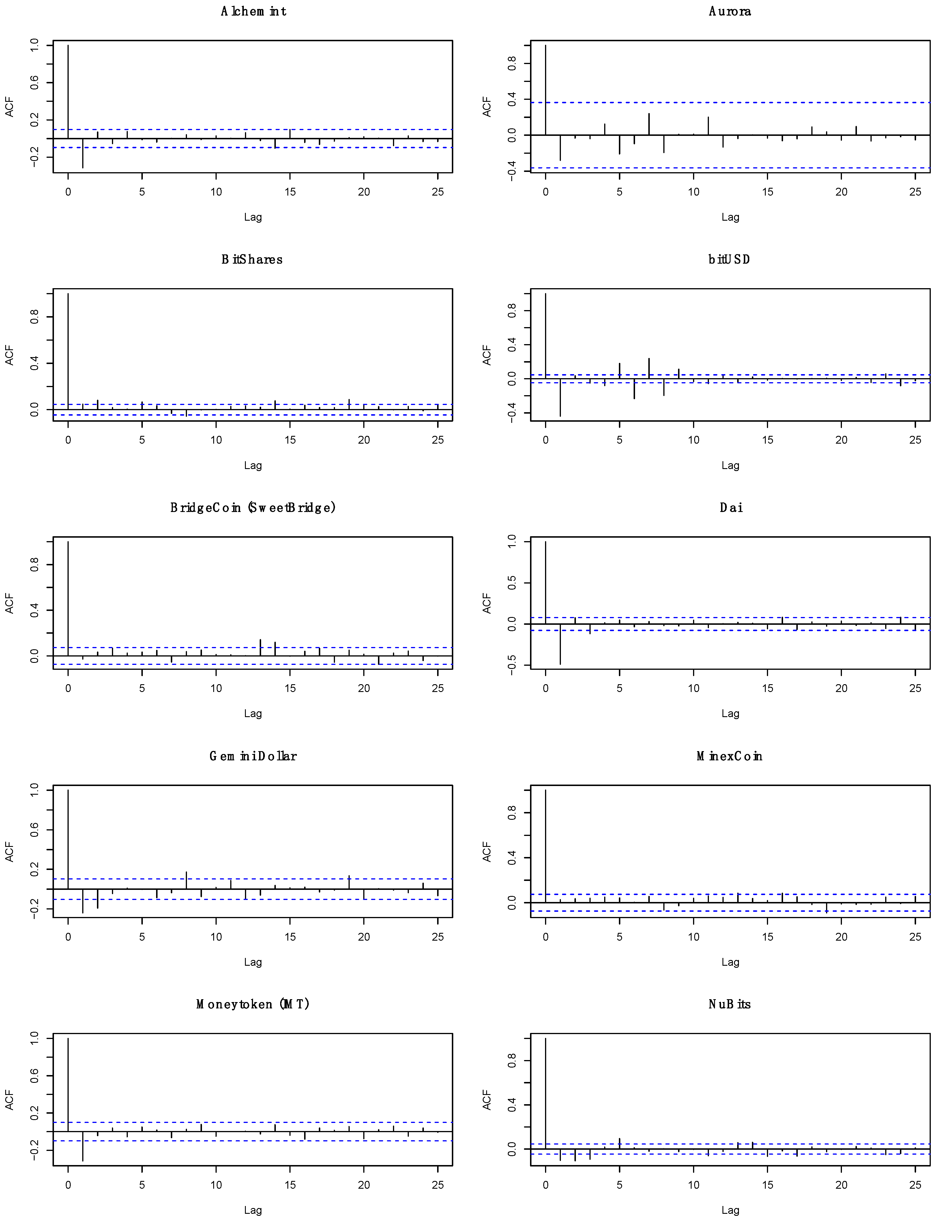
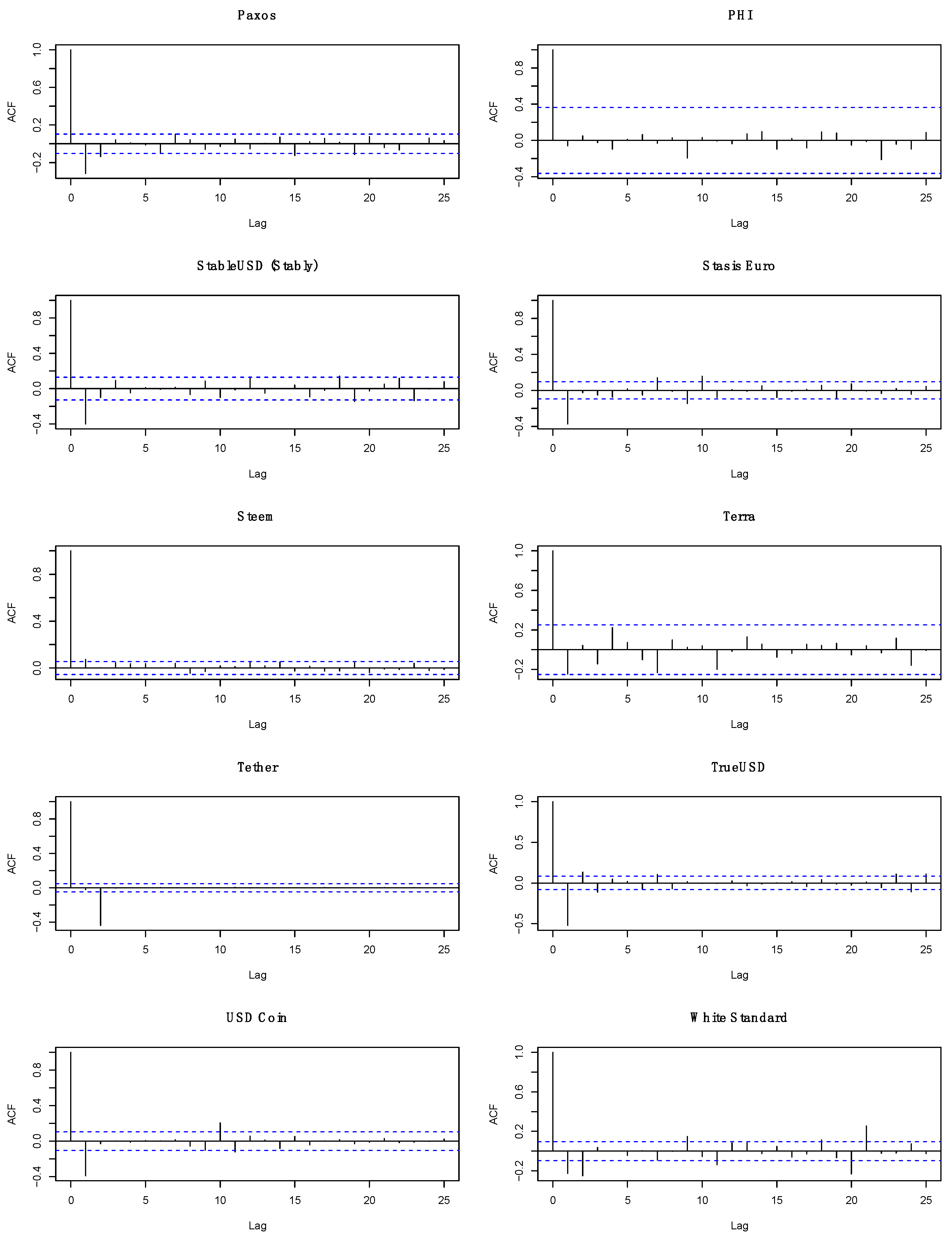
The first step of our analysis was to compute a static measure of volatility, i.e., the autocorrelation-corrected standard deviation (hereinafter SD) of daily log returns, and to perform a statistical test to detect potential differences in the location effects between groups. Figure 1 presents estimates of ACF function for the stablecoins. A quick look at the graphs reveals that the correction of SD for autocorrelation is necessary.

Table 1. A ranking of 20 stablecoins included in the study according to the SD of daily returns (in percentage points).

Name	Peg	Volatility (in p.p.)	Type
Paxos	USD	0.457619	tokenised funds
USD Coin	USD	0.552184	tokenised funds
StableUSD (Stably)	USD	0.640032	tokenised funds
TrueUSD	USD	0.770574	tokenised funds
Gemini Dollar	USD	1.194509	tokenised funds
Dai	USD	1.48214	collateralised (on-chain)
Stasis Euro	EUR	1.510869	tokenised funds
Tether	USD	2.165575	tokenised funds
Terra	SDR	3.956304	algorithmic
Aurora	USD	6.762596	collateralised (on-chain)
PHI	USD	7.334355	collateralised (on-chain)
BitShares	USD	7.444987	collateralised (on-chain)
NuBits	USD	8.58101	algorithmic
Moneytoken (IMT)	USD	9.119281	collateralised (on-chain)
Steem	USD	10.03096	algorithmic
BridgeCoin (SweetBridge)	USD	10.41627	collateralised (off-chain)
MinexCoin	USD	10.49871	collateralised (on-chain)
Alchemint	USD	11.82065	collateralised (on-chain)
White Standard	USD	15.04977	tokenised funds
bitUSD	USD	16.01225	collateralised (on-chain)

Source: authors’ own calculations based on data sourced from coinmarketcap.com.

presents the results of calculating the SD of daily returns of all 20 stablecoins included in the study.

An assessment of initial results shows that there is a high dispersion of volatility across stablecoins with the volatility ranging from 0.46 to 16.01 percentage points. Five out of eight tokenised funds have taken the highest positions in the ranking. Collateralised stablecoins are mostly found at the bottom half of the ranking, with Dai as the most successful one in stabilising its price. Algorithmic stablecoins are hardest to assess, with a volatility that can be regarded as moderate.

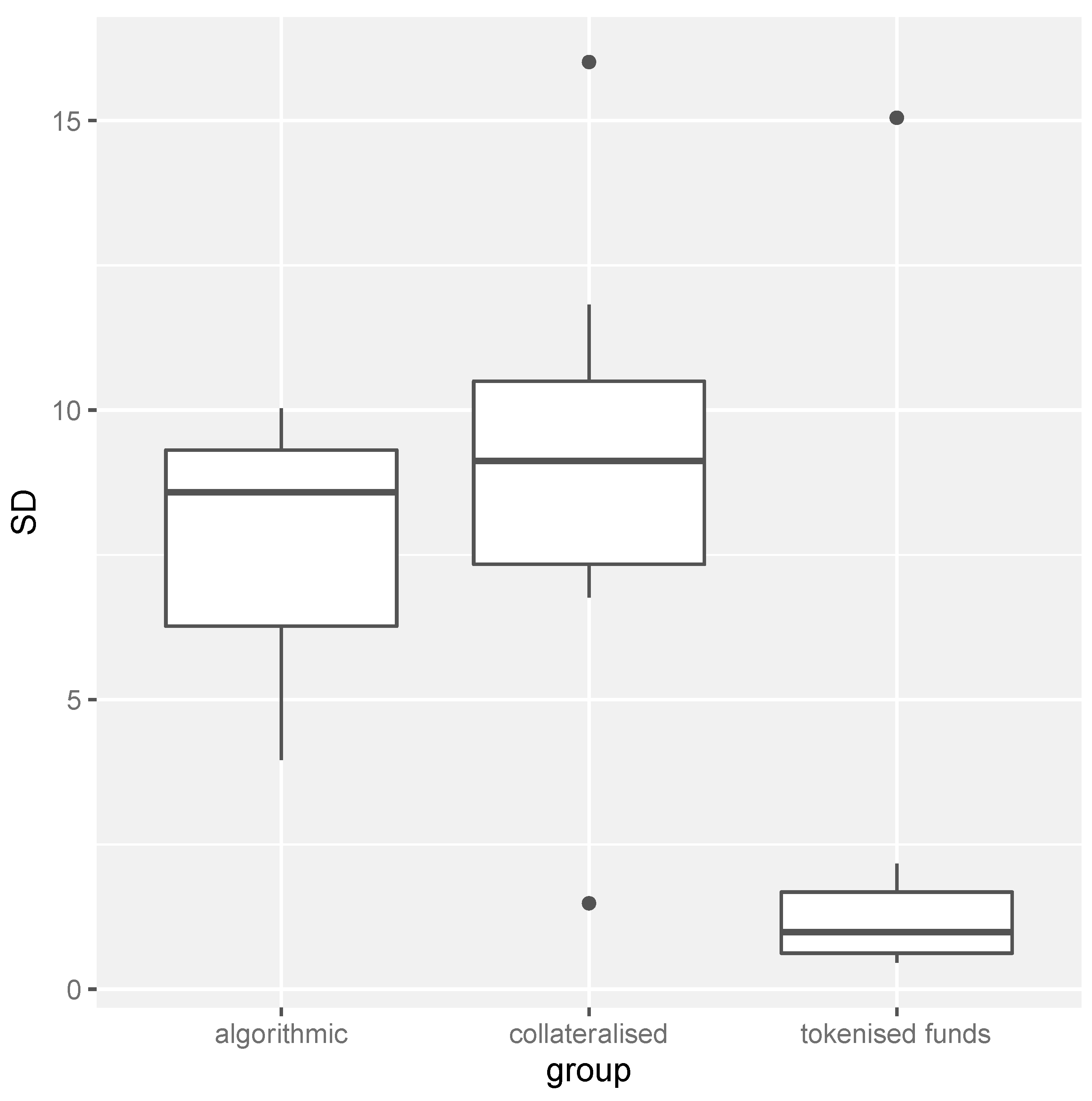
The boxplot below (Figure 2) presents an SD of daily returns for three groups of stablecoins, i.e., tokenised funds, collateralised stablecoins and algorithmic stablecoins.

A quick visual analysis of the boxplot above suggests that the volatility of tokenised funds is lower compared to other groups of stablecoins. Still, the results have to be confirmed by a formal analysis.

The results of testing for normality of residuals and homogeneity of variances suggest that the assumptions of ANOVA are not met. Although there is no reason to claim that variances are not homogenous, one cannot assume normality of residuals (cf.

Table 2. Results of tests for normality of residuals and homogeneity of variances.

Null Hypothesis	Normality of Residuals		Homogeneity of Variances
Test	Shapiro–Wilk Normality Test	Kolmogorov–Smirnov Test	Bartlett Test	Fligner–Killeen Test	Levene Test
Value of the test statistic	0.8619	0.45004	0.64207	2.2536	0.0965
df	-	-	2	2	2
p-value	0.008491	0.000324	0.7254	0.3241	0.9085

Source: authors’ own calculations based on data sourced from coinmarketcap.com.

).

Therefore, the nonparametric procedure of the Kruskal–Wallis test was utilised and confirmed with the nonparametric bootstrap F-test for comparing more than two independent means. The results of both the tests are presented in

Table 3. Results of Kruskal-Wallis test and bootstrap F-test.

Test	Kruskal–Wallis Test	Bootstrap F-Test
Value of the test statistic	7.4258 (df = 2)	4.4291
p-value	0.02441 (chi-square)	0.0239

Source: authors’ own calculations based on data sourced from coinmarketcap.com.

.

The 5% (4.9809%) exact critical value for the Kruskal-Wallis H statistic for the sample containing 9-8-3 observations is 5.717460 (the exact critical value for 1% (0.9882%) level of significance is 7.927381 (so the exact p-value is between 1–5%) (Meyer and Seaman 2008).

The result of the Kruskal-Wallis test strongly suggests that at least two groups of stablecoins do not originate from the same distribution when it comes to the analysed measure of volatility. The result of the bootstrap F-test suggests that there is a difference in the mean of the SD of daily returns between at least two groups of stablecoins.

The post-hoc tests performed after obtaining a statistically significant outcome of the Kruskal-Wallis test suggest that there is a significant difference in the distribution of the SD of daily returns between tokenised funds and collateralised stablecoins (cf.

Table 4. Results of nonparametric post-hoc tests.

Test	Tested Groups	Value of the Test Statistic	p-Value
Pairwise Wilcoxon–Mann–Whitney U test with Holm correction	collateralised—algorithmic	-	0.600
	tokenised funds—algorithmic	-	0.170
	tokenised funds—collateralised	-	0.033
Dunn test (p-values adjusted with Benjamini–Hochberg method)	collateralised—algorithmic	−0.3662335	0.714
	tokenised funds—algorithmic	1.5500663	0.182
	tokenised funds—collateralised	2.6621153	0.023

Source: authors’ own calculations based on data sourced from coinmarketcap.com.

).

The results of nonparametric multiple contrast tests are presented in

Table 5. Results of nonparametric multiple contrast tests.

Contrasts *	Estimator	Confidence Interval	Test Statistic	p-Value
[0.5, 0.5, −1]	0.368	(0.003, 0.733)	3.131	0.048
[1, −1, 0]	−0.082	(−0.484, 0.321)	−0.630	0.813
[1, 0, −1]	0.327	(−0.084, 0.737)	2.470	0.110
[0, 1, −1]	0.409	(−0.013, 0.831)	3.006	0.056

* [algorithmic, collateralised, tokenised funds]. Source: authors’ own calculations based on data sourced from coinmarketcap.com.

. The results suggest statistically significant relative effects in two contrasts. Tokenised funds tend to have lower values of SD of daily returns than collateralised stablecoins. What is more, tokenised funds tend to have lower values of SD of daily returns than both collateralised and algorithmic stablecoins.

4. Discussion

The crucial function of all stablecoins is to provide stability in the currency of reference. Thus, the creators of stablecoins employ different mechanisms to achieve this aim. The main objective of our study was to compare the volatility which characterises the main stablecoin design types. We strived to answer the question of whether all stablecoin designs accomplish the goal of minimising their price fluctuations to the same degree. Hence, we employed various non-parametric statistical tests and compared the SD of daily returns. Our study has revealed that various types of stablecoins are not volatile to the same extent.

This result translates into the finding that different stabilisation mechanisms deliver on the promise of providing stability in the currency of reference to varying degrees. From the viewpoint of investors in cryptocurrencies, it means that it does matter which stablecoin they select for their portfolios if stability is what they are looking for.

Specifically, we detected the difference in distribution of the SD of daily returns between tokenised funds and collateralised stablecoins. Taking into account that tokenised funds and collateralised stablecoins account for the majority of the stablecoin market, this result suggests that investors who are looking for stability in stablecoin’s price in the currency of reference should opt for tokenised funds.

The greatest limitation of our study is the inability to rank stablecoin types according to the volatility based on the results. We are not able to create the ranking because we were not able to state statistically significant differences between algorithmic stablecoins and the other types of stablecoins; tokenised funds, in particular. We believe that it was mainly due to a very limited number of representatives of algorithmic stablecoins. This type of stablecoin is relatively new and their designs involve sophisticated algorithms to respond to price changes (cf. Bullmann et al. 2019). Still, the results of nonparametric rank-based multiple contrasts test procedure suggest that tokenised funds tend to have smaller values of SD of daily returns than collateralised and algorithmic stablecoins.

To compare, the study by Bullmann et al. (2019) included only selected representatives of different stablecoin types, i.e., Tether, Dai, and NuBits. They concluded that tokenised funds (Tether) performed better in terms of volatility than the collateralised stablecoin (Dai), while the algorithmic stablecoin (NuBits) showed the highest volatility rates.

The observed phenomena can be explained on a basis of the fact that tokenised funds do not require any kind of adjustment to maintain the peg since they are backed by the currency of reference. In contrast, other stablecoins are either backed by assets which price expressed in the currency of reference change over time (so the volume of assets must be adjusted to price changes to maintain the peg) or they rely on algorithms balancing supply and demand and often require a hight degree of trust in future stablecoin’s successful performance. It appears that none of the existing implementations of other than tokenised funds stabilisation mechanisms work smoothly enough to match the automatic adjustment of tokenised funds.

The difference in the distribution of the SD of daily returns between tokenised funds and collateralised stablecoins and the statistically significant contrast mentioned above is far from providing an optimistic viewpoint on the development of the whole stablecoin market segment because from amongst all stablecoin types, tokenised funds use blockchain decentralisation and smart contracts benefits to the lowest extent. The idea behind tokenised funds relies heavily on trust in the third-party that acts as a custodian for currency reserves. This aspect of tokenised funds’ design resembles the operations of the currency board arrangement. However, under the currency board arrangement, one needs to trust a central bank that it will act according to the arrangement rules and manage to maintain the foreign exchange rate. In turn, the initiators of tokenised funds initiatives, who act as sole issuers of stablecoins, are at the same time privately held entities that operate in the unregulated market of cryptocurrencies. This alone makes the creditworthiness verification a costly and time-consuming process. Thus, tokenised funds do very little to give their investors an opportunity to eliminate the need for a centralised trusted third-party. The price of a stablecoin of this type will be stable in the currency of reference as long as stablecoin holders believe in the issuer’s pledge to repurchase the stablecoin units on demand. In the light of the controversies over the lack of transparent management and audits of reserves (to give one example only, mind the Tether’s case), the tokenised funds functioning model seems to have many imperfections and does not differ so much from the standard trusted third-party model. Therefore, our study also reveals a clear need for improving the existing stablecoin models that already allows for a greater independence from trusted third parties (on-chain collateralised and algorithmic stablecoins) and developing new design models.

The topic of this study can be even further explored. The primary course of action for the future research is to adopt a dynamic approach to the underlying research question. One possibility would be to examine whether the results can be replicated across time, by applying a moving window to the time range. Due to the fact that some of the stablecoins existed for a relatively short time at the moment of the study, we opted not to do that. A longer time series would facilitate that approach. A different possibility involves performing a change point detection analysis. Structural breaks, meaning a change in model parameters brought on by a change in the statistical properties of the data before and after an event, are quite common in financial data. One possible extension to the research is to view our dataset as an unbalanced panel dataset and to look for unknown common breaks (change points) in panel means. Various values of the change should be allowed for each panel at some unknown common time. Antoch et al. (2018) and Peštová and Pešta (2017) developed the techniques suitable for finite T (the number of observations in each panel). Furthermore, their methodologies allow the within-panel dependent errors to follow AR or GARCH processes. Thus, the approach laid by Antoch et al. (2018) and Peštová and Pešta (2017) would be advantageous in our case. Other avenues for future research include focusing on a risk management point of view of our findings. The groundwork for that has been established in the works by Wang et al. (2020) and Baur and Hoang (n.d.).

5. Conclusions

Our study is the first one ever to measure statistical differences between the average volatility that characterises the main stablecoin design types in order to answer the question of whether all stablecoin designs accomplish the goal of minimising their price fluctuations to the same degree. We opted for a static volatility measure, i.e., standard deviation of return rates, corrected it for autocorrelation, and detected differences between distributions of the measure in three stablecoin groups using various non-parametric tests. We proved that stablecoins do not deliver equally on the promise to provide stable market value with tokenised funds being leaders. To scholars, our study furthers the understanding of a relatively new financial innovation, namely stablecoins, and the different ways their designs correlate with their stated goal of stability. To financial market participants, our research underscores the importance of due diligence and caution when choosing to convert assets to stablecoins due to significantly different volatilities of various stablecoins. Nevertheless, a further academic inquiry into the different aspects of stablecoins is still needed.