Article

The Evolution of Arrears among US Households 1995–2013

College of Business, Arts and Social Sciences, Brunel University London, London, Uxbridge UB8 3PH, UK
J. Risk Financial Manag. 2021, 14(2), 43; https://doi.org/10.3390/jrfm14020043
Submission received: 13 November 2020 / Revised: 5 January 2021 / Accepted: 13 January 2021 / Published: 20 January 2021
(This article belongs to the Special Issue Household Finance)

Abstract

:
This paper looks at arrears among US households between 1995 and 2013. It uses household data from the Survey of Consumer Finances (SCF) where arrears occur when a household reports it “sometimes got behind or missed a payment”. The key contribution is that it decomposes the change in arrears into a behavioural part and a compositional part. Older poorer households increased arrears between 1995 and 2001 (this reversed in 2004). Younger middle-income households increased arrears in 2004. Following bankruptcy reform, wealthier households under 50 reduced their arrears between 2004 and 2007. During the sub-prime recession, everyone except younger low income households increased their arrears. The decomposition exercise shows that most of the changes over time are attributed to changes in arrears once the loan is given and not to the change in the composition of the pool of borrowers.
JEL Classification:
D12; D14; K42

1. Introduction

This paper investigates the changing pattern of arrears among US households from 1995 to 2013. It will explore who enters arrears and how arrears have changed over time for different sub-groups of the population. The key contribution of the paper is to decompose these changes into a contribution from changes in application behaviour, a contribution from changes in acceptance behaviour by lenders, and a contribution from changes in the behaviour of borrowers; as well as a contribution from changes in the characteristics of households. Although a descriptive approach, rather than deriving behaviour from an underlying theoretical model, this decomposition exercise is fundamental to the policy debate, but has never been undertaken before this study.
Between 1995 and 2013, the US suffered two recessions. The first lasted from March to November 2001, and coincided with the dot-com crisis. The second one, lasting from December 2007 to June 2009 (the official NBER dates), was more serious: precipitated by the sub-prime crisis, it is often attributed to lax lending standards in the years immediately before. From the 1990s, there was a sustained increase in the rate of bankruptcy filings by US households (White (2007), showed it quintupled between 1980 and 2004). This motivated the Bankruptcy Abuse Prevention and Consumer Protection Act of 2005, which made bankruptcy, and by implication default, more onerous. This paper will investigate how these three events affected household repayment behaviour by using data from the Survey of Consumer Finances; a survey of US households conducted every three years. The data show that household arrears increased steadily up until around 2005, fell sharply following the passing of the Bankruptcy Act in 2005, before increasing again during the sub-prime crisis (this pattern closely follows the national bankruptcy filing rate). This paper will document the changes in arrears, investigating which households entered arrears and how this changed over time. It will also investigate how borrowers and lenders responded to these events.
There is already a large range of literature, extensively reviewed in Section 2, on household arrears and default for the period studied in this paper. Much of the literature on the behaviour of US households has argued that there was a change in the lending behaviour, as lending standards became more lax. Other papers have argued that there has been an increase in the willingness of households, especially lower income households, to take on more debt. This paper can shed light on these arguments through the following decomposition exercise. For a household to enter arrears, it must first request a loan; it must have the credit application accepted; and it must fail to repay when the loan is scheduled for repayment. Changes in arrears can result from changes in any of these three factors: an important and unique contribution of this paper is that it provides estimates of the size of each factor (and of the size of the effect of changing household characteristics on arrears). Studies which only estimate an overall probability of arrears can provide little insight into why the arrears (or default) have changed over time. For example, much of the policy debate following the sub-prime crisis has aimed to address the perceived lax lending standards of banks prior to the crisis; however, this presumes that the increase in arrears is caused by previously refused households being given credit, rather than a change among households already given credit. However, the results will show that most of the changes in arrears are driven by changes in borrower behaviour, rather than changes in applications or acceptances. This is rather surprising, and suggests that explanations of the changes in the level of household default should concentrate on explaining these swings in borrower behaviour rather than on changes in the composition of the borrower population.
The rest of the paper is organized as follows. The existing literature on household default is surveyed in Section 2. Section 3 describes the data and Section 4 describes the decomposition and the estimation method. The paper will report some preliminary parametric results in Section 5. However, the preferred results arise from non-parametric estimates that fully capture the non-linear effect of income and age (and their interaction). The conclusions are drawn in Section 6.

2. Literature Review

There are a large number of previous studies which investigate default by households for part or all of the period between 1995 and 2013. For example, Berkowitz and Hynes (1999); Domowitz and Sartain (1999); Fay et al. (2002) use survey data to investigate the determinants of bankruptcy filings among US households. Much of the more recent research has tried to assess the causes of the sub-prime recession. Many studies looked at mortgage loan data and at county or post-code area: Mian and Sufi (2009) investigate mortgage defaults using data provided by Equifax at the level of the ZIP code for 1990–2008 and argued for the importance of “declining underwriting standards as a contributory factor in the subprime crisis”. Others, such as Dick and Lehnart (2010), have looked at data on individual loans, and argue that deregulation led to an increase in the supply of credit in the 1980s and 1990s. Demyanyk and Hemert (2011) and Mayer et al. (2009) use information contained in lender records from LoanPerformance to show that (after controlling for observable characteristics) mortgage delinquency increased in the years immediate prior to the sub-prime crisis, and both argued that deteriorating lending standards or loan quality appears to be the main culprit in explaining this rise. Foote et al. (2009) use the same data to show how falls in income drive default. Elul et al. (2010) combine LPS and Equifax data to explain mortgage arrears during the crisis, again concentrating on the population of mortgagors. However, looking at actual borrowers ignores the lenders’ decision to give credit. Dell’Arricia et al. (2012) include rejected loan applicants in their sample, and argue that there was an increase in credit demand. In contrast, Gerardi et al. (2013) use the PSID, arguing that unemployment and negative equity are prime explanations for default.
There is also substantial literature on the effect of the 2005 Bankruptcy Reform Act. The Act attempted to address the dramatic increase in the rate of bankruptcy filings by households in the years leading up to the reform (see White (2007) for a thorough overview of the reform). Prior to the reform, households could file for bankruptcy under Chapter 7 (in which all debts are expunged in return for the surrender of all non-exempt assets) or under Chapter 13 (whereby households proposed a repayment plan but kept their assets). Since households could choose under which chapter to file, the Chapter 7 exemptions set the maximum amount that debtors could be made to pay when filing for bankruptcy, and these exemptions could be very generous: several states allowed an unlimited homestead exemption. The 2005 reforms subjected Chapter 7 filings to an income test; reduced the ability of households to claim the homestead exemption; and raised the cost of filing, partly by subjecting filers to mandatory counselling and financial management courses.
These reforms changed households incentives to default; they also made it more difficult for households to default on credit card debt but continue to repay their mortgage (as had been common under Chapter 7). Livshits et al. (2010) note that prior to the reform, ‘the rise in filings appears mainly to reflect changes in the credit market environment’. White (2007) argues ‘the increase in credit card debt...provides the most convincing [reason for the] increase in bankruptcy filings’, and the reforms encouraged the expansion of credit card debt by lenders, as it became easier to recover these debts. Using state level data, Morgan, Inverson and Botsch Morgan et al. (2012) argue that after 2005, there was an increase in mortgage foreclosure and a reduction in delinquency on personal loans in high exemption states. Li et al. (2011) use data on individual mortgages to argue that default rates increased, particularly among those affected by the means test introduced by the reforms. In a calibration exercise, Athreya et al. (2015) simulate the US economy in which heterogeneous agents face labour market and unemployment risks to investigate the role of the 2005 bankruptcy reform on delinquency and bankruptcy filings. They argue that reform reduces the demand for credit but increases the supply and that the reform would have reduced delinquency but for the sub-prime recession.
Much of the literature above on the sub-prime recession has looked a mortgage debt; in contrast this paper will concentrate on all debts. While mortgage debts are typically larger, most default is associated with concurrent delinquency on non-housing debt. For example, Elul et al. (2010) argue that mortgage defaults are associated with high credit card utilization rates and negative equity, with especially serious default rates when these factors both occur at the same time. Gerardi et al. (2013), using the PSID, note that households in serious arrears invariably have large levels of outstanding unsecured debt.
Changes in arrears can be attributed to changes in the incidence of households applying for loans; changes in the rate at which loans are accepted; or changes in the rate at which borrowers repay their loans. In the review of the literature above, several papers noted an increase in the supply of credit while Athreya et al. (2015) argues for a reduction in credit applications. Keyes et al. (2010) argue that securitization has had a negative effect on the screening incentives of sub-prime lenders, suggesting an increase acceptance rate. An alternative view, expressed in Guiso, Sapienza and Zingales Guiso et al. (2013), is that there was an increase in households’ willingness to default, given their circumstances, during the recession. This paper will discuss the relative importance of changes in applications, acceptances, and arrears among borrowers in the changing arrears behaviour of American households.

3. Data

This paper uses data from the Survey of Consumer Finances (SCF). This survey, conducted by the US Federal Reserve Board normally every three years, is designed to give detailed information on the income and assets of US households, as well as information on the demographic characteristics of each household in the survey. More complete details on the survey design are contained in Kennickell (2012) and Bricker et al. (2014). As well as income and assets, the SCF also records information on households’ borrowing behaviour: in particular, households report whether they have applied for credit (and whether their application was accepted); whether they currently have a loan, and whether they have made each scheduled repayment on time. However, the survey does not report details of the lender, and hence cannot offer much insight into the behaviour of banks. Nevertheless, the paper will exploit this information about US households to understand the evolution of repayment behaviour over the last 20 years. (One problem is that information on applications, including refusals, relates to the last five years, but information on loans and their repayment pertain to the last year only).
This paper concentrates on households aged between 25 and 65 (older and younger households are excluded). Since the primary focus of the analysis is households who use borrowing to smooth consumption, we exclude farming and self-employed households from the analysis (as well as households who seem to have no source of income). After this selection, there are around 3500 households in each wave. Income is measured in 2004 real dollars using the all urban consumers CPI index. Since the aim of this paper is to examine what has happened to the repayment behaviour of US households over the last 20 years, it will use questions on loan and repayment behaviour of every wave of the SCF from 1995 to 2013 (the last year for which the survey is available).
Table 1 reports summary statistics (the mean and the standard deviation) for the variables used in the regression analysis, with separate statistics for all households (including non-borrowers), for those who repay their debts on schedule, and those who report arrears. The table shows that nearly two-thirds of households are couples, that over one-third have a university degree, and that over 70 percent of households are white. The table also shows that those households who repay their debts on schedule have slightly higher income than the general population, are more likely to be in a couple, and are more likely to be white. In contrast, those households that report arrears have lower income, are less likely to be in a couple, to have been to university, or to be white.
Of particular interest in this paper is the repayment behaviour of US households. We will therefore look at whether the household responds that they have failed to repay a loan on schedule. Since the survey combines mortgage or other housing loans and non-housing debt when asking households to respond to this question, this paper will too.1 A household is defined as being in arrears if it responds that it “sometimes got behind or missed payments” when asked about the household’s loans. Note that this encompasses widely differing behaviour: it could mean that a household has failed to make a number of payments and has filed for bankruptcy; or it could mean that the household has made a single late payment that they have quickly rectified when they have an otherwise exemplary record. Figure 1 reports the rate of arrears for each year in the sample constructed from the SCF. It also reports the bankruptcy rate for non-business filings in the US.2 Comparing the two series shows that reported arrears in the SCF follows the same pattern as non-business bankruptcy filings, although many more households are in arrears than are filing for bankruptcy. Both series show that arrears and bankruptcy increased steadily in the 1990s, with the recession of 2001 (March–November), associated with the dot-com bubble, having almost no noticeable effect on this trend. Bankruptcy and arrears have fallen sharply after the enactment of the 2005 bankruptcy reforms made bankruptcy more onerous. However, both arrears and bankruptcy have returned nearly to previous levels during the sub-prime crisis, and has only slowly fallen since 2009. The fact that both series show a similar pattern means we can place some confidence in the figures reported by the SCF.
Table 2 reports some further details about borrowing behaviour. The first column looks at the level of default in the sub-population of the SCF included in the analysis (and plotted in Figure 1). It again highlights the steady increase in the rate of arrears in the early part of the sample, the sharp reduction in arrears in the 2007 wave, and the return to high rates of arrears in 2010 and 2013. The second column restricts attention to those actually borrowing; showing a very similar pattern to the first column. Column 3 of Table 2 shows that the proportion of households with a loan steadily increased from 1995 to 2007, before falling back in the last two waves. This immediately highlights that in 2007, there was both an increase in the number of households borrowing and a reduction in the number of households in arrears. Both 2010 and 2013 saw a reduction in the number of households borrowing to levels lower than in 1998, while arrears have risen above the figure in 2007. The table also shows that there was an increase in the rate at which households failed to get the credit they wanted, and a decline in the rate at which households wanted credit. The next section will run regressions to explore the differing behaviour of different household types.

4. Methodology

The raw data suggest that arrears increased among older households in the 2001 and 2010 recessions, but that younger households increased their level of arrears in 2004 and after the crisis in 2008. However, we would like to say something about the underlying causes of the observed changes in arrears behaviour. Suppose we denote
D = 1 l The loan is in arrears C = 1 l The loan application is accepted A = 1 l The loan is applied for
This paper will investigate the incidence of households being in arrears (e.g., whether a household is actually in arrears, rather than the propensity of the household to default on a loan).3 For a household to be observed in arrears, it needs to have applied for credit, to have received the credit it asked for, and then to have failed to repay this credit when it is due. That is, for a household with characteristics X = x in wave t, the probability of observing a household in arrears is
P r t ( D = 1 , C = 1 , A = 1 | X = x ) = P r t ( D = 1 | C = 1 , A = 1 , X = x ) · P r t ( C = 1 | A = 1 , X = x ) · P r t ( A = 1 | X = x )
Hence, a change in the observed arrears behaviour of a household with characteristics X = x could be because of a change in the arrears behaviour of the household if it is given a loan P r t ( D = 1 | C = 1 , A = 1 , X = x ) ; a change in the behaviour of lenders when they receive a credit application P r t ( C = 1 | A = 1 , X = x ) ; or a change in application behaviour P r t ( A = 1 | X = x ) . We can understand the effect of a change in applications between waves t and s by noting
P r t ( D = 1 , C = 1 , A = 1 | X = x ) P r s ( D = 1 , C = 1 , A = 1 | X = x ) = P r t ( D = 1 | C = 1 , A = 1 , X = x ) · P r t ( C = 1 | A = 1 , X = x ) · P r t ( A = 1 | X = x ) P r s ( D = 1 | C = 1 , A = 1 , X = x ) · P r s ( C = 1 | A = 1 , X = x ) · P r s ( A = 1 | X = x )
The change in arrears between waves t and s can be broken down into a part due to a change in applications, a part due to a change in acceptances by the lender, and a part due to changes in arrears among borrowers. Writing
P r t ( D = 1 , C = 1 , A = 1 | X = x ) P r s ( D = 1 , C = 1 , A = 1 | X = x ) = P r t ( D = 1 | C = 1 , A = 1 , X = x ) · P r t ( C = 1 | A = 1 , X = x ) · P r t ( A = 1 | X = x ) P r s ( D = 1 | C = 1 , A = 1 , X = x ) · P r t ( C = 1 | A = 1 , X = x ) · P r t ( A = 1 | X = x ) + P r s ( D = 1 | C = 1 , A = 1 , X = x ) · P r t ( C = 1 | A = 1 , X = x ) · P r t ( A = 1 | X = x ) P r s ( D = 1 | C = 1 , A = 1 , X = x ) · P r s ( C = 1 | A = 1 , X = x ) · P r t ( A = 1 | X = x ) + P r s ( D = 1 | C = 1 , A = 1 , X = x ) · P r s ( C = 1 | A = 1 , X = x ) · P r t ( A = 1 | X = x ) P r s ( D = 1 | C = 1 , A = 1 , X = x ) · P r s ( C = 1 | A = 1 , X = x ) · P r s ( A = 1 | X = x )
shows how this simple decomposition can be constructed. The last part of the right-hand side of the equation has kept the estimates of acceptances among applications and arrears amongst borrowers from time s, but has used the estimate of application behaviour from time t. Hence, this part of the equation captures the effect on arrears of a change in application behaviour. The second part of the equation shows the effect of changing acceptance behaviour on arrears; and the first part of the equation shows the effect of changing the repayment behaviour of borrowers.

Estimation

The estimation strategy entails estimates estimating the probability of a household, with a given set a characteristics, applying for a loan; having the loan application accepted; and repaying the loan when required to do so. These estimates could be constructed as simple Probit regressions, and the analysis will begin by reporting some results that arise from using Probit estimates. However, some more detailed results will be reported using non-parametric estimates.
In the non-parametric estimates, rather than use a fully parametric estimator to describe the effect of a set of household characteristics X i for household i on arrears D i (or applications A i or acceptances C i ), the relationship is estimated using a Kernel estimator which avoids making the strong assumptions that would be necessary if a Probit or Logit estimator is used (see Blundell et al. (2007) for an example of this approach). A clear advantage of using a non-parametric estimator is that it will allow the age-effect, for instance, to differ at different points in the income distribution. It will also allow estimation of highly non-linear (and non-monotonic) effects of the other variables. The kernel estimates of the effect of the household characteristics on arrears E ( D i | X i ) (similarly applications and acceptances) are constructed using the Nadarya–Watson kernel estimator (see Härdle et al. (1988)). The variances of the kernel estimators are constructed using Bowman and Azzalini (1997) (see also Pagan and Ullah (1999)). There will be separate regressions for each wave of the data.

5. Results

Some simple parametric regression results are discussed before the non-parametric results are reported. As we will see, the non-parametric results provide more nuanced details on the results reported in the paper, but are not substantively different from the results arising from the probit regressions. In both cases, the decomposition exercise will find that most of the changes in arrears over time can be attributed to changes in the repayment behaviour of borrowers, rather than changes in either loan applications or loan acceptances.

5.1. Parametric Results

The results from a Probit regression of the effect of a set of household characteristics X i for household i on arrears D i are reported for each wave in Table 3, with similar results across waves. Younger households are more likely to be in arrears than older households (the differences between age-groups is significant in all waves except 2007). Except in the first wave, lower income households are significantly more likely to be in arrears than higher income households. There are also differences in the effect of the other household variables on arrears, but couple, gender, and college education are only significant in one of the waves, and being white is never significant in these regressions.
The supplementary material in the Appendix A reports the results of a Probit regression for wave of the data for the the effect of household characteristics on application behaviour A, acceptance behaviour C and repayment among borrowers R. In each case, the results are broadly in line with expectations. Younger households, and higher income households, are more likely to apply for credit, and more likely to receive credit. Lower income households are less likely to repay should they receive a loan. Most of the other household characteristics do not have a consistent and clear affect on applications, acceptances, or repayment among borrowers.
The results of these individual regressions, in themselves, are of only minor interest. More interesting is to understand how these regression results are changing over time, and how this affects the pattern of arrears in the population over time: understanding this issue is a key aim of this paper. Table 4 reports how overall arrears are changing over time, and the decomposition exercise based on Equation (3) above. The top row of Table 4 reports the predicted level of arrears that arise from the regression results (the weighted average of each households probability of non-payment 
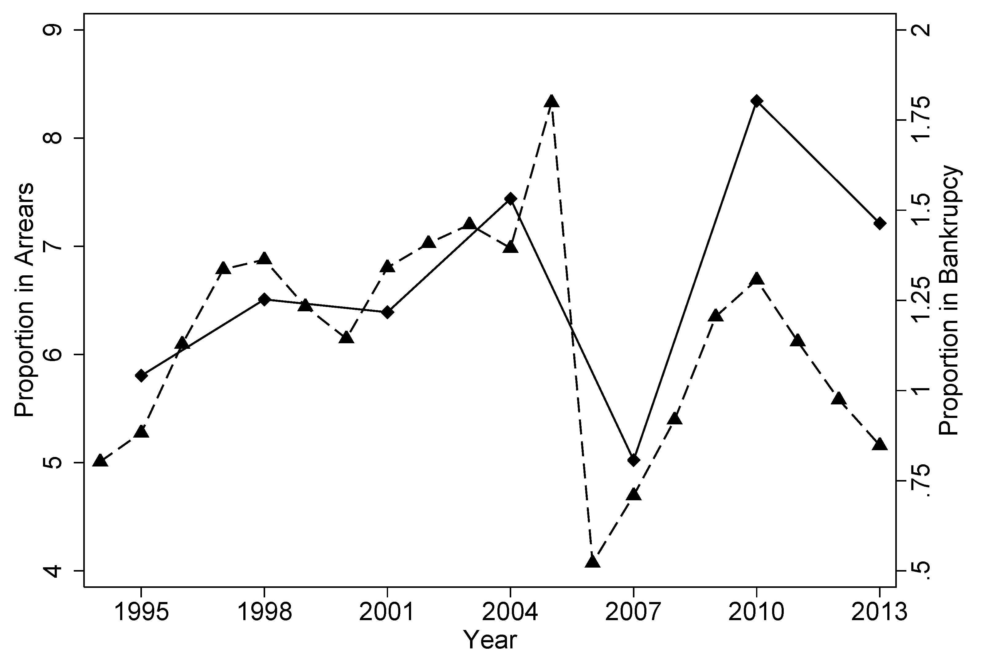
D for each of the waves). It shows that the regression analysis predicts that 6.6 percent of households are in arrears in 1995; this falls to 6 percent in 2001; rises to 8.2 percent in 2004; falls in 2007 (the eve of the financial crisis); and rises again to a peak in 2010. Unsurprisingly, this pattern mirrors the actual arrears in the population reported earlier.
The second column constructs an estimate of the predicted level of arrears in the population using the probit regression coefficients of the current wave P r t , but the characteristics of the households in the next wave X t + 1 .4 Using the 1995 Probit estimates, but the 2001 household characteristics, the predicted level of arrears is 6.27 percent. The 1995 characteristics (the cell above), had predicted a level of arrears of 6.59 percent. This suggests that slightly over half of the difference between predicted arrears in 1995 and predicted arrears in 2001 can be explained by changes in the characteristics of the households between these two waves of the data. What happens when we repeat this analysis for the change in predicted arrears between 2001 and 2004. The table shows that predicted arrears rose 6.04 to 8.22 percent. However, replacing the 2001 household characteristics with the 2004 characteristics only increased arrears to 6.08, a negligible increase. Predicted arrears fall to 6.17 percent in 2007, but the change in characteristics only reduce it to 7.94; again, a very small effect. In the last wave, the regression model predicts arrears at 8.85 percent, but the change in characteristics between 2007 and 2010 only increases arrears to 6.46 percent. The overall story seems to be that changes in household characteristics are only a small part of the explanation of the change in the level of arrears between the different waves of the data.
The bottom three rows of Table 4 show the effect on arrears of first changing the application behaviour of households A, then changing the acceptance of lenders C and finally changing the repayment behaviour of borrowers R. The first column and row three construct the predicted level of arrears using the 1995 household characteristics, the 2001 regression for applications A, and the 1995 regression for acceptance C and repayment R. This means, compared to the top column, the only change is that we are using the estimated application behaviour from 2001 in place of the 1995 application behaviour. This change in application behaviour means that predicted arrears rise from 6.59 percent to 7.00 percent. Arrears fell between these two waves, but the change in application behaviour, by itself, increased arrears. The fourth row shows the effect of using the 2001 regression equation for applications A and acceptances C, which increases arrears to 7.74 percent (again the effect is in the opposite direction to the overall fall in arrears between 1995 and 2001). The last row shows the effect of using the 2001 model for arrears A, acceptances C and repayment among borrowers R, but using the 1995 household characteristics. Predicted arrears fall to 6.41 percent, suggesting a substantial proportion of the change in the overall arrears between 1995 and 2001 can be explained by the change in repayment behaviour of borrowers. The change in arrears between the bottom row of column 1 and the top row of column 2 shows the effect of changing characteristics: arrears fall to 6.04 percent. This suggests there is an important effect from changing characteristics, but this effect is smaller than the change in repayment behaviour.
This type of analysis can be repeated for the changes between the other waves included in the analysis. Between 2001 and 2004, the change in applications slightly increased arrears, and the change in acceptances slightly reduced arrears. However, these effects are small: the largest effect is from the change in repayment behaviour which increases arrears from 6.04 percent to 8.44 percent. Between 2004 and 2007, applications and arrears very slightly increase arrears; but the change in repayment behaviour among borrowers dramatically reduces arrears from 8.51 percent to 6.21 percent. Finally, between 2007 and 2010, the change in application behaviour and acceptance behaviour slightly reduced arrears, from 6.17 percent to 5.98 percent. The change in acceptance behaviour between these two waves then raises arrears to 8.64 percent.
The overall story that clearly arises from the decomposition exercise reported in Table 4 is that the change in default between different waves of the data is that application and acceptance behaviour seem to play little role in explaining the change in arrears (and the sign of their effect on arrears is of the ‘wrong’ sign). There is a moderate effect from changes in characteristics between 1995 and 2001, and again between 2007 and 2010, but the effect is rather small, and cannot explain much of the change in default behaviour. Overwhelmingly, the change in arrears between waves is the result of the substantial swings in the default behaviour of borrowing households.
The change in arrears can differ substantially with household characteristics, and this is investigated in Table 5, although the effect of only some household characteristics are reported.5 It shows that between 1995 and 2001, the oldest age group included in the table had a significant increase in their level of arrears (the changes reported in the table are starred when they are significant at the 5 percent level). However, the other changes between 1995 and 2001 are never statistically significant. Between 2001 and 2004, households between 35 and 44 increase their level of arrears by over 5 percent, and there is a significant increase in arrears for couples and for poorly educated households. Arrears fell between 2004 and 2007 for younger households, and for poorly educated households. The increase in arrears between 2007 and 2010 was significant for middle-aged households and for almost all income groups (although the increase was larger for lower income households). A more thorough investigation of the differences between demographic groups will be undertaken, with some fully non-parametric regressions.

5.2. Non-Parametric Estimates of Arrears

The non-parametric regression results for each of the individual waves are reported in detail in the supporting material in Appendix B, and are only summarised here since the main focus of the paper is the decomposition exercise. Each regression includes age and income, and some households characteristics as explanatory variables, with separate regressions estimated for each wave of the SCF. The main section of the paper will plot the results using figures; they are discussed further in the appendix. The figures do not plot confidence intervals, since it would make the figures too cluttered to be easily read. The analysis here will also concentrate on the age and income variables although other household characteristics are included in the kernel regressions. The non-parametric results will confirm that most of the changes in arrears over time can be attributed to changes in the repayment behaviour of borrowers rather than changes in either loan applications or loan acceptances.
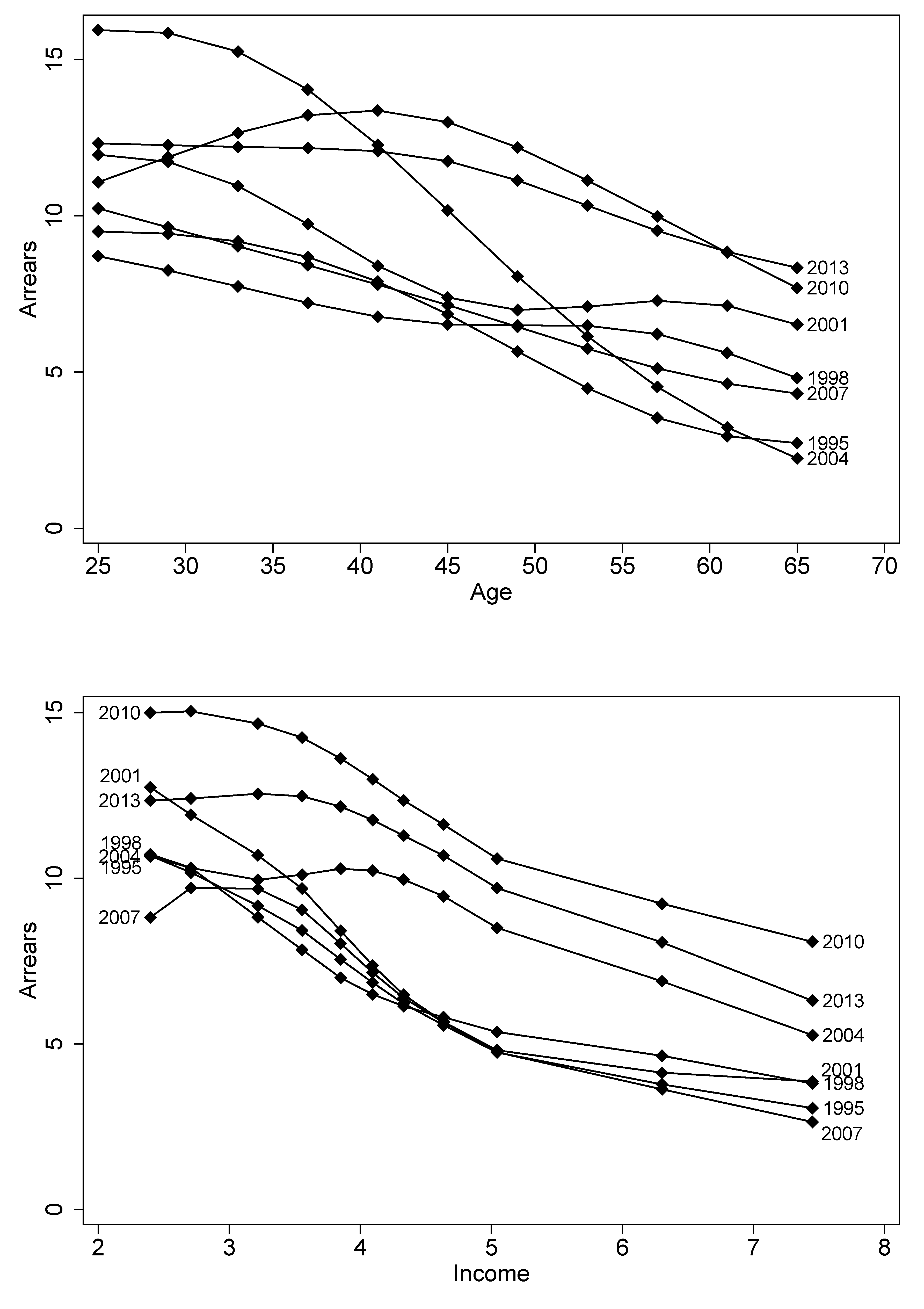
Figure 2 plots the regression results for the level of arrears among all households for each wave of the data from 1995 to 2013 (Appendix B contains more details). The top panel shows how the age profile of arrears has changed for each wave of the survey (holding the other variables at their median value). Arrears are two-to-three times higher at younger ages than at older ages; and the difference between age groups is statistically significant in every wave. Middle-aged households have intermediate rates of arrears.
More interestingly for this paper, arrears for each age-group change from year to year. By 2001 (the year of the dot-com crisis), the arrears rate is significantly higher than in 1995 for households aged 53 and above: at age 65, the rate of arrears increased from 2.72% of households to 6.52% of households. In 2004, the youngest households under 45 are significantly more likely to report arrears compared to 1998 or 1995. However, older households are not now more likely to enter arrears than in these earlier years (repayment rates are significantly higher among households age 57 and over in 2004 than in 2001).6 Recall that households were surveyed in 2007 before the sub-prime crisis had started, but after the Bankruptcy Reform Act of 2005 had tried to make bankruptcy more difficult for those with above median levels of income.7 The rates of arrears among younger households recovered in 2007 (their arrears was significantly lower than in 2004), but arrears for older households are not significantly different to earlier years. The contrast between the 2010 and 2007 wave reflects the effect of the subprime crisis. The figure shows arrears increased significantly at all age-groups over the age of 35, and these rates of arrears remained high in 2013. The preliminary conclusion from this analysis is that arrears increased among middle-aged and older households both in the dot-com recession and in the subprime crisis, and that arrears among younger households had been especially high just prior to the Bankruptcy Reform Act of 2005.
The effect of income on arrears at age 45 is reported in the bottom panel of Figure 2. The figure plots arrears for each decile of the income distribution (and at the 5th and 95th centile). In 1995, over 10% of households at the 5th centile of income (the bottom of the income range) are in arrears, but only 3% of households at the 95th centile are in arrears. The results in 1998 and 2001 show similar differences by income (these differences are statistically significant). In 2004, there has been a sharp, statistically significant increase in arrears, especially among middle-income and higher income households. The fact that the increase in arrears was among these income groups explains the focus that the Bankruptcy Reform Act of 2005 placed on making it more difficult for richer households to escape their debts. Indeed, in 2007, there was a statistically significant fall in rates of arrears among middle and higher income households: rates of arrears had returned to those observed in earlier years, suggesting that the Act had succeeded in its objectives. Arrears increased following the onset of the subprime crisis in 2010: low, middle, and high income households all increased arrears by around 6%. In 2013, there was a small but statistically insignificant recovery in rates of arrears at all income groups.
A key advantage of using a non-parametric estimator is that the estimation can allow for the effect of income to be different for younger households compared to older households. These results are discussed in more detail in the supporting evidence. For households at age 30, over 13% of households at the 10th centile of income are in arrears in 1995, while only around 4.4% of households in the 90th centile are in arrears. In contrast, for 60-year-old households, 5.2% households at the 10th centile of income are in arrears, while being only 1.6% of the 90th centile rate of arrears. These differences are statistically significant. These arrears changed over time. By 2001, there was a sharp deterioration in repayment rates for lower income households, with poor older households more likely to be in arrears than poor younger households: at the 10th income decile, the rate of arrears is around 15.1% for 60-year-olds, but only 11.9% at age 30. In 2004, with the recovery of the economy after the dot-com recession, the rate of arrears of low-income older households recovered to pre-recession levels, and, surprisingly, differences across income levels for these older households are no longer statistically significant. In contrast, younger household arrears increased at all income levels (these differences are statistically significant for middle-income households). Rates of arrears for the youngest households fell in 2007: from 14.7% to 10.4% for households at the 10th income centile; from 15.7% to 9.6% for middle-income households; and from 9.6% to 5.2% at the 90th centile. Older households, however, have not significantly changed their level of arrears. Overall, young and middle-aged households of middling income increased their rate of arrears in 2004, and that the Bankruptcy Reform Act of 2005 was successful in reversing this increase in arrears in 2007. Following the sub-prime crisis, for younger households, arrears increased for all income groups: low-income households increased arrears from 10.3% to 15.2% (although this is not statistically significant); while high income household arrears increased from 5.2% to 9.8%. Arrears also increased for older households: lower income households increased arrears from 5.6% to 11.9%, while higher income households increased arrears from 2.3% to 5.1%. These results are similar to what we found for middle-aged households.

5.3. Application and Acceptance Behaviour

A key aim of the paper is to understand the extent to which the changing pattern of arrears can be attributed to either changes in the application behaviour of households or the lending behaviour of banks. Section 5.4 below will describe this decomposition, but before proceeding, it is necessary to briefly describe some estimates of the probability of a household applying for a loan and the probability of an applicant household receiving a loan (these results are described in more detail in the additional supporting material in Appendix C at the end of the paper).
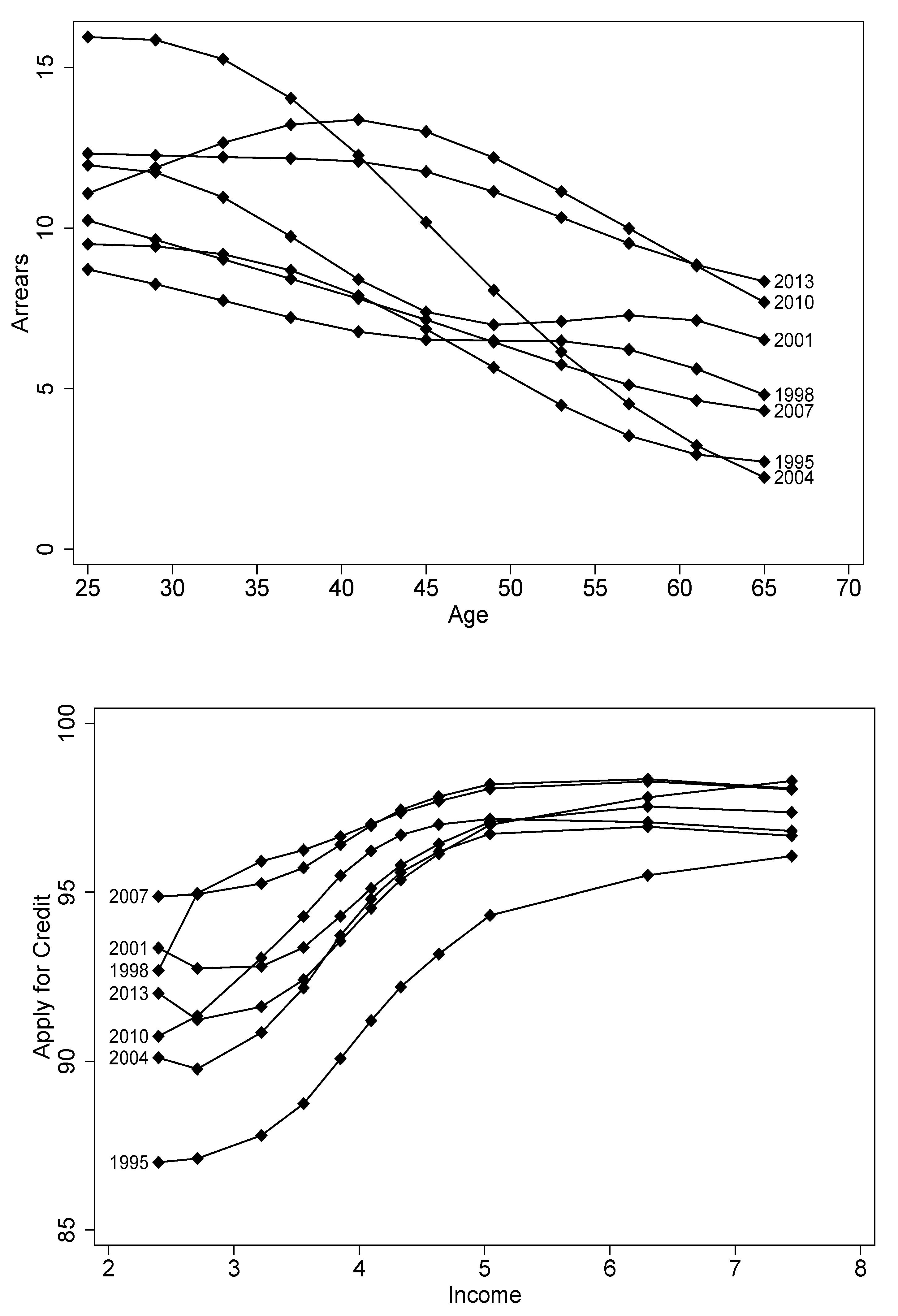
Figure 3 shows how application behaviour has been changing between waves: the top panel shows application behaviour at different ages, while the bottom panel shows different income groups in each wave; in each case, all other variables are held at their median. The top panel shows that, while in each year, the difference across age groups is not large, nevertheless, credit applications have been changing over time. Significantly more households desired credit in 1998 than in 1995 at all age levels (there was a 3 percent increase at younger ages, and a 4 percent increase at older ages). Similarly, in 2007, the demand for credit was significantly higher than in 2004. The demand for credit then fell significantly in 2010 for the oldest households, and had fallen back to 2004 levels for all households by 2013.
The bottom panel of Figure 3 shows that in each year, low income households are significantly less likely to apply for credit than high income households. Moreover, the proportion of households wanting credit in each income group has been changing over time. More households wanted credit in 1998 and 2001 compared to 1995, and this increase was larger for lower income households. There was a small, but statistically insignificant decline in the desire for credit in 2004, before the desire for credit recovered in 2007: this increase was concentrated in lower income households. Finally, there has been a decline in households reporting that they would like a loan between 2007 and 2013.
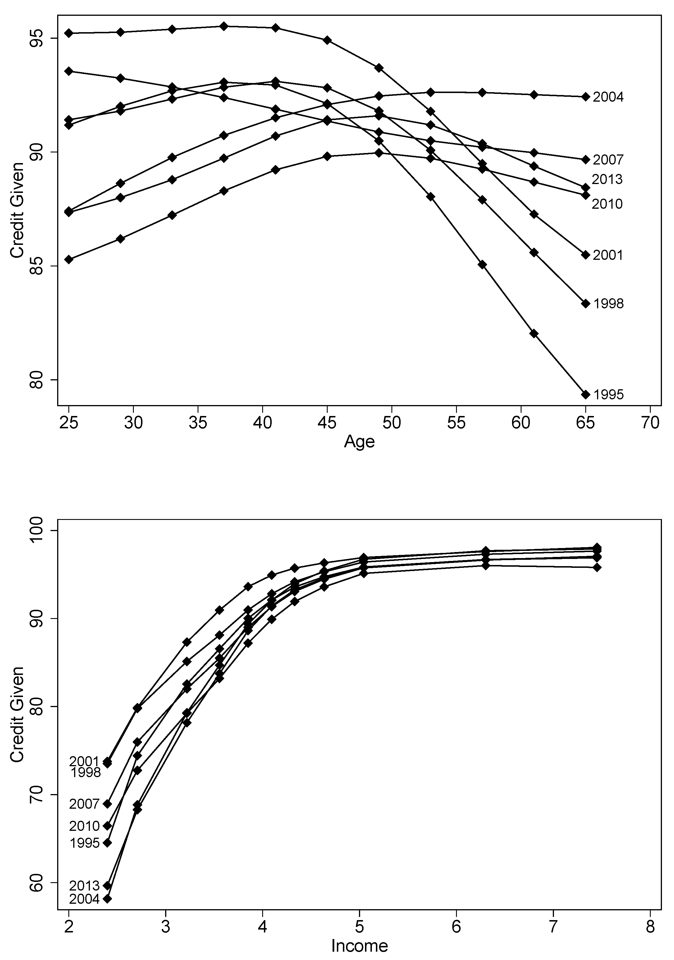
Figure 4 describes the rate at which credit applications are accepted by the lender and given the loan. The top panel of the figure shows that in the early years of the sample; younger households are significantly more likely to get the credit they want than older households. Although credit acceptance increased for all households in 1998 and 2001, this increase was larger for these older households. In 2004, credit to older households continued to increase, while there was a sharp decline in credit to the youngest households. This decline reversed in 2007. In 2010 and 2013, households of all ages saw a decline in credit acceptance, but the falls are largest (and only statistically significant) for the youngest households.
The bottom panel of Figure 4 shows that, in all years, low income households are significantly less likely to get credit they want than high-income households. At the top of the income distribution, there is no statistical difference in credit acceptance over the years, as changes in credit acceptance over time are concentrated in middle- and low-income households. For example, middle-income households are 2.8 percent more likely to get credit in 2001 than in 1995, while households at the 10th income centile are 5.4 percent more likely to get credit in 2001 (although the higher variance of the low-income estimates mean this difference in not statistically significant). Credit acceptance declined in 2004 for all households below the 50th centile, with the declines much larger for the lowest income households, and failed to much recover in 2007. The results in 2010 and 2013 are similar to those in 2004.

5.4. Decomposing the Arrears Behaviour

The raw data suggest that arrears increased among older households in the 2001 and 2010 recessions, but that younger households increased their level of arrears in 2004 and after the crisis in 2008. However, we would like to say something more about the the observed changes in arrears behaviour. Table 6 shows the results of the decomposition exercise described by Equation (3) in Section 4. It reports the change in default for 1995–2001, 2001–2004, 2004–2007 and 2007–2010 in bold, with the results starred when the regression results reported earlier had shown the changes to be statistically significant at the 5 percent level. For age and income, these results correspond to those reported in Figure 2. Looking at the table, the first result in bold at the top of the left-hand column shows that for 25-year-old households, arrears increased by 2.63 percent; but this is not statistically significant (it is not starred). The next three columns denote how much of the change in default can be attributed to changes in applications (A), to credit acceptance among applicants (C), and to repayment among borrowers (R) using Equation (1) above. The effect of changes in application behaviour (holding acceptances and arrears among borrowers fixed at their 1995 level) is to increase arrears by 0.26 percent; the effect of credit-acceptance increases arrears by 0.40 percent and repayment among borrowers increases arrears by 1.98 percent between 1995 and 2001. Overall, putting all these effects together results in a increase in arrears behaviour, which, however, is not statistically significant. We can repeat this process for each group and each pair of years in the table to review the cause of the observed changes in arrears behaviour, in order to better understand what has happened during the period of study.
Between 1995 and 2001, the change in arrears was found to be significant for households whose head is age 53 and over (the change in arrears, shown in the bolded Δ D column, is marked with an asterisk). At 53, the arrears increased by 2.71 percent. The decomposition exercise shows that the change in application behaviour (shown in column A), increased arrears by 0.17 percent; the change in acceptance behaviour (column C) increased arrears by 0.18 percent; and the change in the repayment behaviour of borrowers (column R) increased arrears by 2.35 percent. This result suggests that over 85 percent of the change in arrears among 53-year-old households is driven by changes in borrower behaviour rather than changes in the composition of the borrower population. A similar conclusion arises for households aged 57, where changes in repayment among borrowers account for 3.45 percent of the 3.75 percent change in arrears; and the results are also similar among 61-year-old households and 65-year-old households where most of the change in arrears again seems to be the consequence of a change in the repayment behaviour of borrowers.
Table 6 shows that between 2001 and 2004, 29-year-old households increased arrears by 3.76 percent, and that this change was earlier found to be statistically significant at the 5 percent level. The decomposition exercise shows that changes in application behaviour reduced arrears by 0.12 percent and that changes in acceptance by lenders reduced arrears by 0.77 percent. The main cause of the increase in arrears for 29-year-old households was that there was an increase in arrears among borrowers (the decomposition exercise shows this would have increased arrears by 4.66 percent). The results for households aged between 33 and 45 had earlier all shown significant increases in arrears (they all starred in the table). In all cases, the decomposition exercise shows that this increase in arrears was despite a reduction in applications (the effect of applications A is negative in each case) and a reduction in lending to these households (column C shows the effect of acceptance is also negative). The increase in arrears among these households is driven by a change in the repayment behaviour of borrowers, shown in column R. While younger households increased arrears, there was a significant reduction in arrears among older households over 60. The decomposition exercise shows that, while the change in applications has the right sign, the effect on arrears is tiny. Changes in acceptance behaviour have the wrong sign: it increases arrears by 0.40 percent among 61-year-old households, and by 0.50 percent among 65-year-old households. The exercise shows that the reduction in arrears for households over 60 is overwhelmingly because of changes in the behaviour of households who receive a loan, as shown in column R. Low education households also had a significant increase in arrears between 2001 and 2004, and the decomposition attributes this increase to a change in borrower behaviour, rather than to a change in either applications or acceptances.
Between 2004 and 2007, 45-year-old households and younger significantly decreased arrears while for older households there is a statistically insignificant increase in arrears. Again, these changes are almost entirely due to changes in non-payment among borrowers (column R), since there were negligible effects on arrears from changes in the demand for loans (column A) or in credit acceptance (column C). Couples and non-college-educated households also significantly reduced their arrears (column D), and the decomposition exercise shows that the change can be overwhelmingly attributed to changes in arrears among borrowers (column R).
In 2010, there was an increase in arrears among all households except those under 30, with the largest increase among middle-aged households. As before, the increase can be attributed to changes in arrears behaviour among borrowers (the changes in wanting a loan, or being denied credit, by themselves, contribute to a very small reduction in arrears as the sign of the effect is negative in column A and column C). Younger households have a smaller increase in arrears, which would have been much larger if there had not been an increase in credit refusals, shown in column C. However, if demand and credit acceptance had not changed, the increase in arrears would still have been smaller than for middle-aged or older households (see column R). This suggests that the reduction in credit may not have been aimed at those age-groups, which increased arrears the most. Couples and non-college households also had a large increase in arrears between 2007 and 2010 (over 5 percent in each case). In both cases, applications and acceptances had the effect of slightly reducing arrears, but there was a very large change in borrower behaviour, which caused an overall increase in arrears for these groups.
The results so far suggest that behaviour differs for young and old households (other variables held at their median). The second half of the table looks at the income distribution at age 30, age 45 and age 60. It shows that the change in the rate of arrears for young and middle aged households between 1995 and 2001 is never significant. However, for old households, the changes are large, positive, and significant for all households at or below the 70th income centile (these results are starred in the table), and the increase is larger for lower income households. This increase is mostly attributable to changes in the behaviour of borrowers (column R), with much smaller changes attributable to changes in application behaviour (column A) or lending behaviour (column C). For example, at age 60, applications increase arrears by 0.44 percent for households at the 10th income centile, while more generous lending increases their arrears by 0.69 percent. However, the reduction in repayment among borrowers increases their arrears by 8.80 percent, which is a much larger effect.
What about the changes between 2001 and 2004, during which the economy recovered from the dotcom crisis? This period is just prior to the bankruptcy reforms enacted in 2005; recall that Figure 1 shows a sharp spike in bankruptcy filings in 2005. The results shown in Table 6 show that for 60-year-old households, there was a significant reduction in arrears for households below the 60th income centile. The decomposition exercise shows that this reduction in arrears among older households is almost entirely attributable to a reduction in arrears among borrowers (column R): changes in applications had a very small effect, while column C shows that there was a reduction in lending to the lowest income households (which reduced arrears by 2.26 percent for households at the 5th centile), but that lending actually became more generous for households at or above the 20th income centile. It seems that, for older households, the decrease in arrears fully reversed the earlier increase between 1995 and 2001, and moreover, these changes are mostly attributable to changes in the repayment behaviour of borrowers. However, for middle-aged households, there was a statistically significant increase in arrears for households between the 50th and 90th income centiles, while for the youngest households, arrears increased for households between the 50th and 70th income centiles. For these middle-aged and younger households, column A shows a very small reduction in applications, while column C shows a small reduction in lending, hence neither can explain the increase in arrears. Rather, column R shows that the increase in arrears is explained by the worsening repayment behaviour of households receiving a loan.
After the enactment of the bankruptcy reforms in 2005, Figure 1 shows a sharp reduction in bankruptcy filings in 2006 and 2007. However, our results show that the change in arrears between 2004 and 2007 is never significant for older households (and the point estimates of the change are small). The reduction in arrears was instead concentrated on younger households between the 30th and 90th income centiles, and on middle-aged households between the 50th and 90th income centiles. Perhaps surprisingly, these are mostly the households which had increased arrears between 2001 and 2004. For younger households between 2004 and 2007, the decomposition exercise shows that the reduction in arrears is not due to changes in either application or lending behaviour (column A shows that applications are increasing arrears, while column C shows that lenders became more generous in giving loans to younger households). For middle-aged households, an increase in applications again had the effect of slightly increasing arrears, while there was a negligible reduction in arrears resulting from changes in lender behaviour. Column R shows that the overall change in arrears between 2004 and 2007 can be attributed to changes in the repayment behaviour of borrowers. Given that an aim of the bankruptcy reform of 2005 was to encourage higher income households to repay their debts, it seems that the reforms succeeded in their aim among middle-aged and younger households. Moreover, the reforms had remarkably little effect on lender behaviour.
The rate of arrears shown in Figure 1 sharply increased in 2010. This increase has often been attributed to lower income households receiving credit hitherto refused, and consequently defaulting on their debts (hence the sub-prime crisis). The regression results reported earlier also show that between 2007 and 2010, there was a significant increase in arrears across all income groups for middle-aged and older households, and for households above the 70th income centile among younger households (this is shown by starring the change in arrears in Table 6). The size of the change among 60-year-old households was larger for lower income households than higher income households; but there were rather smaller differences across income groups among 45-year-old households. The decomposition exercise shows that applications and acceptances (columns A and C) had a negligible effect on arrears (and the sign in both cases is negative). For all income levels, the change in arrears is fully attributable to changes in arrears among borrowers, shown in column R. Table 6 shows that the change in arrears between 2007 and 2010 for young lower-income households is not significant. The decomposition exercise shows that if only the behaviour of borrowers changed, then the overall increase in arrears of these households would have been larger than it was (but still smaller than for higher income 30-year-olds), but that a reduction in the granting of credit roughly halved the change in the rate of arrears for households between the 20th and 40th centile. The increase in arrears does not fully support the story about sub-prime lending driving arrears, for two reasons. First, except among the oldest households, the increase in arrears is not larger among lower income households; in fact, for younger households, it is the wealthier households who have increased their rate of arrears. Second, the decomposition exercise suggests that the increase in arrears can not really be attributed to either increases in applications or acceptances.
The results reported in this section suggest, rather surprisingly, that most of the changes in arrears over time are due to dramatic fluctuations in the repayment behaviour of borrowers rather than to changes in the composition of the borrower population. Studying all three major events (the two recessions and the bankruptcy reform) together has enabled us to see that this feature is common to all three events: the change in the repayment of borrowers explains the increase in arrears of poorer older households between 1995 and 2001 and their reduction in arrears between 2001 and 2004; it explains the increase in arrears of middle-income younger and middle-aged households between 2001 and 2004, and their reduction in arrears in 2007; and it largely explains the increase in arrears for all households (except young low-income households) between 2007 and 2010.

6. Conclusions

This paper has investigated the arrears behaviour of US households between 1995 and 2013, using data on loan and repayment behaviour from the Survey of Consumer Finances. The SCF is a survey of US households, and does not include information regarding the lender, and hence, the study has little to say about the banking sector. Moreover, the analysis of behaviour is not explicitly based on any underlying theoretical behavioural model, but attempts, rather, to describe what the household actually does. The raw data show that arrears increased during the dot-com recession at the beginning of the 21st century, fell in the years immediately following, and then sharply increased during the more recent sub-prime recession. By running fully non-parametric regressions, the analysis is able to explore the differing experiences of different sub-groups of the population. In particular, the non-parametric regressions allow for highly non-linear responses by households, as well as complicated interactions between variables such as age and income. The results show that the increase in arrears in the years leading up to the dot-com recession was concentrated on older households (e.g., households in their fifties and sixties), and especially lower income older households. These older households reduced their arrears between 2001 and 2004, while younger households (especially younger middle-income households) increased their arrears during these years. Between 2004 and 2007, there was a sharp reduction in arrears, but this reduction was concentrated on households aged 45 or younger (especially those at and above average incomes). Lastly, the sharp increase in arrears since the sub-prime crisis has been experienced by all but the youngest lowest income households.
A major contribution of this paper has been to decompose the change in rates of arrears into a contribution from changes in applications, from changes in acceptances, and from changes in repayment among borrowers. Dell’Arricia et al. (2012) and Athreya et al. (2015) have argued that there was a change in application behaviour. In contrast, Mian and Sufi Mian and Sufi (2009), Demyanyk and Van Hemert Demyanyk and Hemert (2011) and Mayer, Pence and Sherland Mayer et al. (2009) emphasise the role of changes in lender behaviour. Perhaps surprisingly, however, the decomposition exercise suggests that most of the changes in arrears between waves are the result of changes in the behaviour of borrowers rather than changes in the composition of the borrower population. Studying the entire span from 1995 to 2013 shows that this feature is consistent across all the major events that affected households during this period (and indeed, this is an important motivation for studying the whole period rather than each major event separately). In both the dot-com recession, and the sub-prime crisis, the increase in arrears is little changed by changes in the application or acceptance rate of those groups who significantly increased their incidence of arrears (preliminary parametric results show that changes in demographics did not play a large role). However, the fact that younger and middle-aged lower income households did not increase their arrears appears to be partly because lenders reduced these households’ access to credit (which seems to have reversed in 2007).
The two most important events during the period studied in this paper are the Bankruptcy Reform of 2005 and the sub-prime crisis at the end of the decade. The bankruptcy reform had the aim of reducing default and non-payment from high income households who could reasonably afford to repay their debts. By comparing changes in arrears among households in 2004 and 2007, this paper has shown that these objectives seem largely to have been achieved. The paper shows that there was little change in either applications or acceptances by lenders between these two years (if anything, poorer households had their access to credit improved). However, there was a sharp and significant reduction in arrears among households over the 30th income centile for 30-year-old households, and among households above median income for 45-year-old households. Perhaps surprisingly, there seems to have been no significant effect on the arrears of older households, even those higher income households which were the target of the reforms.
The second key event affecting US households during the study period is the serious recession resulting from the sub-prime crisis. Much of the literature on mortgage credit argues that changes in acceptances were a key cause of the sub-prime recession, while Livshits et al. (2010) and White (2007) argue that there was a more general increase in credit to households. Athreya et al. (2015) argue that there had been a change in application behaviour. The results reported here, although they include non-housing debts, and do not report the size of the loan, do not seem to support this general conclusion: the decomposition exercise attributes almost all the change in arrears among those groups who significantly increased their rate of arrears to changes in borrower behaviour. Guiso et al. (2013) have argued that there was an increase in households willingness to default, and the results in this paper support their view.
The results reported in this paper have shown that the rate of repayment among borrowers has changed dramatically over the years. However, one might worry that this is being driven by changes in the composition of borrowers. For example, if households hitherto refused credit are given a loan, then these new borrower households might be expected to have much higher default rates than the existing pool of borrowers, causing the average rate of arrears among borrowers to become worse. However, this hypothesis does not seem to explain the changes in arrears during the sample period. For example, between 2004 and 2007, there was an increase in the level of borrowing at the same time as there was a reduction in arrears among borrowers. Similarly, between 2007 and 2010, there was a reduction in both application and acceptances at the same time as an increase in arrears. In both these examples, including or excluding marginal borrowers (who would be expected to have worse rates of repayment) cannot explain the change in the average behaviour of borrower households. The changes between 2001 and 2004 also cannot be explained by these compositional changes, except perhaps for the lowest income older households, since changes in the pool of borrowers has the opposite sign to changes in the arrears of borrowers. While there was a significant increase in arrears among borrowers between 1995 and 2001 for older borrowers, and a concurrent increase in borrowing among these borrowers, the later change was much too small to account for the former change. Hence, the paper concludes that most of the changes in arrears between waves really are driven by changes in borrower behaviour rather than in the composition of the borrowing population.

Funding

This research received no external funding.

Data Availability Statement

The data used in this study, the Survey of Consumer Finances, is available from the Federal Reserve at https://www.federalreserve.gov/econres/scf-previous-surveys.htm.

Conflicts of Interest

The authors declare no conflict of interest.

Appendix A. Additional Supporting Material: Parametric Estimates

The regression results used for the parametric decomposition exercise are presented in the tables below. Table A1 shows the estimates for each wave of the data for repayment among those households who are currently borrowing. It shows that younger households (except in 1995) and lower income households are less likely to repay on schedule, and homeowners, except in 2007, are more likely to repay on schedule. Table A2 reports whether a household has received a loan. It shows that younger households and middle-to-higher income households are more likely to receive a loan, as are homeowners. Table A3 shows whether a household has applied for a loan. The table shows that younger households and middle-to-higher income households are more likely to apply for a loan, as are homeowners. These estimates are used in the paper to describe how the behaviour of households and lenders has been changing over time, and to describe the main contribution of each component of the decomposition exercise in explaining the changes in arrears over time.
Table A1. Probability of Repaying Among Borrowers.
19952001200420072010
Age 25–34−0.196−1.267 **−0.592 **−0.216−0.257
(0.227)(0.406)(0.197)(0.197)(0.144)
Age 35–44−0.146−1.025 *−0.624 **−0.352−0.593 **
(0.228)(0.408)(0.193)(0.193)(0.136)
Age 45–54−0.122−1.154 **−0.300−0.361−0.519 **
(0.231)(0.407)(0.198)(0.191)(0.134)
Age 55–640.167−1.210 **−0.024−0.146−0.274 *
(0.270)(0.411)(0.218)(0.200)(0.140)
Income Decile 1–2−0.897 **−1.440 **−1.531 **−1.862 **−1.133 **
(0.315)(0.366)(0.345)(0.341)(0.159)
Income Decile 3–4−0.715 *−1.325 **−1.346 **−1.695 **−0.885 **
(0.302)(0.356)(0.337)(0.334)(0.151)
Income Decile 5–6−0.602 *−1.091 **−1.299 **−1.368 **−0.626 **
(0.293)(0.352)(0.329)(0.330)(0.148)
Income Decile 7–8−0.329−0.649−0.886 **−1.037 **−0.478 **
(0.300)(0.355)(0.333)(0.329)(0.146)
couple0.148−0.179−0.0060.369 *−0.030
(0.179)(0.162)(0.139)(0.144)(0.104)
gender−0.061−0.020−0.1670.348 *−0.090
(0.171)(0.157)(0.129)(0.140)(0.098)
college0.2470.1640.1410.1370.277 **
(0.133)(0.127)(0.107)(0.116)(0.078)
white0.2110.1890.020−0.0900.085
(0.114)(0.103)(0.093)(0.103)(0.066)
household size−0.110 **−0.058−0.059−0.105 **−0.044
(0.042)(0.039)(0.035)(0.038)(0.026)
homeowner0.575 **0.440 **0.530 **0.1890.197 **
(0.112)(0.105)(0.093)(0.105)(0.071)
Constant1.852 **3.517 **2.945 **2.712 **2.374 **
(0.467)(0.611)(0.458)(0.455)(0.265)
N16802025226525203610
test: Age3.2112.7125.615.5931.78
(prob)0.5230.0130.0000.2320.000
test: Income12.5531.9929.2747.1364.71
(prob)0.0140.0000.0000.0000.000
* p < 0.05; ** p < 0.01.
Table A2. Probability of Borrowing Among Applicants.
19952001200420072010
Age 25–340.634 **0.413 *0.479 **0.535 **0.605 **
(0.151)(0.172)(0.148)(0.157)(0.121)
Age 35–440.545 **0.364 *0.532 **0.431 **0.639 **
(0.149)(0.164)(0.142)(0.145)(0.119)
Age 45–540.430 **0.1750.633 **0.433 **0.404 **
(0.146)(0.154)(0.139)(0.134)(0.105)
Age 55–640.2750.1860.2370.333 **0.254 *
(0.154)(0.162)(0.126)(0.124)(0.102)
Income Decile 1−2−0.381 *0.019−0.133−0.412 *−0.036
(0.182)(0.182)(0.167)(0.162)(0.126)
Income Decile 3–4−0.1050.1950.029−0.0310.035
(0.171)(0.165)(0.152)(0.152)(0.117)
Income Decile 5–60.1380.407 *0.511 **0.2460.435 **
(0.165)(0.160)(0.151)(0.148)(0.118)
Income Decile 7–80.1340.590 **0.269 *0.437 **0.372 **
(0.170)(0.154)(0.131)(0.141)(0.110)
couple0.2130.048−0.273 *−0.0720.142
(0.134)(0.147)(0.132)(0.143)(0.100)
gender0.1520.023−0.024−0.0120.246 *
(0.129)(0.138)(0.127)(0.140)(0.098)
college0.210 *0.046−0.006−0.239 *−0.094
(0.106)(0.112)(0.100)(0.102)(0.077)
white0.186−0.266 *−0.005−0.068−0.059
(0.096)(0.116)(0.097)(0.109)(0.074)
household size0.0540.0190.085 *0.0400.002
(0.037)(0.039)(0.039)(0.040)(0.028)
homeowner0.874 **0.565 **0.721 **0.315 **0.724 **
(0.094)(0.106)(0.103)(0.111)(0.080)
Constant−0.4180.728 *0.4151.086 **0.130
(0.303)(0.345)(0.305)(0.314)(0.228)
N19142176246726763917
test: Age19.387.7224.5315.4235.64
(prob)0.0010.1020.0000.0040.000
test: Income18.7923.3426.6234.1434.76
(prob)0.0010.0000.0000.0000.000
* p < 0.05; ** p < 0.01.
Table A3. Probability of Applying for a Loan.
19952001200420072010
Age 25–341.490 **1.259 **1.053 **0.950 **0.860 **
(0.112)(0.120)(0.117)(0.119)(0.087)
Age 35–441.317 **1.154 **1.069 **0.660 **0.830 **
(0.109)(0.111)(0.112)(0.106)(0.085)
Age 45–541.226 **1.051 **0.865 **0.539 **0.710 **
(0.105)(0.103)(0.099)(0.094)(0.076)
Age 55–640.758 **0.688 **0.559 **0.445 **0.370 **
(0.103)(0.102)(0.093)(0.088)(0.071)
Income Decile 1–2−0.665 **−0.384 **−0.431 **−0.293 *−0.232 *
(0.133)(0.132)(0.127)(0.117)(0.092)
Income Decile 3–4−0.1400.287 *0.0830.1570.175 *
(0.126)(0.128)(0.122)(0.111)(0.088)
Income Decile 5–60.1440.361 **0.348 **0.469 **0.529 **
(0.123)(0.122)(0.115)(0.111)(0.089)
Income Decile 7–80.0970.445 **0.566 **0.459 **0.545 **
(0.123)(0.119)(0.117)(0.100)(0.088)
couple0.0570.230 *0.007−0.0010.166 *
(0.108)(0.107)(0.099)(0.100)(0.074)
gender0.0510.1210.195 *0.1210.227 **
(0.104)(0.099)(0.096)(0.099)(0.070)
college−0.152−0.067−0.0240.0040.047
(0.081)(0.083)(0.083)(0.075)(0.059)
white0.0290.1560.165 *0.188 *0.155 **
(0.081)(0.081)(0.074)(0.074)(0.053)
household size0.0460.0460.0260.071 *0.024
(0.030)(0.031)(0.029)(0.029)(0.021)
homeowner0.712 **0.524 **0.635 **0.635 **0.652 **
(0.080)(0.082)(0.082)(0.080)(0.059)
Constant−0.648 **−0.792 **−0.564 *−0.455 *−0.717 **
(0.236)(0.239)(0.232)(0.219)(0.164)
N24422619292531404768
test: Age222.97152.57118.7971.15136.12
(prob)0.0000.0000.0000.0000.000
test: Income72.4889.8996.8980.56151.34
(prob)0.0000.0000.0000.0000.000
* p < 0.05; ** p < 0.01.

Appendix B. Additional Supporting Material: Non-Parametric Estimates

This section reports fuller results for arrears, for loan applications by households and for loan acceptances by lenders (these results are summarized in the paper). The effect of the household characteristics on arrears is estimated using the Nadarya–Watson kernel estimator, defined as
j i D j I ( x j X n ) K ( [ x i x j ] / a n ) j i I ( x j X n ) K ( [ x i x j ] / a n )
where I ( · ) is the indicator function for whether the j t h observation is in the X n neighbourhood of household i, K ( · ) is the Gaussian kernel function, X n = x s . t . | | x x | | 2 a n for some x X and a n is positive, tends to zero and is chosen through cross-validation (see Härdle et al. (1988)). Similar estimates can be obtained for applications and acceptances. The variances of the kernel estimators are constructed using Bowman and Azzalini (1997).

Appendix B.1. Arrears Behaviour

The first regression results which are reported include age, income, a dummy for whether the household is a couple, and a dummy for whether the household head has a university degree; it investigates how the explanatory variables explain the level of arrears observed in the sample, with separate regressions for each wave of the data from 1995 to 2013. These results, which report the level of arrears among all households, are available from the author, and are presented in the top panel of Figure 2. In every year included in the analysis, arrears are higher at younger ages than at older ages. For example, in 1995, rates of arrears are significantly higher for households at age 25 than at age 45; and households at age 45, in turn, have significantly higher arrears than households at age 65. In fact, the youngest age-group is significantly more likely to be in arrears than the oldest age-group in every wave of the survey. Arrears rates for each age-group is slowly changing from year-to-year. In 2001 (the year of the dot-com crisis), the arrears rate was significantly higher than in 1995 for households aged 53 and above. At age 65, for example, the rate of arrears has increased from 2.72% of households to 6.52% of households.
In 2004, arrears are higher among households under 45, than in 1998 or 1995, but older households are now no longer likely to enter arrears than in earlier years: in fact repayment rates are significantly higher among households age 57 and over in 2004 than in 2001.8 The rates of arrears among these younger households recovered in 2007 (in each case, arrears was significantly lower in 2007 than in 2004), with rates of arrears similar to those in 2001 and earlier. Older household rates of arrears are not significantly different to earlier years. Recall that households were surveyed in 2007 before the sub-prime crisis had started, but after the Bankruptcy Reform Act of 2005 had tried to make bankruptcy more difficult for those with above median levels of income. The subprime crisis was fully underway by 2010 (the NBER recession dates are given as late 2007 until mid-2009) and the figure shows that compared to 2007, rates of arrears had increased significantly at all age groups over the age of 35; and remained high in 2013, with rates of arrears having yet to recover. The preliminary conclusion from this analysis is that arrears increased among middle-aged and older households both in the dotcom recession and in the subprime crisis, and that arrears among younger households had been especially high just prior to the Bankruptcy Reform Act of 2005, but otherwise are no worse at the end of the period than the beginning.
The effect of income on arrears (at age 45 and holding the other variables at their median value) is reported in the bottom panel of Figure 2. In 1995, over 10% of households at the 5th centile of income (e.g., households at the bottom of the income range) are in arrears but only 3% percent of households at the 95th centile are in arrears. These differences are statistically significant: high income households at the top of the distribution are less likely to enter arrears than households with median or lower income, and households at the 10th centile of income are more likely to be in arrears than households higher than the 60th centile of income. The results in 1998 and 2001 are very similar (the differences in between the two waves is not significant).
In 2004, there was a sharp increase in arrears, with the increase focused on middle income and higher income households (the increase is statistically significant, compared to 1995, for all households between the 50th and 90th centile of the income distribution). The fact that the increase in arrears was among these income groups explains the focus that the Bankruptcy Reform Act of 2005, placed on making it more difficult for these households to escape their debts. Indeed, in 2007, there was a sharp and statistically significant fall in rates of arrears among middle and higher income households compared to 2004: rates of arrears had returned to those observed in earlier years, suggesting that the Act had succeeded in its objectives.
However, the rebound in rates of arrears in 2007 is not the end of the story. There was a sharp increase in rates of arrears in 2010, associated with the subprime crisis. However, this increase encompassed all income groups similarly: low, middle, and high income groups all increased arrears by around 6%, even though higher income groups are unlikely to be sub-prime borrowers. In the small recovery in 2013, there is statistically insignificant recovery. This is despite the fact that by 2013, the US economy was no longer in recession.
The differences between couples and non-couples are never significant, and only significant between education groups in the last two waves. This changed in 2010, when college-educated households became significantly more likely to repay. The changes over time are not for college educated households. However, non-college households significantly increased arrears in 2004, recovered in 2007, before there was a sharp increase in arrears among these households in 2010 and 2013.

Appendix B.2. Application Behaviour

Recall that Dell’Arricia et al. (2012) argued that there was a change in application behaviour. Figure 3 shows how application behaviour has been changing. The top panel differences between age groups are insignificant (other variables held at the median). However, there was an increase in the desire for credit over time. Significantly more households desired credit in 1998 than in 1995 (there was a 3 percent increase at younger ages, and a 4 percent increase at older ages); and in 2007, the demand for credit was significantly higher than in 2004. The demand for credit then fell significantly in 2010 for the oldest households, and had fallen back to 2004 levels for all households by 2013. The bottom panel of Figure 3 shows that lower income households are less likely to apply for credit than high income households, with these differences across income groups being significant in every survey year. Moreover, the proportion of households wanting credit. In 1998 and 2001, the proportion of households that wanted credit was larger for lower income households: in 1998, households at the 10th centile increased by over 7.8%, while households at the 90th income centile increased by over 2.7% (the difference was significant for all households from the 10th income centile). There was a small but statistically insignificant decline in the desire for credit in 2004, before the desire for credit recovered in 2007, where the increase was concentrated in poorer households: households at the 20th centile increased by 4.4%, while households at the 70th centile increased by 1.6% (the increase, compared to 2004, was significant for households between the 20th and 70th centile). Note that the Bankruptcy Act, by making default more onerous, predicts that fewer households should apply for credit; but this is not what has been found here. In the last two waves of the survey, there has been a decline in households reporting that they would like a loan, and this decline, compared to 2007, has become significant by 2013.
It is also interesting to look at the differences across the income distribution at age 30 and age 60 (available on request). At age 30 in 1995, 88.6% households at the bottom of the income distribution want a loan, while 95.3% of households at the top of the income distribution want a loan (these differences are statistically significant). Similarly, the difference between the low and high income 60-year-olds (from 83.2% of households to 94.9% of households) is also significant. However, changes over time are more interesting. The proportion of 30-year-old households who want a loan significantly increased in 1998 at all income levels, and this high level is maintained in 2001. In 2004 (the period covered by the sub-prime crisis), there is a large and significant fall among the lowest income 30-year-old households (from 94.9% to 86.0%), but the rather smaller fall among middle income households (from 95.5% to 94.6%) and higher income households have not changed significantly. There was a recovery in the demand for credit in 2007 at all income levels, which is significant for the lowest income households: the level of demand looks similar to results for 1998 and 2001. While low income 30-year-old households also reduced demand in 2010 and 2013, although these falls are not statistically significant. Results for 60-year-old households, similarly, show there is a large and statistically significant increase in the demand for credit between 1995 and 1998 among the lowest income households from 83.2% to 94.4%, and an insignificant increase at higher incomes. However, the decline in credit demand in 2004 was similar across at all income-groups and statistically insignificant. Among 60-year-old households, high income households increased demand from 94.3% to 98.0% in 2007, while low income households increased demand from 90.9% to 94.7%, but the result is only statistically significant for the high income group. There was then a significant fall in the demand for credit among these higher income groups in 2010.

Appendix B.3. Acceptance Behaviour

Figure 4 describes the rate at which credit applications are accepted by the lender. In the early years of the sample, younger households are significantly more likely to get the credit they want than older households, as there is a sharp drop-off in credit acceptance of households in the fifties and sixties (the oldest households are 11.8 percent less likely to get credit than the youngest households in 1995). In 1998 and 2001 there is a steady increase in the availability of credit to all age-groups, but this increase was larger for these older households (credit to 65-year-old households who want credit increased by 6.1 percent, while credit to 29-year-old households only increased by 3.2 percent). In the 2004 recession, credit to older households continued to increase, while credit to the youngest households sharply declined: consequently households in their sixties and now more likely to get the credit they want than households in their twenties. There was a recovery in acceptance rates to these younger households in 2007. In 2010 and 2013, households of all ages saw a decline in credit acceptance, but the falls are largest (and only statistically significant) for younger households. In 2010 and 2013, credit acceptance was highest for middle-aged households and lowest for the youngest households, with the difference between these two age groups being significant.
In all years, low income households are significantly less likely to get the credit they want than high income households. At the top of the income distribution, there is no statistical difference in credit acceptance over the years: changes in credit acceptance are concentrated in middle and low income households. For example, middle income households are 2.8 percent more likely to get credit in 2001 than in 1995, while households at the 10th income centile are 5.4 percent more likely to get credit in 2001 (although the higher variance of the low income estimates mean this difference in not statistically significant). Credit acceptance declined in 2004 for all households below the 50th centile, with the declines much larger for the lowest income households, and failed to recover much in 2007. The results in 2010 and 2013 are similar to those in 2004.
What about differences across income groups for younger and older households? These are available on request from the author. At age 30, there are large and statistically significant differences in acceptance rates between low and middle income households and between middle income and high income households in every wave of the survey. Similarly for 60-year-old households, higher income households are significantly more likely to receive the credit they want than lower income households. Among 30-year-old households, the acceptance rate did not change at any income level between 1995 and 1998, but there was an increase in the acceptance rate for households between the 20th and 60th centiles of the income distribution in 2001, which was reversed in the downturn of 2004. In 2007, young households between the 20th and 60th centiles of the distribution again saw an increase in their acceptance rate for credit, which was again reversed in the recession in 2010 (and 2013 was similar to 2010). The pattern of changes over time is different for 60-year-old households: there is no significant difference in credit acceptance between 1995, 1998 and 2001, but credit acceptance significantly improved in 2004 for households between the 40th and 80th centiles of the income distribution compared to earlier years with no further improvement in 2007. Moreover, there was no decline in credit acceptance for these older households in the sub-prime years (e.g., 2010 or 2013). It seems that there are clear differences across age levels in the way lenders reacted in both recessions covered by the data.

Appendix C. Additional Supporting Material: Non-Parametric Estimates

This section reports the results for arrears, and for loan applications by households and loan acceptances by lenders in more detail (a summary of these results is described in the paper). The effect of the household characteristics on arrears E ( D i | X i ) is estimated using the Nadarya–Watson kernel estimator of the probability of default, which is defined as
j i D j I ( x j X n ) K ( [ x i x j ] / a n ) j i I ( x j X n ) K ( [ x i x j ] / a n )
where I ( · ) is the indicator function for whether the j t h observation is in the X n neighbourhood of household i, K ( · ) is the Gaussian kernel function, X n = x s . t . | | x x | | 2 a n for some x X and a n is positive, tends to zero and is chosen through cross-validation (see Härdle et al. (1988)). Similar estimates can be obtained for applications and acceptances. The variances of the kernel estimators are constructed using Bowman and Azzalini (1997) (see also Pagan and Ullah (1999)).

Appendix C.1. Arrears Behaviour

The first regression results that are reported include age, income, a dummy for whether the household is a couple, and a dummy for whether the household head has a university degree; it investigates how the explanatory variables explain the level of arrears observed in the sample with separate regressions for each wave of the data from 1995 to 2013. These results, which report the level of arrears among all households, are tabulated at the top of Table A4. The top panel of Figure 2 shows how the age-profile of arrears has changed for each of the years included in the study. In every year included in the analysis, arrears are higher at younger ages than at older ages. For example, in 1995, rates of arrears are significantly higher for households at age 25 than at age 45; and households at age 45 in turn have significantly higher arrears than households at age 65. In fact, the youngest age group is significantly more likely to be in arrears than the oldest age group in every wave of the survey. Middle-aged households have intermediate rates of arrears (except in 2007, where their arrears are slightly, but not significantly, higher than for the youngest households). Arrears rates for each age-group is slowly changing from year-to-year. While the difference between 1995 and 1998 is not significant, by 2001 (the year of the dot-com crisis) the arrears rate is significantly higher than in 1995 for households aged 53 and above (the differences at younger ages are not significant). At age 65, for example, the rate of arrears has increased from 2.72% of households to 6.52% of households.
Moving to 2004, arrears are now higher among the youngest households (those households under 45 are significantly more likely to report arrears in 2004 than in 1998 or 1995), but older households are now no longer likely to enter arrears than in earlier years: in fact, repayment rates are significantly higher among households age 57 and over in 2004 than in 2001. The rates of arrears among these younger households recovered in 2007 (in each case arrears was significantly lower in 2007 than in 2004), with rates of arrears similar to those in 2001 and earlier. Older households rates of arrears are also not significantly different to earlier years. Recall that households were surveyed in 2007 before the sub-prime crisis had started, but after the Bankruptcy Reform Act of 2005, had tried to make bankruptcy more difficult for those with above median levels of income. The subprime crisis was fully underway by 2010 (the NBER recession dates are given as late 2007 until mid-2009) and the figure shows that compared to 2007, rates of arrears had increased significantly at all age-groups over the age of 35 (the difference was not significant at younger ages). These rates of arrears remained high in 2013, with rates of arrears for older households having yet to recover. The preliminary conclusion from this analysis is that arrears increased among middle-aged and older households, both in the dot-com recession and in the subprime crisis, and that arrears among younger households had been especially high just prior to the Bankruptcy Reform Act of 2005, but otherwise are no worse at the end of the period than the beginning.
Table A4. Estimates of Arrears for 1995–2013.
1995199820012004200720102013
Age
259.508.7111.9615.9410.2311.0812.32
(1.09)(1.11)(1.25)(1.48)(1.18)(0.99)(1.16)
299.438.2511.7315.859.6311.8812.26
(0.93)(0.91)(1.06)(1.25)(0.98)(0.86)(0.97)
339.187.7410.9615.269.0212.6512.20
(0.84)(0.80)(0.93)(1.10)(0.86)(0.80)(0.87)
378.687.219.7314.048.4113.2212.17
(0.78)(0.73)(0.85)(1.01)(0.79)(0.77)(0.82)
417.896.778.4012.267.8013.3712.07
(0.75)(0.71)(0.79)(0.93)(0.75)(0.76)(0.79)
456.856.527.3810.177.1413.0011.75
(0.72)(0.73)(0.76)(0.87)(0.72)(0.75)(0.77)
495.666.496.988.066.4412.1911.13
(0.70)(0.77)(0.78)(0.81)(0.70)(0.74)(0.75)
534.486.487.096.145.7411.1310.32
(0.67)(0.83)(0.85)(0.76)(0.70)(0.74)(0.75)
573.536.217.284.525.119.989.52
(0.66)(0.89)(0.94)(0.72)(0.73)(0.76)(0.77)
612.945.617.123.224.638.828.85
(0.69)(0.97)(1.07)(0.70)(0.79)(0.81)(0.83)
652.724.816.522.234.317.698.34
(0.79)(1.08)(1.23)(0.71)(0.91)(0.90)(0.96)
Income Centile
510.6810.7312.7410.658.8215.0012.35
(2.46)(2.38)(2.30)(2.20)(2.02)(1.69)(1.72)
1010.1710.3111.9210.319.7115.0412.41
(1.67)(1.68)(1.69)(1.62)(1.51)(1.27)(1.25)
209.178.8210.699.959.6814.6712.55
(1.15)(1.17)(1.24)(1.20)(1.15)(0.99)(0.98)
308.427.849.6910.119.0514.2512.48
(0.95)(0.96)(1.03)(1.04)(0.98)(0.87)(0.88)
407.556.998.4110.298.0313.6212.16
(0.80)(0.81)(0.86)(0.93)(0.83)(0.79)(0.80)
506.856.497.3710.237.1512.9911.76
(0.72)(0.73)(0.76)(0.88)(0.75)(0.75)(0.77)
606.216.136.489.966.3912.3511.28
(0.68)(0.69)(0.69)(0.84)(0.69)(0.73)(0.75)
705.565.805.669.465.6511.6210.68
(0.66)(0.68)(0.65)(0.83)(0.65)(0.72)(0.74)
804.745.364.808.504.7510.599.70
(0.66)(0.69)(0.63)(0.84)(0.63)(0.75)(0.76)
903.774.644.136.893.639.238.06
(0.73)(0.78)(0.69)(0.90)(0.66)(0.85)(0.83)
953.063.803.875.262.648.086.30
(0.87)(0.92)(0.85)(1.01)(0.72)(1.04)(0.95)
Couple
07.439.047.3011.319.2811.2810.11
(1.05)(1.07)(0.92)(1.12)(1.09)(0.89)(0.94)
16.866.567.3710.227.1512.9811.74
(0.72)(0.72)(0.76)(0.88)(0.74)(0.74)(0.76)
University
06.846.527.3810.227.1513.0111.75
(0.72)(0.73)(0.76)(0.87)(0.74)(0.75)(0.77)
14.485.815.667.335.396.797.03
(1.03)(1.15)(1.10)(1.25)(1.08)(0.93)(0.96)
Standard Errors in parentheses. Results are for kernel regressions in which all other variables are held at their median value.
The effect of income on arrears (at age 45 and holding the other variables at their median value) is reported in the bottom panel of Figure 2, and tabulated in Table A4. In 1995, over 10% of households at the 5th centile of income (e.g., households at the bottom of the income range) are in arrears, but only 3% percent of households at the 95th centile are in arrears. These differences across income groups are significant: the high-income households at the top of the distribution are significantly less likely to enter arrears than households with median or lower income, and households at the 10th centile of income are more likely to be in arrears than households higher than the 60th centile of income. The results in 1998 and 2001 are very similar (the differences in rates of arrears at each decile between the two waves are not significant). The 2001 result was during the dot-com recession.
Table A5. Arrears at Different Income Centiles for Young and Old.
1995199820012004200720102013
Income Centile: Age 30
512.6713.519.6116.039.2016.1813.68
(2.36)(2.28)(2.13)(2.68)(2.09)(1.96)(1.96)
1013.2712.5411.9114.7310.3615.1712.95
(1.79)(1.66)(1.74)(1.88)(1.60)(1.39)(1.38)
2012.7611.0013.0914.9311.1313.8012.68
(1.34)(1.23)(1.39)(1.45)(1.27)(1.05)(1.09)
3011.819.9312.9815.5211.0113.0812.67
(1.14)(1.06)(1.22)(1.32)(1.13)(0.94)(1.00)
4010.488.8612.3215.9010.3412.4712.54
(0.98)(0.93)(1.08)(1.23)(1.03)(0.87)(0.95)
509.398.1011.5815.749.5612.0712.24
(0.90)(0.87)(1.02)(1.20)(0.97)(0.85)(0.94)
608.467.4510.8315.218.7511.7111.81
(0.86)(0.84)(0.99)(1.19)(0.95)(0.86)(0.95)
707.576.7510.0114.277.8711.3011.22
(0.84)(0.84)(0.98)(1.21)(0.94)(0.90)(0.98)
806.515.778.9212.526.7010.6810.28
(0.87)(0.86)(1.02)(1.27)(0.97)(0.99)(1.05)
905.334.377.669.645.189.768.86
(1.02)(0.96)(1.20)(1.42)(1.07)(1.25)(1.26)
954.413.136.856.923.858.907.49
(1.30)(1.12)(1.53)(1.65)(1.25)(1.68)(1.59)
Income Centile: Age 60
55.825.3116.235.584.8311.267.71
(2.22)(2.32)(3.14)(2.03)(1.89)(1.98)(1.73)
105.216.3015.155.645.5811.908.76
(1.50)(1.77)(2.38)(1.56)(1.47)(1.48)(1.32)
204.236.3412.574.915.7111.819.67
(1.03)(1.31)(1.74)(1.13)(1.15)(1.14)(1.06)
303.746.1310.704.375.4811.199.80
(0.86)(1.12)(1.44)(0.93)(0.99)(0.99)(0.95)
403.345.908.683.905.0410.109.48
(0.74)(1.00)(1.18)(0.78)(0.86)(0.87)(0.86)
503.045.787.203.634.619.129.00
(0.68)(0.95)(1.03)(0.71)(0.78)(0.80)(0.81)
602.765.686.033.444.208.238.47
(0.64)(0.93)(0.93)(0.67)(0.73)(0.76)(0.78)
702.455.555.013.293.767.377.85
(0.62)(0.93)(0.86)(0.65)(0.69)(0.74)(0.76)
802.035.234.023.123.156.326.93
(0.61)(0.97)(0.82)(0.67)(0.66)(0.74)(0.76)
901.604.383.302.902.305.075.50
(0.65)(1.06)(0.88)(0.75)(0.65)(0.80)(0.80)
951.683.272.892.561.524.034.02
(0.84)(1.16)(1.04)(0.87)(0.64)(0.91)(0.86)
Standard Errors in parentheses. Results are for kernel regressions in which all other variables are held at their median value.
In 2004, however, there has been a sharp increase in arrears, where the increase is focused on middle-income and higher income households (the increase is statistically significant, compared to 1995, for all households between the 50th and 90th centile of the income distribution). The fact that the increase in arrears was among these income groups explains the focus that the Bankruptcy Reform Act of 2005 placed on making it more difficult for these households to escape their debts. Indeed, in 2007, there was a sharp and statistically significant fall in rates of arrears among middle and higher income households compared to 2004: rates of arrears had returned to those observed in earlier years, suggesting that the Act had succeeded in its objectives.
However, the rebound in rates of arrears in 2007 is not the end of the story. There was a sharp increase in rates of arrears in 2010, associated with the subprime crisis. However, this increase was not uniquely focused on low income households, as it encompassed all income groups similarly: arrears among low, middle, and high income groups all increased by around 6%. That is, arrears increased for prime and subprime households equally. In 2013, there was a small but statistically insignificant recovery in rates of arrears at all income groups. If 2013 is compared to 2007, then arrears are significantly worse in 2013 for all households above the 30th centile of income (but not significant at lower income levels). This is despite the fact that by 2013, the US economy was no longer in recession.
The differences between couples and non-couples are never significant. Similarly, until the last two waves, there was no significant difference between college-educated and non-college-educated households. This changed in 2010, when college-educated households became significantly more likely to repay. The changes over time are not for college educated households. However, non-college households significantly increased arrears in 2004, and recovered in 2007, before there was a sharp increase in arrears among these households in 2010 and 2013.

Appendix C.2. Application Behaviour

Recall that Dell’Arricia et al. (2012) have argued that there was a change in application behaviour. Figure 3 and Table A6 show how application behaviour has been changing. The top panel of Figure 3 shows that while in each year there is no difference across age groups (all other variables are held at the median), that nevertheless, there was an increase in the desire for credit over time. Significantly more households desired credit in 1998 than in 1995 at all age levels (there was a 3 percent increase at younger ages, and a 4 percent increase at older ages). Furthermore, in 2007, the demand for credit was significantly higher than in 2004 at all ages. The demand for credit then fell significantly in 2010 for the oldest households, and had fallen back to 2004 levels for all households by 2013.
The bottom panel of Figure 3 (and Table A6) shows that in each year, lower income households are less likely to apply for credit than high income households, with these differences across income groups being significant in every year in the survey. However, the proportion of households wanting credit in each income group has been changing over time. In 1998 and 2001, the proportion of households that wanted credit increased compared to 1995 for all households. This increase was larger for lower income households: in 1998, households at the 10th centile increased by over 7.8%, while households at the 90th income centile increased by over 2.7% (the difference was significant for all households from the 10th income centile). There was a small, but statistically insignificant decline in the desire for credit in 2004, before the desire for credit recovered in 2007, where the increase was concentrated in poorer households: households at the 20th centile increased by 4.4%, while households at the 70th centile increased by 1.6% (the increase, compared to 2004, was significant for households between the 20th and 70th centile). Note that the Bankruptcy Act, by making default more onerous, predicts that fewer households should apply for credit; but this is not what has been found here. In the last two waves of the survey, there has been a decline in households reporting that they would like a loan, and this decline, compared to 2007, became significant by 2013.
In 1995 and 1998, Table A6 shows that couples were more likely to want credit than non-couple households, but these differences were no longer significant in 2001. The only subsequent wave in which couples report they are significantly more likely to want credit is in 2010, a year in which there was a sharp decrease of 4.1 percent in the desire for credit among single households but no significant decrease by couples; instead, it took until 2013 for there to be a significant fall in the desire for credit among couples, when it fell by 1.7 percent. In 1995, university graduates were significantly more likely to want a loan than non-university households, but this difference disappeared in 1998 (both types had a significant increase in their demand for credit, but the increase for non-university households was larger). There remained no statistically significant differences in the demand for credit until 2013, when a sharp and statistically significant fall in the demand for credit among non-university households meant that statistically significant differences between university and non-university households re-emerged.
It is also interesting to look at the differences across the income distribution at age 30 and age 60 (shown in Table A9). At age 30 in 1995, 88.6% of households at the bottom of the income distribution reported that they wanted a loan, while 95.3% of households at the top of the income distribution want a loan (and these differences are statistically significant). Similarly, the difference between the low and high income 60-year-olds (from 83.2% of households to 94.9% of households) is also significant. However, more interesting are the changes over time. The proportion of 30-year-old households who want a loan significantly increases in 1998 at all income levels, and this high level is maintained in 2001. In 2004 (the period covered by the sub-prime crisis), there was a large and significant fall among the lowest income 30-year-old households (from 94.9% to 86.0%), but the rather smaller fall among middle income households (from 95.5% to 94.6%) and higher income households have not changed significantly. There was a recovery in the demand for credit in 2007 at all income levels, which is significant for the lowest income households: the level of demand looks similar to results for 1998 and 2001. While low income 30-year-old households also reduced demand in 2010 and 2013, the falls in these two waves are not statistically significant.
The results for 60-year-old households are similar: there is a large and statistically significant increase in the demand for credit between 1995 and 1998 among the lowest income households from 83.2% to 94.4%, and a smaller and insignificant increase for high income households. However, in contrast to the results for younger households, the decline in credit demand in 2004 was similar across all income groups and not statistically significant. Among 60-year-old households, high income households increased demand from 94.3% to 98.0% in 2007, while low income households increased demand from 90.9% to 94.7%, but the result is only statistically significant for the high income group. There was then a significant fall in the demand for credit among these higher income groups in 2010.
Table A6. Estimates of Applicants for Credit for 1995–2013.
1995199820012004200720102013
Age
2592.8295.8495.5894.3297.5095.7093.88
(0.96)(0.79)(0.78)(0.94)(0.63)(0.64)(0.85)
2992.9396.0195.5194.4697.1495.9693.97
(0.82)(0.65)(0.68)(0.78)(0.57)(0.52)(0.71)
3392.7396.1995.4594.6296.8696.1794.09
(0.75)(0.57)(0.62)(0.69)(0.54)(0.46)(0.63)
3792.2596.4195.3894.7496.7496.2894.24
(0.75)(0.53)(0.60)(0.64)(0.52)(0.43)(0.58)
4191.6796.7095.2794.8096.7896.2894.40
(0.77)(0.51)(0.60)(0.63)(0.50)(0.42)(0.56)
4591.1997.0295.1394.7996.9796.2294.52
(0.81)(0.50)(0.62)(0.64)(0.49)(0.42)(0.54)
4990.9697.2595.0194.7397.2196.1194.57
(0.87)(0.51)(0.66)(0.66)(0.49)(0.44)(0.54)
5390.9697.2494.9994.6797.4495.9594.62
(0.94)(0.55)(0.71)(0.71)(0.49)(0.46)(0.55)
5791.1196.9495.1294.6297.6095.7094.75
(1.03)(0.64)(0.78)(0.78)(0.52)(0.51)(0.58)
6191.3596.4695.3794.5697.6595.3594.96
(1.15)(0.78)(0.87)(0.90)(0.59)(0.60)(0.64)
6591.6495.9395.6994.4697.5794.9095.21
(1.35)(1.00)(1.00)(1.09)(0.72)(0.75)(0.75)
Income Centile
587.0092.6993.3590.1094.8890.7492.01
(2.65)(1.97)(1.77)(2.10)(1.56)(1.39)(1.43)
1087.1194.9692.7589.7794.9491.3491.22
(1.84)(1.19)(1.39)(1.59)(1.11)(1.01)(1.08)
2087.8095.9192.8190.8595.2593.0691.61
(1.30)(0.81)(1.06)(1.14)(0.82)(0.71)(0.83)
3088.7496.2493.3792.1795.7294.2892.41
(1.08)(0.67)(0.89)(0.92)(0.68)(0.58)(0.71)
4090.0796.6494.2993.7296.4095.4893.56
(0.90)(0.56)(0.73)(0.74)(0.56)(0.48)(0.61)
5091.2097.0195.1094.8096.9796.2294.53
(0.81)(0.50)(0.63)(0.64)(0.49)(0.42)(0.54)
6092.2097.3595.7995.5897.4396.6995.36
(0.76)(0.46)(0.57)(0.57)(0.44)(0.39)(0.50)
7093.1797.6996.4296.2097.8397.0096.14
(0.72)(0.43)(0.52)(0.54)(0.41)(0.38)(0.46)
8094.3298.0697.0896.7298.1997.1696.99
(0.72)(0.42)(0.50)(0.53)(0.39)(0.40)(0.44)
9095.5098.2897.5496.9498.3497.0797.81
(0.79)(0.47)(0.54)(0.60)(0.44)(0.50)(0.45)
9596.0798.0497.3696.6798.0796.8198.29
(0.98)(0.66)(0.72)(0.80)(0.61)(0.67)(0.50)
Couple
085.6692.4993.9294.1397.8693.7394.60
(1.40)(0.99)(0.85)(0.83)(0.54)(0.69)(0.71)
191.1996.9995.1294.8096.9796.2294.52
(0.81)(0.49)(0.63)(0.64)(0.49)(0.42)(0.54)
University
091.1697.0195.1294.8096.9796.2294.51
(0.81)(0.50)(0.63)(0.64)(0.49)(0.42)(0.54)
194.9196.2796.6695.7197.3496.9297.17
(1.10)(0.93)(0.85)(0.98)(0.76)(0.64)(0.62)
Standard Errors in parentheses. Results are for kernel regressions in which all other variables are held at their median value.

Appendix C.3. Acceptance Behaviour

Figure 4 and Table A7 describe the rate at which credit applications are accepted by the lender and given the loan. In the early years of the sample, younger households are significantly more likely to get the credit they want than older households, as there is a sharp drop-off in credit acceptance of households in the fifties and sixties (the oldest households are 11.8 percent less likely to get credit than the youngest households in 1995). In 1998 and 2001, there was a steady increase in the availability of credit to all age groups, but this increase was larger for these older households (credit to 65-year-old households who want credit increased by 6.1 percent, while credit to 29-year-old households only increased by 3.2 percent). In the 2004 recession, credit to older households continued to increase, while there was a sharp decline in credit to the youngest households in the sample, consequently, households in their sixties and now more likely to get the credit they want than households in their twenties. There was a recovery in acceptance rates to these younger households in 2007. In 2010 and 2013, households of all ages saw a decline in credit acceptance, but the falls are largest (and only statistically significant) for youngest households. In 2010 and 2013 credit acceptance is highest for middle-aged households and lowest for the youngest households with the difference between these two age groups being significant.
In 1995, couples are 4.8 percent more likely to get the credit they want than non-couples; in 1998, they were 4.7 percent more likely to get credit. Credit to both groups fell in 2004; but couples were still significantly more likely to get credit by 3.9 percent. The differences between couples and single households is not significant in 2007, but returned to being significant, with the effect widening in 2010 and 2013; the difference being nearly 8.0 percent in 2013. University households are no more likely to receive the credit they want than non-university households in any wave before 2004. However, in 2004, there was a significant fall of 2.8 percent in credit being given to non-university households, which means that they are now significantly less likely to get credit than university households (the difference is 3.3 percent). This difference remains significant in 2010 and 2013 (the differences are not significant in 2007).
Table A7. Estimates of Whether Credit Applicant is Given Loan for 1995–2013.
1995199820012004200720102013
Age
2591.1891.4195.2187.4193.5585.2887.34
(1.10)(1.13)(0.84)(1.39)(1.00)(1.15)(1.21)
2992.0091.8095.2688.6293.2486.1987.99
(0.90)(0.93)(0.71)(1.13)(0.87)(0.94)(0.99)
3392.6892.3295.3989.7692.8587.2288.78
(0.79)(0.81)(0.64)(0.96)(0.80)(0.81)(0.86)
3793.0692.8495.5290.7392.3988.2989.73
(0.74)(0.74)(0.60)(0.87)(0.78)(0.74)(0.78)
4192.9493.1095.4591.5091.8889.2290.70
(0.75)(0.73)(0.61)(0.82)(0.79)(0.70)(0.72)
4592.1292.8294.9192.0891.3689.8191.41
(0.81)(0.77)(0.66)(0.80)(0.82)(0.68)(0.68)
4990.4991.8093.6992.4690.8889.9691.59
(0.94)(0.87)(0.76)(0.81)(0.86)(0.69)(0.68)
5388.0490.0791.7892.6290.4989.7291.18
(1.12)(1.02)(0.93)(0.86)(0.92)(0.73)(0.71)
5785.0687.9089.4992.6190.2189.2590.37
(1.36)(1.23)(1.14)(0.94)(1.02)(0.80)(0.79)
6182.0385.5987.2792.5189.9788.6889.38
(1.65)(1.51)(1.42)(1.08)(1.17)(0.92)(0.92)
6579.3583.3485.4892.4289.6688.1088.43
(2.07)(1.92)(1.79)(1.31)(1.43)(1.13)(1.14)
Income Centile
564.5273.5173.7758.1668.9466.4559.66
(4.05)(3.45)(3.19)(3.73)(3.36)(2.43)(2.69)
1074.4279.7779.8768.8475.9772.7568.28
(2.57)(2.23)(2.20)(2.62)(2.23)(1.70)(1.86)
2082.5585.1287.3179.2982.0179.2378.16
(1.61)(1.48)(1.40)(1.71)(1.52)(1.21)(1.29)
3086.5588.1190.9584.7085.5083.1983.74
(1.23)(1.16)(1.04)(1.30)(1.22)(0.99)(1.03)
4090.0190.9693.6189.3589.0087.2088.62
(0.95)(0.91)(0.78)(0.98)(0.97)(0.80)(0.81)
5092.1192.8194.9392.0891.3489.9191.43
(0.81)(0.77)(0.65)(0.80)(0.82)(0.70)(0.69)
6093.5794.1795.7293.9493.0791.9393.25
(0.72)(0.68)(0.58)(0.69)(0.72)(0.62)(0.61)
7094.7595.3096.3295.4094.4693.5994.59
(0.66)(0.61)(0.54)(0.60)(0.65)(0.57)(0.56)
8095.8596.4196.9396.7395.7695.1295.75
(0.64)(0.57)(0.51)(0.54)(0.60)(0.54)(0.53)
9096.6997.3097.6097.6996.6796.0196.64
(0.70)(0.60)(0.54)(0.54)(0.64)(0.59)(0.56)
9596.9897.6598.0797.9096.9095.8097.06
(0.88)(0.73)(0.62)(0.66)(0.78)(0.79)(0.66)
Couple
087.4389.8589.2088.1588.2283.2483.46
(1.45)(1.20)(1.13)(1.18)(1.22)(1.10)(1.19)
192.2192.8394.9192.0591.3589.8591.41
(0.82)(0.77)(0.65)(0.80)(0.82)(0.69)(0.68)
University
092.0692.8294.9192.0691.3589.8591.42
(0.80)(0.77)(0.65)(0.80)(0.82)(0.69)(0.68)
190.7993.2692.9695.3793.0094.1694.83
(1.48)(1.25)(1.24)(1.03)(1.23)(0.88)(0.83)
Standard Errors in parentheses. Results are for kernel regressions in which all other variables are held at their median value. Non-applicants are excluded.
Table A8. Estimates of Arrears Among Borrowers for 1995–2013.
1995199820012004200720102013
Age
2510.369.4712.5318.1711.0712.8713.95
(1.19)(1.20)(1.30)(1.68)(1.31)(1.15)(1.30)
2910.218.9412.2917.8510.4013.6813.79
(1.00)(0.98)(1.10)(1.40)(1.08)(0.99)(1.08)
339.878.3411.4616.989.7414.4313.62
(0.90)(0.85)(0.97)(1.22)(0.95)(0.90)(0.96)
379.307.7410.1615.479.1114.9113.45
(0.84)(0.79)(0.88)(1.10)(0.87)(0.86)(0.90)
418.457.258.7713.408.4814.9313.21
(0.80)(0.76)(0.82)(1.02)(0.83)(0.84)(0.86)
457.387.017.7511.057.8014.4212.77
(0.78)(0.78)(0.80)(0.94)(0.81)(0.82)(0.83)
496.177.057.428.717.0313.4912.08
(0.77)(0.83)(0.83)(0.88)(0.79)(0.82)(0.81)
534.997.177.696.626.2312.3511.25
(0.76)(0.91)(0.91)(0.82)(0.79)(0.82)(0.81)
574.047.038.094.865.5111.1210.45
(0.77)(1.01)(1.04)(0.78)(0.82)(0.84)(0.84)
613.486.518.113.464.989.879.81
(0.82)(1.12)(1.21)(0.76)(0.89)(0.90)(0.91)
653.345.727.582.404.688.649.34
(0.98)(1.28)(1.42)(0.76)(1.04)(1.02)(1.07)
Income Centile
515.4714.2216.9517.0312.5121.5819.63
(3.43)(3.01)(3.00)(3.39)(2.70)(2.37)(2.62)
1013.1212.8014.7014.2712.4820.0617.46
(2.11)(2.00)(2.06)(2.19)(1.87)(1.65)(1.71)
2010.8410.3512.1712.2411.5118.2315.69
(1.35)(1.33)(1.41)(1.45)(1.33)(1.21)(1.20)
309.578.9210.6311.7610.3716.9714.68
(1.07)(1.06)(1.13)(1.20)(1.09)(1.03)(1.02)
408.307.728.9811.428.9015.5413.61
(0.87)(0.87)(0.92)(1.03)(0.90)(0.89)(0.89)
507.387.047.7511.067.7814.4212.78
(0.78)(0.77)(0.80)(0.94)(0.80)(0.82)(0.83)
606.616.556.7510.576.8613.4212.04
(0.72)(0.72)(0.72)(0.89)(0.73)(0.79)(0.79)
705.856.125.859.916.0012.4111.25
(0.69)(0.70)(0.67)(0.87)(0.68)(0.77)(0.78)
804.935.574.928.815.0011.1410.09
(0.69)(0.71)(0.64)(0.86)(0.65)(0.79)(0.79)
903.904.764.197.093.829.628.30
(0.75)(0.78)(0.70)(0.92)(0.67)(0.89)(0.85)
953.153.883.915.432.828.436.44
(0.90)(0.93)(0.86)(1.04)(0.73)(1.08)(0.97)
Couple
08.349.978.1112.7110.4913.5311.98
(1.16)(1.19)(1.03)(1.24)(1.22)(1.08)(1.10)
17.387.017.7911.057.8014.5012.79
(0.78)(0.78)(0.81)(0.94)(0.81)(0.85)(0.83)
University
07.377.017.7611.037.8114.4012.79
(0.78)(0.77)(0.80)(0.94)(0.81)(0.82)(0.83)
14.866.186.077.765.737.167.40
(1.14)(1.21)(1.18)(1.29)(1.17)(0.97)(1.00)
Standard Errors in parentheses. Results are for kernel regressions in which all other variables are held at their median value. Non-borrowers are excluded.
Table A9. Applications for Credit at Different Income Centiles for Young and Old.
1995199820012004200720102013
Income Centile: Age 30
588.2494.1994.8985.9793.5390.8891.98
(2.28)(1.56)(1.59)(2.57)(1.79)(1.48)(1.53)
1090.3794.8894.4086.3693.3591.1992.55
(1.56)(1.11)(1.24)(1.85)(1.31)(1.07)(1.07)
2091.4195.0694.4588.9694.3292.5692.71
(1.13)(0.85)(0.94)(1.30)(0.94)(0.78)(0.84)
3091.9195.2394.6591.0495.2893.7292.96
(0.97)(0.75)(0.81)(1.06)(0.77)(0.66)(0.76)
4092.4795.6295.0493.1796.3495.0593.47
(0.85)(0.67)(0.71)(0.86)(0.63)(0.56)(0.70)
5092.9396.0695.4894.5497.0696.0194.00
(0.80)(0.62)(0.66)(0.76)(0.56)(0.50)(0.67)
6093.3596.5095.9695.4897.5796.7694.49
(0.77)(0.59)(0.62)(0.70)(0.52)(0.47)(0.66)
7093.7796.9896.5296.1997.9897.3994.94
(0.78)(0.57)(0.60)(0.67)(0.49)(0.44)(0.67)
8094.3097.5797.2796.7898.3698.0095.38
(0.82)(0.57)(0.58)(0.69)(0.49)(0.44)(0.72)
9094.9298.2398.1097.0898.6798.4595.62
(1.00)(0.62)(0.61)(0.83)(0.55)(0.50)(0.90)
9595.3698.5898.4597.0998.8198.6095.63
(1.34)(0.76)(0.75)(1.12)(0.70)(0.66)(1.22)
Income Centile: Age 60
583.1194.3592.4990.9394.6792.6693.06
(3.55)(2.39)(2.24)(2.59)(1.99)(1.57)(1.62)
1084.9795.3694.1191.6295.1292.4092.12
(2.42)(1.53)(1.56)(1.91)(1.39)(1.17)(1.24)
2086.7796.1594.7292.8095.7993.3192.55
(1.75)(1.04)(1.18)(1.38)(1.00)(0.86)(0.93)
3088.1896.4294.9093.5296.3694.1293.30
(1.47)(0.87)(1.02)(1.14)(0.82)(0.73)(0.79)
4089.9496.5695.1094.1997.0894.9594.22
(1.25)(0.77)(0.90)(0.96)(0.66)(0.62)(0.68)
5091.2996.6095.2994.5997.6595.4594.89
(1.13)(0.73)(0.84)(0.88)(0.56)(0.57)(0.61)
6092.3596.6195.4994.8598.1295.7495.41
(1.05)(0.73)(0.81)(0.83)(0.49)(0.55)(0.58)
7093.2496.6195.7295.0398.5295.8895.88
(1.01)(0.74)(0.79)(0.82)(0.44)(0.55)(0.56)
8094.0596.6396.0095.1298.8795.7896.38
(1.03)(0.79)(0.81)(0.85)(0.40)(0.60)(0.55)
9094.5796.6496.2194.9598.8595.2196.91
(1.19)(0.94)(0.94)(1.00)(0.46)(0.76)(0.60)
9594.8596.3096.1494.3398.0094.4897.26
(1.46)(1.25)(1.20)(1.31)(0.73)(1.02)(0.70)
Standard Errors in parentheses. Results are for kernel regressions in which all other variables are held at their median value.
What about differences across income groups for younger and older households? These are shown in Table A10. At age 30, there are large and statistically significant differences in acceptance rates between low and middle income households and between middle income and high income households in every wave of the survey. There are similar results for 60-year-old households, where higher income households are significantly more likely to receive the credit they want than lower income households. Among 30-year-old households, the acceptance rate did not change at any income level between 1995 and 1998, but there was an increase in the acceptance rate for households between the 20th and 60th centiles of the income distribution in 2001, which was reversed in the downturn of 2004. In 2007, young households between the 20th and 60th centiles of the distribution again saw an increase in their acceptance rate for credit, which was again reversed in the recession in 2010 (and 2013 was similar to 2010). The pattern of changes over time is different for 60-year-old households: there is no significant difference in credit acceptance between 1995, 1998 and 2001, but credit acceptance significantly improved in 2004 for households between the 40th and 80th centiles of the income distribution compared to earlier years, with no further improvement in 2007. Moreover, there was no decline in credit acceptance for these older households in the sub-prime years (e.g., 2010 or 2013). It seems that there are clear differences across age-levels in the way lenders reacted in both recessions covered by the data.
Table A10. Credit Acceptance at Different Income Centiles for Young and Old.
1995199820012004200720102013
Income Centile: Age 30
567.6365.7372.2364.2264.9365.0059.37
(3.48)(3.27)(3.32)(3.86)(3.55)(2.56)(2.89)
1075.2672.9379.0469.7775.1769.9465.15
(2.37)(2.29)(2.25)(2.67)(2.33)(1.80)(2.02)
2082.7581.0486.9676.7483.6575.6973.30
(1.58)(1.59)(1.42)(1.86)(1.53)(1.32)(1.50)
3086.6285.4290.8081.2287.6179.4578.90
(1.25)(1.28)(1.07)(1.51)(1.22)(1.13)(1.27)
4090.0389.3993.7485.7991.0283.5384.53
(0.99)(1.03)(0.82)(1.24)(0.98)(0.98)(1.07)
5092.1491.9295.2688.9593.1486.5588.14
(0.86)(0.89)(0.69)(1.08)(0.85)(0.89)(0.95)
6093.6793.7896.1691.3994.6589.0190.70
(0.78)(0.79)(0.62)(0.97)(0.76)(0.83)(0.88)
7094.9395.3596.7793.5495.8791.2792.73
(0.72)(0.71)(0.59)(0.88)(0.70)(0.79)(0.82)
8096.1796.9497.2595.8197.0193.7594.68
(0.69)(0.64)(0.59)(0.79)(0.66)(0.76)(0.80)
9097.2098.3397.6297.8897.8396.0696.38
(0.76)(0.61)(0.69)(0.72)(0.71)(0.79)(0.84)
9597.7299.0597.9198.9398.1597.1997.38
(0.97)(0.63)(0.87)(0.70)(0.87)(0.93)(0.98)
Income Centile: Age 60
559.7168.0469.8658.8569.4867.5663.64
(5.01)(4.96)(4.05)(4.67)(4.15)(2.92)(3.18)
1066.0175.0675.9673.3375.9673.8270.75
(3.43)(3.23)(2.92)(3.20)(2.81)(2.01)(2.19)
2072.3779.4381.5184.2881.8780.0479.04
(2.45)(2.23)(2.10)(2.02)(1.94)(1.42)(1.51)
3076.3381.7384.1888.2785.1283.5483.57
(2.04)(1.85)(1.74)(1.54)(1.58)(1.17)(1.22)
4080.2384.2286.4191.0688.1486.8387.44
(1.72)(1.57)(1.47)(1.21)(1.29)(0.98)(1.00)
5082.7386.1587.7892.5390.0188.8989.61
(1.56)(1.43)(1.34)(1.04)(1.13)(0.87)(0.88)
6084.5187.7688.8293.5091.3190.3290.97
(1.47)(1.34)(1.26)(0.95)(1.03)(0.82)(0.82)
7085.9689.2289.7994.2092.3291.3991.91
(1.44)(1.29)(1.22)(0.90)(0.97)(0.79)(0.79)
8087.3790.6790.9894.7193.2192.1792.64
(1.48)(1.29)(1.21)(0.90)(0.96)(0.81)(0.80)
9088.5191.5792.3994.4993.6792.2193.08
(1.71)(1.47)(1.33)(1.07)(1.05)(0.97)(0.91)
9588.5991.7292.8293.0293.1991.6093.15
(2.14)(1.85)(1.64)(1.49)(1.33)(1.27)(1.11)
Standard Errors in parentheses. Results are for kernel regressions in which all other variables are held at their median value. Non-applicants are excluded.

References

  1. Andersson, Fredrik, Souphala Chomsisengphet, Dennis Glennon, and Feng Li. 2013. The Changing Pecking Order of Consumer Defaults. Journal of Money, Credit and Banking 45: 251–75. [Google Scholar] [CrossRef]
  2. Athreya, Kartik, Juan M. Sanchez, Xuan S. Tam, and Eric R. Young. 2015. Labor market upheaval, default regulations, and consumer debt. Review of Economic Dynamics 18: 32–52. [Google Scholar] [CrossRef]
  3. Berkowitz, Jeremy, and Richard M. Hynes. 1999. Bankruptcy Exemptions and the Market for Mortgage Loans. Journal of Law and Economics 42: 809–30. [Google Scholar] [CrossRef] [Green Version]
  4. Blundell, Richard, Amanda Gosling, Hidehiko Ichimura, and Costas Meghir. 2007. Changes in the Distribution of Male and Female Wages Accounting for Employment Composition Using Bounds. Econometrica 75: 323–63. [Google Scholar] [CrossRef] [Green Version]
  5. Bowman, Adrian W., and Adelchi Azzalini. 1997. Applied Smoothing Techniques for Data Analysis: The Kernel Approach with S-Plus Illustrations. Oxford: Oxford University Press. [Google Scholar]
  6. Bricker, Jesse, Lisa J. Dettling, Alice Henriques, Joanne W. Hsu, Kevin B. Moore, John Sabelhaus, Jeffrey Thompson, and Richard A. Windle. 2014. Changes in U.S. Family Finances from 2010 to 2013: Evidence from the Survey of Consumer Finances. Federal Reserve Bulletin 103: 3. [Google Scholar]
  7. Dell’Arricia, Giovanni, Deniz Igan, and Luc Laeven. 2012. Credit Booms and Lending Standards: Evidence from the Subprime Mortgage Market. Journal of Money, Credit and Banking 44: 367–84. [Google Scholar] [CrossRef] [Green Version]
  8. Demyanyk, Yuliya, and Otto V. Hemert. 2011. Understanding the Subprime Mortgage Crisis. Review of Financial Studies 24: 1848–80. [Google Scholar] [CrossRef]
  9. Dick, Astrid A., and Andreas Lehnart. 2010. Personal Bankruptcy and Credit Market Competition. Journal of Finance 65: 655–86. [Google Scholar] [CrossRef] [Green Version]
  10. Domowitz, Ian, and Robert Sartain. 1999. Determinants of the Consumer Bankruptcy Decision. Journal of Finance 54: 403–20. [Google Scholar] [CrossRef]
  11. Elul, Ronel, Nicholas S. Souleles, Souphala Chomsisengphet, Dennis Glennon, and Robert Hunt. 2010. What ‘Triggers’ Mortgage Default? American Economic Review: Papers and Proceedings 100: 490–94. [Google Scholar] [CrossRef]
  12. Fay, Scott, Erik Hurst, and Michelle J. White. 2002. The Household Bankruptcy Decision. American Economic Review 92: 706–18. [Google Scholar] [CrossRef] [Green Version]
  13. Foote, Christopher, Kristopher Gerardi, L. Goette, and Paul Willen. 2009. Reducing Foreclosure: No Easy Answers. NBER Macroeconomics Annual 24: 89–138. [Google Scholar] [CrossRef] [Green Version]
  14. Gerardi, Kristopher, Kyle F. Herkenhoff, Lee E. Ohanian, and Paul S. Willen. 2013. Unemployment, Negative Equity, and Strategic Default. Working Paper 2013-4. Atlanta: Federal Reserve Bank of Atlanta. [Google Scholar]
  15. Grant, Charles, and Mario Padula. 2018. The Repayment of Unsecured Debt by European Households. Journal of the Royal Statistical Society: Series A (Statistics in Society) 181: 59–83. [Google Scholar] [CrossRef] [Green Version]
  16. Guiso, Luigi, Paola Sapienza, and Luigi Zingales. 2013. The Determinants of Attitudes toward Strategic Default on Mortgages. Journal of Finance 68: 1473–515. [Google Scholar] [CrossRef]
  17. Härdle, Wolfgang, Peter Hall, and J. S. Marron. 1988. How Far Are Automatically Chosen Regression Smoothing Parameters From Their Optimum? Journal of the American Statistical Association 83: 86–95. [Google Scholar] [CrossRef]
  18. Kennickell, Arthur Bennickell. 2012. What’s the Chance? Interviewers’ Expectations of Response in the 2010 SCF. Unpublished Manuscript. Atlanta: Federal Reserve Board. [Google Scholar]
  19. Keyes, Benjamin J., Tanmoy Mukherjee, Amit Seru, and Vikrant Vig. 2010. Did Securitization Lead to Lax Screening? Evidence from Subprime Loans. The Quarterly Journal of Economics 125: 307–62. [Google Scholar] [CrossRef]
  20. Li, Wenli, Michelle J. White, and Ning Zhu. 2011. Did Bankruptcy Reform Cause Mortgage Default to Rise? American Economic Journal: Economic Policy 3: 123–47. [Google Scholar] [CrossRef]
  21. Livshits, Igor, James MacGee, and Michele Tertilt. 2010. Accounting for the Rise in Consumer Bankruptcies. American Economic Journal: Macroeconomics 2: 165–93. [Google Scholar] [CrossRef] [Green Version]
  22. Mayer, Christopher, Karen Pence, and Shane M. Sherland. 2009. The Rise in Mortgage Defaults. Journal of Economic Perspectives 23: 27–50. [Google Scholar] [CrossRef]
  23. Mian, Atif, and Amir Sufi. 2009. The Consequences of Mortgage Credit Expansion: Evidence from the U.S. Mortgage Default Crisis. The Quarterly Journal of Economics 124: 1449–96. [Google Scholar] [CrossRef]
  24. Morgan, Donald P., Benjamin Inverson, and Matthew Botsch. 2012. Subprime Foreclosures and the 2005 Bankruptcy Reform. FRBNY Economic Policy Review 22: 259–80. [Google Scholar] [CrossRef] [Green Version]
  25. Pagan, A., and Aman Ullah. 1999. Nonparametric Econometrics. Cambridge: Cambridge University Press. [Google Scholar]
  26. White, Michelle. 2007. Bankruptcy Reform and Credit Cards. Journal of Economic Perspectives 21: 175–200. [Google Scholar] [CrossRef] [Green Version]
1
Andersson et al. (2013) discuss how the decision to default on different assets has been changing over time. Their paper, however, uses lender data and only includes households who default on at least one loan, meaning that their sample is highly selected.
2
This number is constructed by dividing the level of non-business filings reported by the American Bankruptcy Institute by the number of households in the US which is obtained from the US Census Office.
3
Grant and Padula (2018) have an extensive discussion of the difference between the propensity to default and observed default, and how to estimate each. They explain the later is a lower bound for the former.
4
Note that since there is no estimate for period t + 1 in the last column, the row is empty.
5
The changes are calculated using delta methods, implemented as a routine in stata, holding the other variables at their median.
6
This kind of nuance would not be easy to see without using anon-parametric regression, which places no functional form assumptions on the effect of age and year on rates of arrears.
7
The Act required the median to be calculated within the state rather than nationally, as done here. The Act also made it slightly more difficult to claim the homestead exemption in those states where it is large.
8
This kind of nuance would not be easy to see without using a non-parametric regression, which places no functional form assumptions on the effect of age and year on rates of arrears.
Figure 1. Comparing SCF Arrears to Bankruptcy Filings. Note: US Bankruptcy Filing Rate drawn with dashes (right-axis) and Arrears reported in the SCF drawn with solid line (left-axis). Authors own calculations using the SCF and using the non-business bankruptcy filings reported by the American Bankruptcy Institute divided by the number of US households reported by the US Census office.
Jrfm 14 00043 g001
Figure 2. The Effect of Age and Income on Repayment Among All Households.Note: These are kernel estimates of the percentage of households who are in arrears (where non-borrowing households are not in arrears) as age/income changes, holding the other variables fixed at their median value. The estimates of income are at every 10th centile of the income distribution (and additionally the 5th and 95th centile).
Jrfm 14 00043 g002
Figure 3. The Effect of Age and Income on Applications for Credit Among Households. Note: These are kernel estimates of the percentage of households that wish to have credit as age/income changes holding the other variables fixed at their median value. The estimates of income are at every 10th centile of the income distribution (and additionally the 5th and 95th centile).
Jrfm 14 00043 g003
Figure 4. The Effect of Age and Income on Credit Acceptance Among Applicant Households. Note: These are kernel estimates of the percentage of households that wish to have credit actually receive credit as age/income changes holding the other variables fixed at their median value. The estimates of income are at every 10th centile of the income distribution (and additionally the 5th and 95th centile).
Jrfm 14 00043 g004
Table 1. Summary Statistics.
AllRepayArrears
MeansdMeansdMeansd
ln-income4.091.464.261.373.320.84
age45.311.145.310.941.710.2
couple0.630.480.670.470.530.50
university0.370.480.410.490.170.37
white0.720.440.760.430.610.48
Author’s own calculations using the Survey of Consumer Finances (SCF) from 1995–2013. Income is annual income measured in log-2004 dollars (1000 s). Couple, university, white and friends give the proportion of households who are in a couple, where the head went to university, and where the head is white. The table reports summary statistics for all households, for those who report they repay their loan, and for those who report they are in arrears.
Table 2. Comparing Borrowing and Arrears Across Years.
ArrearsArrearsLoanRefusedApply
(All)(Borrow) CreditCredit
19955.806.9473.8316.3790.20
19986.517.5281.3413.4794.81
20016.397.3681.0913.2194.30
20047.448.5480.5512.9493.49
20075.025.7782.5812.9495.52
20108.349.9477.7416.1093.83
20137.218.5678.2115.7793.99
Author’s own calculations using the SCF from 1995–2013. The first column reports the proportion of all households who report arrears. The second column reports arrears among actual borrowers. The third column reports the proportion of household who have a loan. The fourth column reports the proportions of households either refused a loan or discouraged from applying because they believed they would be refused. The last column reports the proportion who applied or otherwise wanted a loan.
Table 3. Probability of Non-Default Among All Households.
19952001200420072010
Age 25–34−0.516 **−1.344 **−0.691 **−0.334−0.423 **
(0.193)(0.360)(0.179)(0.185)(0.131)
Age 35–44−0.456 *−1.111 **−0.709 **−0.413*−0.719 **
(0.195)(0.362)(0.176)(0.179)(0.125)
Age 45–54−0.368−1.226 **−0.420 *−0.426 *−0.628 **
(0.199)(0.361)(0.181)(0.177)(0.122)
Age 55–64−0.076−1.209 **−0.117−0.222−0.345 **
(0.232)(0.365)(0.198)(0.186)(0.127)
Income Decile 1–2−0.582−1.250 **−1.300 **−1.690 **−0.970 **
(0.298)(0.358)(0.334)(0.334)(0.151)
Income Decile 3–4−0.682 *−1.355 **−1.320 **−1.690 **−0.887 **
(0.287)(0.349)(0.328)(0.326)(0.145)
Income Decile 5–6−0.632 *−1.155 **−1.359 **−1.417 **−0.715 **
(0.279)(0.345)(0.321)(0.323)(0.142)
Income Decile 7–8−0.328−0.722 *−0.950 **−1.080 **−0.543 **
(0.286)(0.348)(0.325)(0.322)(0.141)
couple0.061−0.2140.0460.315 *−0.087
(0.159)(0.150)(0.126)(0.135)(0.095)
gender−0.081−0.051−0.1670.276 *−0.169
(0.150)(0.143)(0.116)(0.129)(0.088)
college0.2120.1590.0880.1050.238 **
(0.124)(0.121)(0.102)(0.112)(0.074)
white0.1030.137−0.035−0.1320.023
(0.103)(0.097)(0.086)(0.098)(0.061)
household size−0.097 *−0.053−0.057−0.105 **−0.041
(0.038)(0.037)(0.032)(0.036)(0.024)
homeowner0.271 **0.288 **0.318 **0.054−0.013
(0.103)(0.101)(0.089)(0.100)(0.067)
Constant2.601 **3.886 **3.313 **3.144 **2.956 **
(0.427)(0.567)(0.433)(0.435)(0.246)
N24422619292531404768
test: Age10.5616.2831.727.2846.05
(prob)0.0320.0030.0000.1220.000
test: Income9.4227.0424.6538.5246.67
(prob)0.0510.0000.0000.0000.000
Notes: Results for a Probit regression on whether the household has failed to repay a loan, including households who have not had a loan (standard errors in parenthesis). The coefficients are marked * if significant at 5 percent ** if significant at 1 percent.
Table 4. Decomposing the Change in Arrears: Parametric Results.
19952001200420072010
P r t ( D | X t ) 6.596.048.226.178.85
P r t ( D | X t + 1 ) 6.276.087.946.46.
P r t + 1 ( A | X t ) 7.006.158.266.08
P r t + 1 ( C | X t ) 7.746.048.515.98
P r t + 1 ( R | X t ) 6.418.446.218.64
The table reports the predicted level of arrears in each year in row one. In the second row, the predicted level of arrears used the following period’s household characteristics. Rows three to five, the predicted level of arrears uses the next period’s estimated equation for applications (A); additionally, the next period’s estimated credit acceptances among applicants (C); and additionally next period’s estimated Repayment among borrowers (R).
Table 5. The Change in Arrears for different groups: Parametric Results.
1995–20012001–20042004–20072007–2010
   Δ D    Δ D    Δ D    Δ D
Age groups
25–34 2.12 2.03−4.98 * 2.29
35–44−0.02 5.10 *−4.49 * 6.29 *
45–54 2.01−0.25−0.22 4.47 *
55–64 3.73 *−2.76 0.57 2.29
Couple
0−0.09 3.63 *−2.94 * 2.43 *
1 0.65−0.11−1.52 * 3.23 *
University
0 0.90 1.90 *−2.50 * 3.58 *
1−0.28 0.95−1.34 1.71 *
Income groups              
1 3.62−2.11 4.15 5.95 *
2 4.32−3.43 3.94 4.08
3 2.01−0.25−0.22 4.47 *
4 0.36 0.01 0.29 4.62 *
5−0.50−0.16−0.03 2.14 *
Results are for parametric regressions (where group 1 is the lowest income group and group 5 the highest income group). In bold is the change in arrears among all households (DD) between the two years (starred when statistically significant at the 5 percent level).
Table 6. Decomposing the Change in Arrears 1995–2013: Non-Parametric Results.
1995–20012001–20042004–20072007–2010
   Δ D A C    Δ D A C    Δ D A C    Δ D A C 
Age
25 2.630.260.401.98 3.58−0.15−0.924.64−4.88 *0.501.09−6.47 0.41−0.18−0.881.47
29 2.440.240.321.89 3.76 *−0.12−0.774.66−5.52 *0.420.80−6.74 1.90−0.11−0.702.71
33 1.940.240.251.44 3.99 *−0.09−0.614.69−5.65 *0.340.51−6.51 3.34 *−0.06−0.533.93
37 1.280.270.220.79 4.03 *−0.06−0.464.56−5.16 *0.280.25−5.68 4.53 *−0.03−0.364.93
41 0.770.280.200.29 3.65 *−0.03−0.334.01−4.09 *0.240.05−4.38 5.29 *−0.03−0.225.54
45 0.800.260.200.34 2.64 *−0.02−0.212.87−2.74 *0.22−0.08−2.88 5.56 *−0.05−0.125.72
49 1.520.220.191.11 1.02−0.01−0.091.13−1.410.19−0.13−1.48 5.45 *−0.07−0.065.58
53 2.71 *0.170.182.35−0.90−0.020.06−0.94−0.310.17−0.14−0.34 5.13 *−0.08−0.055.26
57 3.75 *0.130.173.45−2.62−0.030.24−2.82 0.590.13−0.110.57 4.64 *−0.09−0.054.78
61 4.14 *0.110.173.85−3.72 *−0.050.40−4.06 1.340.09−0.091.33 3.97 *−0.10−0.064.13
65 3.77 *0.110.203.46−4.10 *−0.070.50−4.52 2.000.06−0.061.99 3.13 *−0.11−0.073.31
Couple
0 0.540.600.14−0.19 3.750.02−0.083.82−1.490.410.01−1.92 1.50−0.38−0.492.37
1 0.830.270.190.37 2.61−0.02−0.212.85−2.74 *0.22−0.08−2.88 5.63 *−0.05−0.115.79
University
0 0.810.270.200.34 2.62 *−0.02−0.212.86−2.71 *0.22−0.08−2.85 5.52 *−0.05−0.115.70
1 1.270.080.101.08 1.63−0.050.141.54−1.890.12−0.18−1.84 1.34−0.020.061.30
Income Centile: Age 30
5−1.59 0.790.77−3.16 3.86 −0.83−0.895.59−4.42 1.120.15−5.70 5.77 −0.240.016.00
10−0.45 0.510.61−1.57 0.88 −0.94−1.193.02−2.52 0.971.00−4.49 3.93 −0.22−0.644.80
20 0.94 0.370.60−0.04 0.51 −0.71−1.372.60−2.47 0.771.23−4.47 2.14 −0.19−0.973.30
30 1.63 0.310.530.78 1.54 −0.47−1.253.26−3.44 *0.641.14−5.22 1.67 −0.17−0.962.80
40 2.19 0.260.411.51 2.89 −0.23−0.984.11−4.74 *0.490.93−6.17 1.82 −0.13−0.812.76
50 2.48 0.230.301.94 3.67 *−0.11−0.734.51−5.54 *0.390.72−6.66 2.25 −0.09−0.653.00
60 2.63 0.220.222.20 3.99 *−0.05−0.524.56−5.94 *0.310.53−6.79 2.74 −0.07−0.503.32
70 2.70 0.200.142.35 3.93 *−0.03−0.324.29−5.97 *0.250.35−6.58 3.24 *−0.04−0.373.66
80 2.66 0.190.072.40 3.29 −0.04−0.133.47−5.48 *0.190.15−5.83 3.83 *−0.02−0.224.07
90 2.57 0.160.022.38 1.68 −0.070.021.74−4.17 *0.15−0.00−4.32 4.47 *−0.01−0.094.57
95 2.63 0.130.012.49−0.20 −0.090.07−0.17−2.83 0.11−0.05−2.89 4.95 *−0.01−0.045.00
Income Centile: Age 45
5 2.980.631.361.01−2.75−0.40−2.380.04−0.740.471.74−2.96 4.83 *−0.35−0.285.47
10 2.390.550.661.17−2.07−0.35−1.46−0.27 0.180.500.97−1.29 4.33 *−0.34−0.375.03
20 2.000.440.481.07−1.04−0.20−0.890.06 0.170.420.32−0.57 4.44 *−0.20−0.304.94
30 1.670.380.390.90 0.15−0.11−0.610.88−0.700.350.09−1.14 4.82 *−0.12−0.225.18
40 1.200.310.280.60 1.64−0.04−0.362.04−1.920.27−0.04−2.16 5.30 *−0.07−0.155.52
50 0.800.260.200.33 2.65 *−0.02−0.212.88−2.76 *0.22−0.08−2.90 5.58 *−0.05−0.115.74
60 0.490.220.140.13 3.31 *−0.01−0.113.43−3.28 *0.18−0.09−3.37 5.71 *−0.04−0.085.83
70 0.260.180.09−0.00 3.66 *−0.01−0.053.73−3.55 *0.15−0.09−3.61 5.72 *−0.04−0.055.81
80 0.160.130.05−0.02 3.61 *−0.01−0.013.64−3.08 *0.12−0.08−3.58 5.58 *−0.04−0.035.66
90 0.390.070.030.28 2.72 *−0.020.002.75−2.46 *0.09−0.07−3.11 5.33 *−0.04−0.025.39
95 0.800.030.030.73 1.40−0.02−0.011.44−2.620.07−0.05−2.48 5.14 *−0.03−0.035.20
Income Centile: Age 60
510.21 *0.490.828.89−9.92 *−0.24−2.26−7.41−0.220.190.88−1.295.72 *−0.09−0.125.94
109.94 *0.440.698.80−9.14 *−0.37−0.48−8.290.260.180.17−0.115.56 *−0.14−0.145.85
208.33 *0.320.487.51−7.41 *−0.240.40−7.560.960.14−0.130.955.47 *−0.14−0.125.72
306.92 *0.240.366.32−6.16 *−0.140.49−6.491.240.12−0.141.265.20 *−0.12−0.105.41
405.30 *0.170.244.89−4.70 *−0.070.44−5.061.280.10−0.111.294.67 *−0.10−0.074.85
504.12 *0.120.183.82−3.56 *−0.050.37−3.881.150.10−0.091.144.17 *−0.10−0.054.33
603.23 *0.080.133.01−2.62 *−0.030.30−2.880.950.10−0.070.923.74 *−0.09−0.043.88
702.52 *0.060.102.35−1.79−0.030.23−1.990.680.11−0.060.643.34 *−0.09−0.033.48
801.950.030.081.82−1.01−0.030.15−1.140.250.11−0.050.192.93 *−0.09−0.033.06
901.650.020.071.55−0.54−0.040.07−0.56−0.370.10−0.02−0.452.55 *−0.08−0.032.67
951.180.020.081.08−0.47−0.050.01−0.42−0.900.080.00−0.912.31 *−0.05−0.022.39
Results are for kernel regressions in which all other variables are held at their median value. In bold is the change in arrears (ΔD) over the years (starred when statistically significant at the 5 percent level); then the change attributed to changes Applications (A), changes in Credit Acceptance among applications (C), and changes in Repayment among borrowers (R).
Publisher’s Note: MDPI stays neutral with regard to jurisdictional claims in published maps and institutional affiliations.

