Developing a Low-Cost Device for Estimating Air–Water ΔpCO₂ in Coastal Environments

Abstract

The ocean is one of the world’s largest anthropogenic carbon dioxide (CO₂) sinks, but closing the carbon budget is logistically difficult and expensive, and uncertainties in carbon fluxes and reservoirs remain. One specific challenge is that measuring the CO₂ flux at the air–sea interface usually requires costly sensors or analyzers (USD > 30,000), which can limit observational capacity. Our group has developed and validated a low-cost ΔpCO₂ system, able to measure both pCO₂^water and pCO₂^air, for USD ~1400 to combat this limitation. The device is equipped with Internet of Things (IoT) capabilities and built around a USD ~100 pCO₂ K30 sensor at its core. Our Sensor for the Exchange of Atmospheric CO₂ with Water (SEACOW) may be placed in an observational network with traditional pCO₂ sensors or ∆pCO₂ sensors to extend the spatial coverage and resolution of monitoring systems. After calibration, the SEACOW reports atmospheric pCO₂ measurements that are within 2–3% of the measurements made with a calibrated LI-COR LI-850. We also demonstrate the SEACOW’s ability to capture diel pCO₂ cycling in seagrass, provide recommendations for SEACOW field deployments, and provide additional technical specifications for the SEACOW and for the K30 itself (e.g., air- and water-side 99.3% response time; 5.7 and 29.6 min, respectively).

1. Introduction

The ocean absorbs approximately 26% of the CO₂ emitted from human activities every year [1], demonstrating its critical role in buffering climate change. However, the ocean’s ability to store carbon varies significantly based on temperature, habitat type, circulation patterns, organic carbon concentration, alkalinity, and more, exemplifying the complex nature of the carbon cycle. For instance, coastal environments with upwelling may be net sources and outgas CO₂ [2], while some habitats are net sinks, sequestering CO₂ [3]. Moreover, there is a large degree of temporal variability in carbon cycling in aquatic ecosystems, with some switching from a net sink to a net source or vice versa throughout the year [4,5]. In a study examining global estimates of CO₂ fluxes, the authors were able to demonstrate 15% more variance in coastal regions by increasing the resolution of their observations from 1° × 1° by 1 month to 0.25° × 0.25° by 8 days [6]. Therefore, habitat monitoring at a high spatial and temporal resolution is crucial to understanding variable carbon budgets. Air–water CO₂ fluxes are one piece of the carbon budget that may offer insight into a given habitat’s role in the ocean carbon cycle.

Seagrass meadows are one type of “blue carbon” ecosystem especially well studied for their role in carbon cycling. Despite only covering 0.2% of the ocean’s surface, seagrass may be responsible for 10% of the organic carbon stored in the ocean [7,8]. However, these estimates were made using data compiled from around the globe, which can lack the spatial resolution needed to advise local management decisions [8,9]. Furthermore, modeling general coastal CO₂ uptake rates can be difficult, with some models overestimating or underestimating the rates [10,11], demonstrating the need for more direct measurements of the environments to inform such models.

Currently, air–water CO₂ fluxes are calculated from measurements using floating chambers, ΔpCO₂ devices (able to measure both pCO₂^water and pCO₂^air) (CO2-Pro ATM Pro-Oceanus, Canada; 32,000 USD), aquatic pCO₂ devices that assume a spatially uniform atmospheric CO₂ [12], or eddy covariance instrumentation (LI-COR, Lincoln, NE, USA; 26,500 USD) [13]. With high-quality (and typically higher-cost) devices or discrete sampling methodologies, it can be difficult to collect enough data to thoroughly resolve spatial variability. As a result, several groups have developed low-cost aquatic pCO₂ sensors, whose values can contribute to the estimation of CO₂ fluxes according to the following Equation (1):

$$F=(k_w\ast K_H\ast ∆pC{O}_2)$$

(1)

where $k_w$ is the gas transfer velocity (m hr⁻¹), $K_H$ is the solubility of CO₂ (mol m⁻³ atm⁻¹), which depends on pressure, temperature, and salinity, and $∆pC{O}_2$ is (pCO₂^water–pCO₂^air) in atm [14,15]. The $∆pC{O}_2$ value and, subsequently, F will be positive if pCO₂^water > pCO₂^air. Subsequently, F will be negative when pCO₂^water < pCO₂^air. Several low-cost aquatic pCO₂ sensor examples include the SIP-CO2 [16], the ACDC [17], the Gas-Pro [18], and a fluorescent pCO₂ sensor [19]. Additionally, the Fluxbot was developed as a low-cost CO₂ flux chamber, and although it is intended for terrestrial use, it is a notable example of low-cost CO₂ flux technology [20]. Here, we use USD 5000 in 2024 as a loose threshold for low cost. There are also several mid- to high-range commercial pCO₂ sensors, including, for example, the Sunburst SAMI-CO2, Turner Designs C-Sense, the Pro-Oceanus CO₂-Pro CV, the Pro-Oceanus Mini CO2, and the CONTROS HydroCR CO₂ (USD 7000–20,000 at the time of writing). Despite the availability of several pCO₂ sensor/analyzer options, we are not aware of other low-cost ∆pCO₂ devices. Several studies have built ∆pCO₂ systems using more expensive sensors and, frequently, onboard standards for autonomous calibration [21,22,23]. A ∆pCO₂ device is especially advantageous because drift, or the gradual decrease in sensor accuracy, can theoretically be minimized, which is one of the greatest challenges with low-cost instrumentation. When taking the difference between pCO₂^water and pCO₂^air, the drift that has occurred on the sensor is subtracted out of the final ∆pCO₂, providing a more robust value (assuming that drift occurs as in the form of an offset that affects both water- and air-side measurements equally).

In this paper, we detail the creation of a low-cost Internet of Things (IoT) ∆pCO₂ device, termed the SEACOW, or System for the Exchange of Atmospheric CO₂ with Water, built for USD ~1400. We conducted laboratory and field investigations to characterize the SEACOW and its K30 CO₂ sensor (e.g., response time, accuracy, power budget, and deployment length), as well as examined its ability to capture the diel cycling of pCO₂ due to seagrass productivity. While we primarily discuss its potential use in coastal environments, the SEACOW may be also be deployed in freshwater systems.

2. Materials and Methods

2.1. Developing the SEACOW

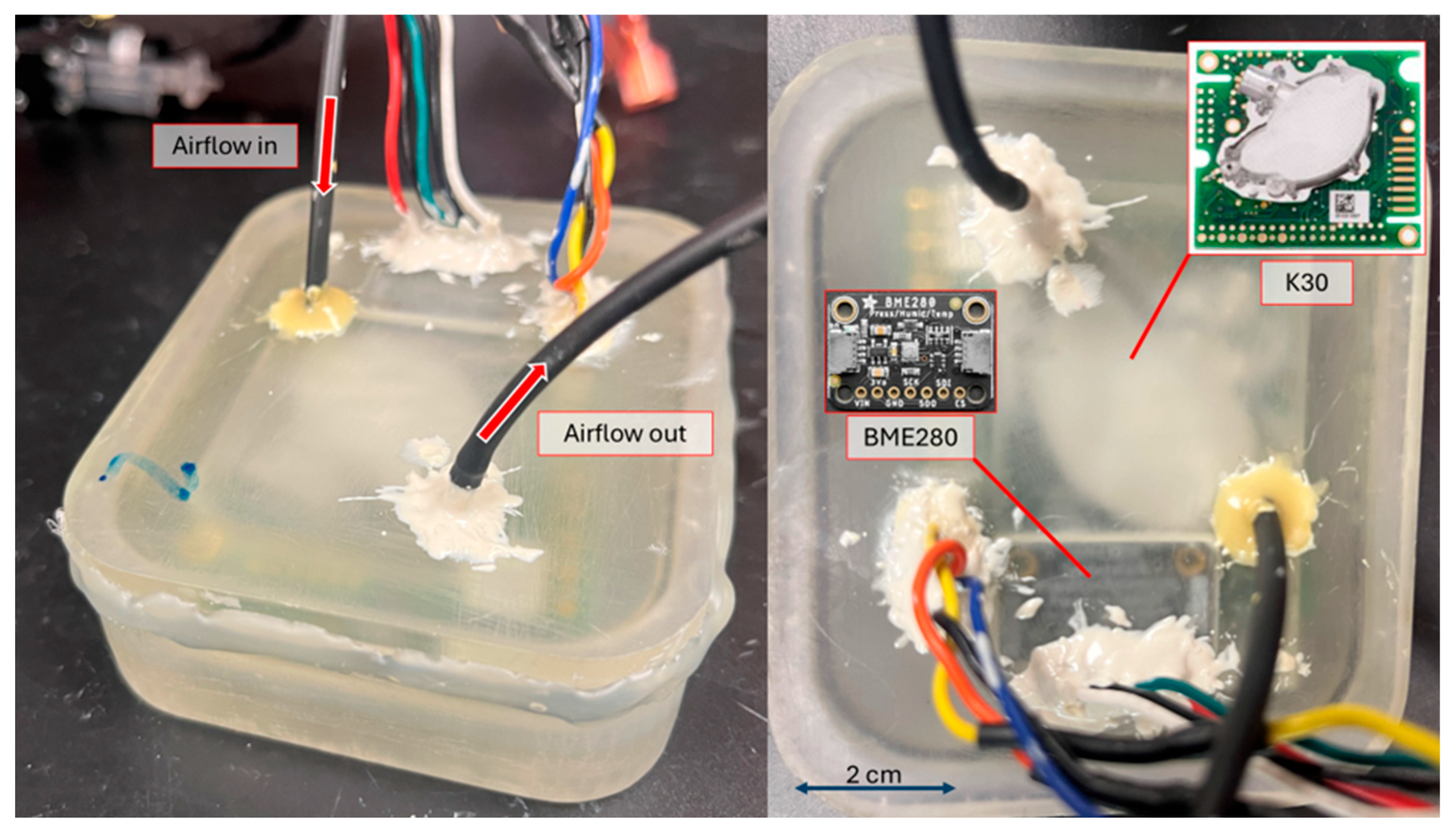
2.1.1. Internal Components

The SEACOW is designed to sit at the surface of the water, half submerged, and with one CO₂ exchanger in the air and one in the water. CO₂ permeates through expanded PTFE (ePTFE) membranes, enters an internal, sealed air stream, and flows through a solenoid valve, 61 cm of Nafion tubing placed inside ~160 g of Drierite desiccant, a gas pump, a 35 µm filter, into a custom K30 housing, and finally to a second 3-way solenoid valve (Figure 1). The solenoid valves are programmed to switch the air flow between the air-side exchanger and the water-side exchanger, depending on which side is being sampled at that time. Tubing was used for the water side of the SEACOW to decrease bubbles that could get trapped on the surface of the planar ePTFE when deployed.

2.1.2. Electronics and Software

The SEACOW hardware is composed of 11 electrical components, which are detailed in a circuit diagram with part numbers in Appendix A. However, the primary electrical components include the Boron microcontroller (Particle, San Francisco, CA, USA), the Adalogger Featherwing RTC+SD board (Adafruit, NYC, New York, NY, USA), and the K30 sensor (Senseair, Delsbo, Sweden). The Boron is the “brain” of the SEACOW, as it carries out the source code to control all other electrical components and powers the rest of the devices. The Boron is powered via a 3.7 V LiPo battery and can be communicated with via a micro-USB cable to update firmware. The source code for the Boron was developed using the Particle Workbench extension in Visual Studio Code version 1.95.3 and Particle Device OS 2.3.0.

The K30 is a non-dispersive infrared (NDIR) CO₂ sensor (USD 99) with an accuracy of ± 30 µatm or ± 3% of the reading (whichever is greater), which can be improved significantly with calibration [16,17,25,26]. While the K30 manual states it measures XCO₂, it was empirically determined by Wall (2014) that the K30 measures pCO₂, with which our group concurred after preliminary testing (in other words, the readings are proportional to pressure) [17]. Additionally, the K30 has an automatic baseline correction (ABC) algorithm that helps to deter long-term drift by assuming the lowest concentration measured in the last 7.5 days is the atmospheric level and corrects itself by shifting its readings. Therefore, we turned off the ABC algorithm prior to deployments using methods described in the K30 Modbus manual, since we were not measuring atmospheric values only, and therefore, lower values are possible [27]. We encased the K30, which has multiple gas inlets and outlets into the optical sensing path, in a custom 3D-printed housing and sealed it with marine epoxy to ensure airtightness and to control flow into and out of the sensor (Figure 2). Additionally, we placed a BME280 Protoboard (Adafruit, NYC, USA) inside the K30 housing to measure temperature, pressure, and humidity. This protoboard uses the BME280 sensor manufactured by Bosch Sensortec of Germany. The BME280 reads humidity with ± 3% accuracy, barometric pressure with ± 1 hPa absolute accuracy, and temperature with ± 1.0 °C accuracy. All materials used to build the SEACOW are listed on our GitHub repository (V1.0.1; https://doi.org/10.5281/zenodo.15122776).

The K30 communicates with a Boron microcontroller (Particle, San Francisco, CA, USA) over universal asynchronous receiver transmitter (UART) serial communication, which logs the readings to a micro-SD card on an Adalogger FeatherWing RTC + SD board (Adafruit, NYC, USA). All logged data can be downloaded from the micro-SD card by removing it from the Adalogger after deployment.

2.1.3. Outer Housing

The entire interior system, including all its electrical components, was secured onto an electronics tray with zip ties that slides into a 4-inch diameter schedule-80 PVC tube, which was polished to be O-ring smooth (600 grit emery cloth) to ensure a waterproof seal with the O-ring flanges. On both ends of the PVC tube, there was a watertight end cap secured into place with an O-ring flange (Blue Robotics, Torrance, CA, USA). We included a serpentine channel on the 3D-printed end cap on the air side to increase the surface area of the exchanger. The end cap was designed to be compatible with the existing O-ring flange from Blue Robotics after being polished. The ePTFE membrane (IPE, Tempe, AZ, USA) was placed on top of the serpentine channel and secured in place using a 3D-printed retainer and 4–40 machine screws (Figure 1). To measure air temperature, a TMP117 protoboard (Adafruit, NYC, USA), which uses the TMP117 sensor from Texas Instruments (Dallas, TX, USA), was placed inside a custom 3D-printed housing that fits onto a Blue Robotics cable penetrator. The TMP117 is sealed into its housing using marine epoxy except for a small portion where the actual sensing component of the TMP117 is exposed, which was covered in thermally conductive epoxy in order to keep all elements waterproof.

For the water-side cap, we 3D printed a tubing holder that fits on top of the aluminum end cap from Blue Robotics. The 1.85 mm inner diameter ePTFE tubing (IPE, AZ, USA) was coiled around the 3D-printed tubing holder and connected to two cable penetrators potted with barbed tubing and sealed with marine epoxy, which connects to the rest of the airstream (Figure 1). We placed a temperature sensor (I2C Fast Response, Blue Robotics) on this side to measure water temperature. All 3D designs, including the K30 housing, were printed in Formlabs clear resin using a Formlabs Form 3 printer (Boston, MA, USA) and are available on the SEACOW Github repository.

2.2. Characterizing the SEACOW

2.2.1. Air-Side Accuracy

Three additional SEACOWs were fabricated, and air-side measurements were compared between all four SEACOWs and those of a LI-850 (LI-COR Environmental, Lincoln, NE, USA). To assess their readings at a range of CO₂ concentrations (0–1500 ppm), the rates of industrial-grade N₂ and CO₂ gas (Airgas, PA, USA) flowing into a sealed mixing chamber (~12 L) were varied, using calculations detailed in Appendix B and mass flow controllers. We increased the CO₂ concentration by increments of ~250 ppm every 25 min. The air-tight mixing chamber was connected to the inputs and outputs of the LI-850 and the SEACOWs. Using the equilibrated readings from each SEACOW and the LI-850 at each step of the experiment, we produced dry calibrations (slope and intercept from a linear regression) for each SEACOW to fit the LI-850 data, which were then used in Equations (2)–(4), described below. The last 5 min of each step were deemed the equilibrated values. The LI-850 was calibrated prior to use according to instructions listed on LI-COR’s website [28].

2.2.2. Response Time

The LI-850 has a 90% response time of <3.5 s, which, for our purposes and relative to the slower K30 and SEACOW, we considered to be effectively instantaneous. Therefore, it was used to indicate when the mixing chamber reached the goal concentration and to compare its readings to the SEACOWs’ response time. To estimate the air-side response time of the SEACOW, the mixing chamber was flooded with 1500 ppm CO₂ until both the SEACOW and LI-850 stabilized. At a recorded time, the top of the box was removed and flooded with ambient air, facilitated with a fan. The time it took for each instrument to stabilize to the influx of ambient air was recorded, which provides an approximation of 5τ, or 99.3% response time, for the air side. Throughout the development process, we also repeated this process with several different potential diffusion membranes to evaluate their response times.

To estimate the 5τ time for the water side, a gas mixture of 1000 ppm CO₂ was bubbled into 2 L of deionized water for 24 h to produce water with elevated pCO₂. A stir plate and stir bar were used to ensure even mixing. Additionally, the gas mixture was bubbled first through a flask of deionized water prior to reaching the 2 L to humidify the gas stream and reduce evaporation. We placed the SEACOW, which had been sitting in air to equilibrate to the ambient room CO₂ concentrations, into the 2 L of high pCO₂ water and recorded the amount of time it took for the SEACOW to completely re-equilibrate as an estimate of the water-side 5τ time.

2.2.3. Humidity and Pressure Correction

We used the humidity, pressure, and temperature measurements from the BME280 sensor inside the K30 housing, as well as the water/air-side temperatures, to correct our K30 readings following methods by Wall (2014), which we updated for our lower humidity air stream [17]:

$$K{30}_{CO2}=[(K{30}_{raw}-K{30}_{H2O})\ast m_{dry}]+b$$

(2)

$$K{30}_{H2O}={(m}_{H2O}\ast V_{H2O}+b_{H2O})\ast (H/100)$$

(3)

$$V_{H2O}=6\ast {10}^{-5}(T^3)+5\ast {10}^{-4}(T^2)+0.055(T)+0.571$$

(4)

In these equations, $K{30}_{CO2}$ is the corrected CO₂ reading (µatm), $K{30}_{raw}$ is the reading before correction (µatm), $K{30}_{H2O}$ is the amount of the reading due to the presence of water vapor (µatm), $m_{dry}$ and b (µatm) are the slope and intercept of the dry calibration curve (as described in Section 2.2.1), $m_{H2O}$ (kPa µatm⁻¹) and $b_{H2O}$ (µatm) are the slope and intercept of the K30 reading vs. vapor pressure curve linear regression, H (%) is the relative humidity inside the K30 housing, $V_{H2O}$ is the vapor pressure of water (kPa), and $T$ (°C) is the water temperature. An example calculation using these equations can be found in the Supplemental Materials.

To obtain the $m_{H2O}$ and $b_{H2O}$ first, a flask of deionized water was placed inside a water bath (6200 R20, Fisher Scientific, Waltham, MA, USA) through which we bubbled industrial-grade N₂ gas to achieve a 100% humidity airstream, which fed into the K30 housing. The temperature of the water was varied from 18 to 24 °C to simulate a reasonable temperature range for the coast of North Carolina, and then the vapor pressure was calculated according to Equation (4). Once the vapor pressure values were calculated, a linear fit between vapor pressure and the K30 readings resulted in an $m_{H2O}$ and $b_{H2O}$ of −3.2 and 45 µatm, respectively. Note that no CO₂ gas was used in this step, so the entire response is due to H₂O.

This vapor pressure was calculated at a 100% humidity stream, but the inside the K30 housing only gets to 40–50% humidity during deployments due to the Nafion tubing and Drierite. Therefore, we multiply $K{30}_{H2O}$ by the proportion of the logged humidity to account for the fact that 100% humidity is not reached during actual deployments. We include the Drierite and Nafion tubing to ensure no moisture condenses on the internal electronics.

2.3. Laboratory Seagrass Experiment

A laboratory tank study was conducted in October 2023 to evaluate SEACOW’s ability to capture diel pCO₂ cycling. Two tanks (one “experimental” and one “control”) were used as follows. For the experimental tank, approximately 0.65 m² of Halodule wrightii was collected from a seagrass bed at 34.398° N, 77.616° W in September 2023 under UNCW CMS Collection DMF Permit #2037980 by coring the area to preserve the root system of the seagrass. Immediately following the coring, the seagrass and its sediment were placed into 4 rectangular plastic containers and placed into coolers, which were filled with seawater to avoid desiccation. Additionally, ≈45 L of sediment was collected from a seagrass-free area. The seagrass was placed in the experimental tank within 4 h of collection after its plastic container was further filled with the collected sediment to make sure it was securely planted. Sand (collected at 34.1934° N, 77.8047° W) was also sprinkled on top of the muddy sediment to decrease resuspension. The 95 L tank was filled with filtered seawater (<10 µm) to decrease the amount of biologically active material (i.e., living heterotrophs or autotrophs, which could influence CO₂ and O₂) in the tank. For the control tank, four more empty plastic containers were filled with the collected sediment and sand and placed in a different 95 L tank, which was also filled with the same filtered seawater. The experimental set up is pictured in Figure S4.

Each tank was outfitted with a hanging power filter (Qmax 90GPH), without the filter, to gently mix the water and a glass tank heater set to 22 °C, which is within the thermal optimal for H. wrightii [29]. Because the tanks received no additional water, they were prone to evaporation; accordingly, approximately 4 L of deionized water was added every 2–3 days to ensure the salinity of the tanks stayed consistently at 34–36 PSU. H. wrightii tolerates a wide range of salinities, from 25 to 45 PSU, with no changes in the growth rate; therefore, it was kept at an optimal range [29]. The tanks were uncovered. Four Finnex Planted+ (U-20WM; 23 W) aquarium lights were put on top of each tank to ensure sufficient lighting and were turned on from 6 am to 6 pm every day. One SEACOW and one dissolved oxygen (DO) sensor (miniDOT, PME, Vista, CA, USA) were placed in each tank. The SEACOW measured atmospheric pCO₂ for 8 min and then switched to sampling aquatic pCO₂ for 60 min at rate of 0.5 Hz. After sampling, it entered sleep mode for 52 min; consequently, one atmospheric and one aquatic pCO₂ value is measured every two hours. The dissolved oxygen sensor sampled every 2 min continuously. We then averaged the last 5 and 3 min of raw data for each water-side and air-side cycle, respectively, which are the equilibrated end points reported in the results.

3. Results

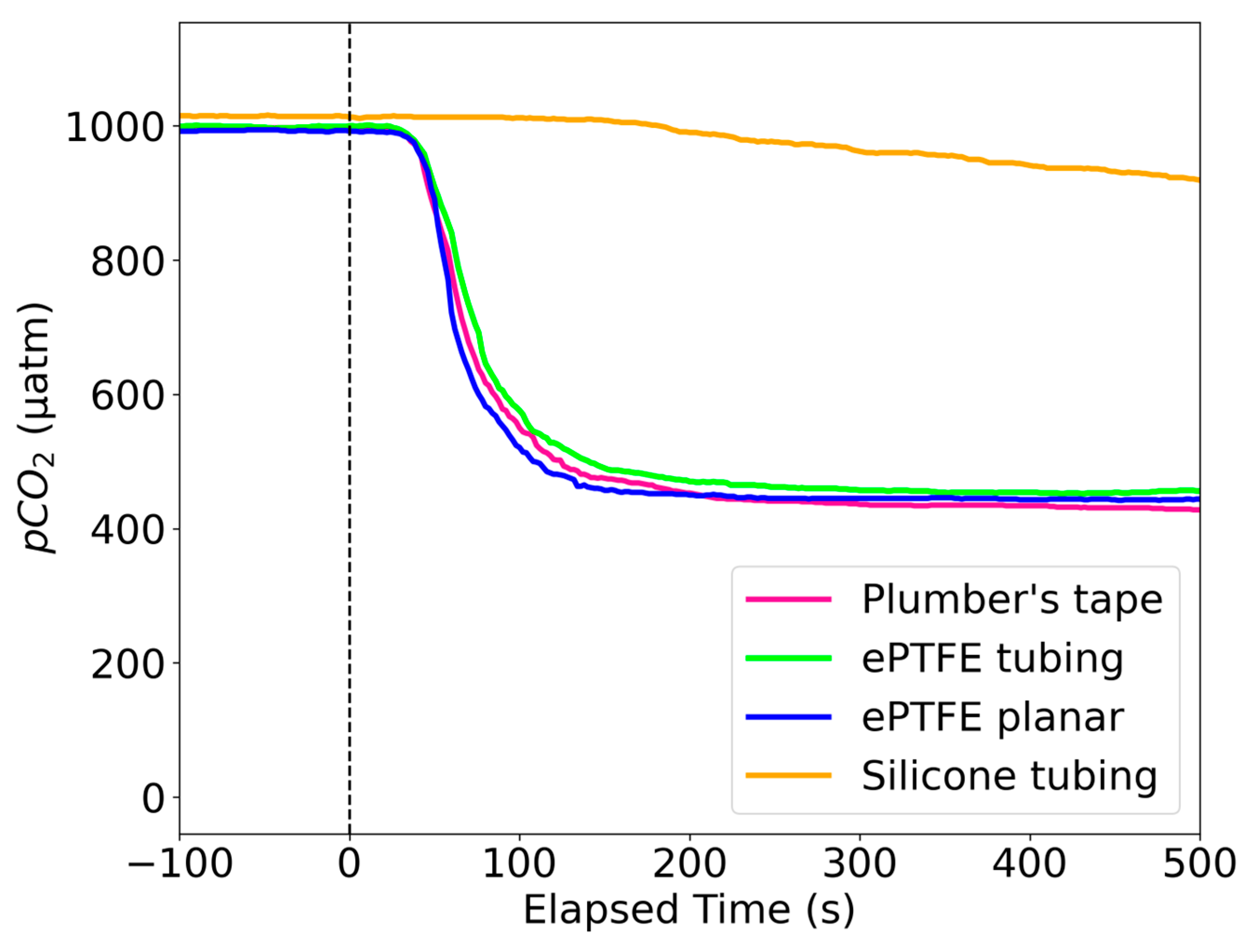
3.1. Response Times of Different Membranes

During the development process, the response times of several different potential diffusion membranes were evaluated by flooding a chamber with a known concentration of CO₂ and observing their response (Figure 3). The ePTFE (tubing 250 µm thick; planar 900 µm thick) had one of the fastest response times and higher durability than regular PTFE plumber’s tape (approx. 80 µm thick), so we chose it for our diffusion membranes. The silicone tubing we tested had a wall thickness of about 280 µm.

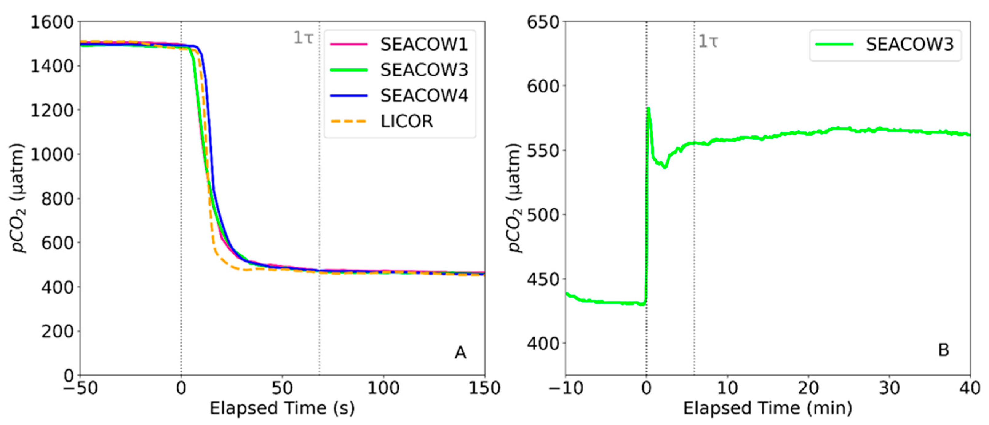
3.2. Air- and Water-Side Response Times

The averaged 99.3% air-side response time, or 5τ, of the SEACOW is 5.7 min, which we estimated by recording the amount of time it took for the SEACOWs to nearly equilibrate to the ambient air (Figure 4A). Therefore, 1τ is 1.14 min. It appears that there is not just a diffusion-limited response time but also a lag, likely due to “dead volume” in the system that needs to be flushed. It is important to note that the LI-850 did not have any diffusive barrier in place during this experiment and pumped at a rate of 0.75 L per minute. On the other hand, the SEACOW had the ePTFE planar diffusive membrane and pumps at a rate of about 0.20 L per minute. Note that SEACOW2 became inoperable due to a broken solenoid valve and was, therefore, excluded from the results. A more physically robust design to accommodate these or other solenoid valves could be introduced in the future design; however, it should be noted that we chose this particular solenoid valve because of its small size and low-power design.

The water-side response time (5τ) was calculated to be 29.6 min (Figure 4B). Only SEACOW3 was used during the water-side response time test due to spatial constraints in our tank. The equilibration of the water side is less stable than that of the air side, with a large spike occurring immediately after being placed in the water, which could be the result of the SEACOW being in close proximity to the operator’s breathing as it was placed. The general instability in the water-side response curve is likely caused by imperfections with our testing tank: the 2L container of DI water was open to the atmosphere while being bubbled with our gas mixture on a stir plate, potentially leading to small changes in aquatic pCO₂ happening faster than the SEACOW could measure. Additionally, the diffusion of CO₂ through water is slower than air, further contributing to the lag between the real time conditions and what the SEACOW was measuring. Additionally, the air stone used to bubble the 1000 µatm gas at a rate of 0.156 L min⁻¹ into the water may not have been sufficient for reaching the goal concentration. While the goal was for the water to reach 1000 µatm in order to compare to the SEACOW’s reading for accuracy as well as response time, we cannot say for certain what the CO₂ concentration of the water was without an independent measure and, therefore, used the data presented in Figure 4B to estimate the response time. Independent validation of water-side measurements would ideally occur through the comparison of aquatic SEACOW pCO₂ measurements to aquatic pCO₂ measured and/or estimated following best practices [30] and CO₂ system calculations (e.g., [31]). However, unfortunately, we did not have access to high-quality bench-top inorganic carbon analyzers. Nonetheless, the SEACOW’s NDIR gas sensor, the K30, measures CO₂ in the gas phase (Figure 2), and we thoroughly characterize gas-phase CO₂ measurements through comparisons between the K30 and LI-850 (see Section 3.3 Air-side accuracy), thereby providing a whole-system accuracy benchmark.

3.3. Air-Side Accuracy

A stepwise gas experiment was conducted to assess variations in K30 (and therefore SEACOW) performance “out of the box” and after calibration. Both pre- and post-calibration, the SEACOWs had standard deviations < 3 µatm (the majority of which were <1 µatm), demonstrating the instruments’ stability across the full range sampled (Figure 5).

After the dry calibration constants were applied (Appendix C), SEACOWs reported stabilized measurements to within ~2.5% (as percent difference) of the LI-850’s readings on average, excluding values at 0 µatm (Figure 5). After calibration, the root mean square errors for SEACOWs 1, 3, and 4 in comparison with LI-850’s values are 9.97, 21.66, and 19.80 µatm, respectively. Water-side accuracy has not been separately characterized thus far, but given the use of the same K30 sensing unit for both water- and air-side measurements and the same diffusion membrane type, no significant difference is expected. Moreover, given that the final measurement is a ∆pCO₂, any offset in the pCO₂ calculated from the K30 response should be cancelled out. We acknowledge, however, that a difference in sensor gain (e.g., the slope from the dry calibration curves) could contribute to inaccuracy as the ∆pCO₂ increases.

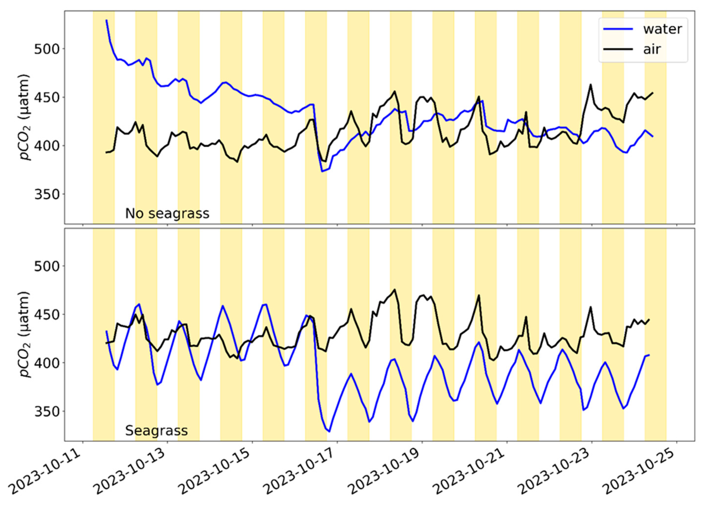
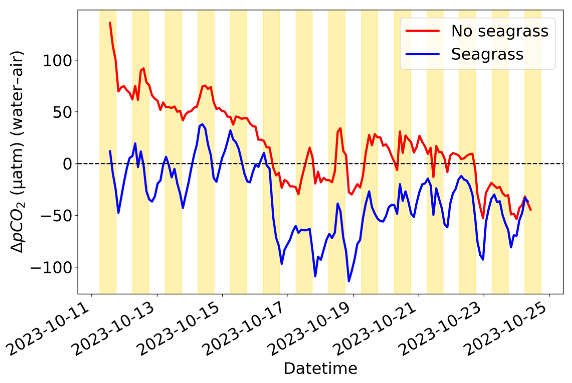
3.4. Seagrass Tank Experiment

SEACOWs collected ∆pCO₂ data successfully in two tanks for two weeks. SEACOW1 was in the control tank, while SEACOW3 and SEACOW4 were in the seagrass tank. Values from SEACOW3 are excluded from Figure 6 due to reporting unreliable data, caused by an internal air leak visible as a crack in a 3D-printed tubing connector. The more robust design implemented 1/16” plastic barbed tube connectors (e.g., Part 5047K71 from McMaster-Carr, Douglasville, GA, USA). Dissolved oxygen data were especially noisy in the no-seagrass tank and are shown in the Supplemental Materials. We suspect that small air bubbles may have been trapped on the surface of the DO sensor’s face. Both tanks (i.e., with and without seagrass) showed evidence of diel pCO₂ variability, likely due to the presence of a microbial community in the sediment. However, pCO₂ cycling is much more regular and amplified in the tank with seagrass (Figure 6), indicative of photosynthesis–respiration cycles. The lack of cycling in the DO readings in the no-seagrass tank also suggest that there was no consistent photosynthesis happening, presumably due to the lack of seagrass (Figure S1).

Throughout the experiment, the atmospheric pCO₂ decreased during the day and rose at night (Figure 6). Aquatic pCO₂ behaved as expected in the seagrass tank, with pCO₂ decreasing during the day as photosynthesis occurred and increasing during the night as respiration happened. There is a large decrease in aquatic pCO₂ on 16 October, which was due to the addition of deionized water to the tanks to maintain their salinity.

The difference between the averaged equilibrated water-side values and the air-side values was taken to produce ∆pCO₂ values (Figure 7). From 11 October to 16 October, the ∆pCO₂ values were as expected, with the seagrass tank seeing more consistent diel cycling, with values decreasing throughout the day and increasing through the night. Additionally, because the atmospheric pCO₂ values from both SEACOWs matched closely (Figure 6), most of the differences between the ∆pCO₂ values of each tank can be attributed to the aquatic pCO₂.

One of the main results of this project is the creation of the SEACOW itself, for which its characterization data are summarized below:

Note that the accuracy in

Table 1. Summary of characterization data for the SEACOW.

Characterization Parameter	Value
Accuracy	±2.5% of LI-850’s readings
Air-side 5τ time	5.7 min
Water-side 5τ time	~30 min
Power draw	185 mW
Drierite budget	162 g per 5 days
Temperature range	5–40 °C
Cost in parts	~1400 USD
Github design files [32]

was characterized in the range of 0 to 1500 µatm; therefore, the values reported here are only validated for CO₂ concentrations below 1500 µatm. However, the K30 sensor used in the SEACOW has a sampling range of 0–5000 µatm.

4. Discussion

Sampling pCO₂ in marine environments can be logistically difficult and expensive, yet it is a critical parameter to monitor as anthropogenic CO₂ continues to change the ocean chemistry. Not only does monitoring pCO₂ give scientists a better understanding of the quantity and effects of anthropogenic CO₂ uptake, but it allows scientists to study many different aspects of oceanography, such as the movement of water along the oceanic conveyor belt [12], the effect pCO₂ concentrations have on calcifying organisms [33], or the productivity of a region [34]. Additionally, there has been an increase in marine carbon dioxide removal (mCDR) groups who are looking for the best ways to monitor the movement of CO₂, so they can verify their methods of sequestering CO₂ from the atmosphere. Due to labor intensive and expensive methods of high-quality pCO₂ sensing, many of these groups and scientists are interested in low-cost pCO₂ technologies that can be deployed in larger quantities alongside more expensive, but singular, pCO₂ systems. In addition to developing pCO₂ monitoring for artificial carbon dioxide removal, it is important to monitor and protect blue carbon habitats that naturally sequester carbon, like seagrass meadows. Although we primarily discuss CO₂ sensing of coastal and oceanic environments in this paper, expensive aquatic pCO₂ sensors remain an issue for freshwater researchers as well, which has led to the development or application of similar instruments [24,35,36]. Furthermore, we acknowledge that the cost of the field instrument is comparably inexpensive, but some of the lab equipment needed for characterization (e.g., LI-850, gas tanks, 3D printer, and water bath) of this build increases the cost.

During deployments, we identified several areas of improvement for the SEACOW. Although the response time for the air side is sufficient for capturing rapid changes in atmospheric CO₂ during deployments, the water-side response time is not as competitive when compared to other pCO₂ instruments. The SIPCO₂ (accuracy 29  ±  6 μatm) [16] and the CO2-Pro (accuracy ± 0.5%) (Pro-Oceanus) have reported approximate 5τ response times of 15 min and 12.5 min, respectively. The CO2-Pro’s efficient response time could be attributed to its pump that moves water across the equilibration membrane, which also reduces biofouling but increases its power consumption. The SEACOW’s water-side response time could be accelerated by adding an external pump or stirring mechanism, which may also assist in preventing biofouling. Additional research could also focus on improving the exchanger material and/or geometry (i.e., a higher surface area to volume ratio) as well as the rate of pumped air to assist with CO₂ permeation [37]. We also note that Formlabs does not supply resin chemistry, and we, therefore, do not know what its CO₂ permeability/absorptivity properties are for our 3D parts. However, given these results and the overall accuracy of the instrument, we do not consider this to be a significant source of uncertainty or response time lag. Additionally, we acknowledge that the lack of independent measurements of aquatic pCO₂ during the water-side response time experiment results in uncertainty of the robustness of water-side measurements. In future developments of the SEACOW, resolving the water-side accuracy will be paramount. Additionally, we focus on data from one laboratory deployment in this paper (e.g., the seagrass experiment); therefore, it is imperative that future work focuses on replicating these types of experiments and performing other field deployments to assess the reliability of the system.

Finally, for the SEACOW to be used as an autonomous field instrument, the most pressing improvements for future deployments are the addition of a solar panel or larger battery pack, adding more Drierite to the system/using a different drying mechanism, and decreasing biofouling. When deployed in the field, the ePTFE tubing on the water side of the SEACOW became covered in algae after ~7 days; however, we found that rinsing the ePTFE tubing with deionized water from a wash bottle with a pointed nozzle was effective in removing the algae without damaging the ePTFE tubing. Currently, the Drierite is the biggest limitation for length of field deployments, becoming saturated after approximately 5 days of use. Depending on the application, the SEACOW could be modified to include a drying gas to extend this period. These advancements would allow the SEACOW to be deployed alongside more robust systems to increase spatial resolution of sampling. A possible design of a simple, low-cost float to deploy the SEACOW at the air–water interface is pictured in Figure S5. Additionally, the SEACOW may be secured to a floating dock for deployments.

5. Conclusions

In this project, we designed and built a ∆pCO₂ device, characterized its functionality, and demonstrated its ability to capture the diel pCO₂ cycling of seagrass in a controlled environment. The increasing popularity of microcontrollers and off-the-shelf parts help improve accessibility of monitoring technologies, which was one of the major goals of this project. We acknowledge that there are several improvements to be made on the SEACOW, and in the future, work will be focused on improving overall system accuracy characterization, decreasing the water-side response time, repeating characterization experiments and field deployments, and making the instrument more robust for longer field deployments. The work presented here further aids in characterizing the K30, which is increasingly popular in other low-cost atmospheric and/or aquatic CO₂-sensing technologies. Because the SEACOW measures atmospheric and aquatic pCO₂, a ∆pCO₂ (pCO_2(water)-pCO_2(air)) value can be obtained and used to calculate CO₂ fluxes. Therefore, even if the K30 sensor readings start to drift over time, the drift is subtracted out when the difference is taken, allowing the SEACOW to maintain rigor during deployments. This feature, along with the fact that the parts cost USD ~1400, make the SEACOW a valuable contribution to biogeochemical scientific and engineering communities.

References

1. Friedlingstein, P.; O’Sullivan, M.; Jones, M.W.; Andrew, R.M.; Hauck, J.; Landschützer, P.; Le Quéré, C.; Li, H.; Luijkx, I.T.; Olsen, A. Global carbon budget 2024. Earth Syst. Sci. Data Discuss. 2024, 2024, 1–133. [Google Scholar] [CrossRef]
2. Dai, M.; Su, J.; Zhao, Y.; Hofmann, E.E.; Cao, Z.; Cai, W.-J.; Gan, J.; Lacroix, F.; Laruelle, G.G.; Meng, F.; et al. Carbon Fluxes in the Coastal Ocean: Synthesis, Boundary Processes, and Future Trends. Annu. Rev. Earth Planet. Sci. 2022, 50, 593–626. [Google Scholar] [CrossRef]
3. Bauer, J.E.; Cai, W.-J.; Raymond, P.A.; Bianchi, T.S.; Hopkinson, C.S.; Regnier, P.A.G. The changing carbon cycle of the coastal ocean. Nature 2013, 504, 61–70. [Google Scholar] [CrossRef]
4. Takahashi, T.; Olafsson, J.; Goddard, J.G.; Chipman, D.W.; Sutherland, S. Seasonal variation of CO2 and nutrients in the high-latitude surface oceans: A comparative study. Glob. Biogeochem. Cycles 1993, 7, 843–878. [Google Scholar] [CrossRef]
5. Lefèvre, N.; Watson, A.J.; Cooper, D.J.; Weiss, R.F.; Takahashi, T.; Sutherland, S.C. Assessing the seasonality of the oceanic sink for CO2 in the northern hemisphere. Glob. Biogeochem. Cycles 1999, 13, 273–286. [Google Scholar] [CrossRef]
6. Gregor, L.; Shutler, J.; Gruber, N. High-resolution variability of the ocean carbon sink. Glob. Biogeochem. Cycles 2024, 38, e2024GB008127. [Google Scholar] [CrossRef]
7. Herr, D.; Landis, E. Coastal Blue Carbon Ecosystems. Opportunities for Nationally Determined Contributions; Policy Brief; IUCN: Gland, Switzerland; TNC: Washington, DC, USA, 2016. [Google Scholar]
8. Fourqurean, J.W.; Duarte, C.M.; Kennedy, H.; Marbà, N.; Holmer, M.; Mateo, M.A.; Apostolaki, E.T.; Kendrick, G.A.; Krause-Jensen, D.; Mcglathery, K.J.; et al. Seagrass ecosystems as a globally significant carbon stock. Nat. Geosci. 2012, 5, 505–509. [Google Scholar] [CrossRef]
9. Macreadie, P.; Baird, M.; Trevathan-Tackett, S.; Larkum, A.; Ralph, P. Quantifying and modelling the carbon sequestration capacity of seagrass meadows—A critical assessment. Mar. Pollut. Bull. 2014, 83, 430–439. [Google Scholar] [CrossRef]
10. Resplandy, L.; Hogikyan, A.; Müller, J.; Najjar, R.; Bange, H.W.; Bianchi, D.; Weber, T.; Cai, W.J.; Doney, S.; Fennel, K. A synthesis of global coastal ocean greenhouse gas fluxes. Glob. Biogeochem. Cycles 2024, 38, e2023GB007803. [Google Scholar] [CrossRef]
11. Watson, A.J.; Schuster, U.; Shutler, J.D.; Holding, T.; Ashton, I.G.; Landschützer, P.; Woolf, D.K.; Goddijn-Murphy, L. Revised estimates of ocean-atmosphere CO2 flux are consistent with ocean carbon inventory. Nat. Commun. 2020, 11, 4422. [Google Scholar] [CrossRef]
12. Takahashi, T.; Sutherland, S.C.; Wanninkhof, R.; Sweeney, C.; Feely, R.A.; Chipman, D.W.; Hales, B.; Friederich, G.; Chavez, F.; Sabine, C. Climatological mean and decadal change in surface ocean pCO2, and net sea–air CO2 flux over the global oceans. Deep Sea Res. Part II Top. Stud. Oceanogr. 2009, 56, 554–577. [Google Scholar]
13. Rosentreter, J.A. Water-air gas exchange of CO2 and CH4 in coastal wetlands. In Carbon Mineralization in Coastal Wetlands; Elsevier: Amsterdam, The Netherlands, 2022; pp. 167–196. [Google Scholar]
14. Wanninkhof, R. Relationship between gas exchange and wind speed over the ocean. J. Geophys. Res. 1992, 97, 7373–7381. [Google Scholar] [CrossRef]
15. Wanninkhof, R.; Asher, W.E.; Ho, D.T.; Sweeney, C.; McGillis, W.R. Advances in quantifying air-sea gas exchange and environmental forcing. Annu. Rev. Mar. Sci. 2009, 1, 213–244. [Google Scholar] [CrossRef] [PubMed]
16. Hunt, C.W.; Snyder, L.; Salisbury, J.E.; Vandemark, D.; Mcdowell, W.H. SIPCO2: A simple, inexpensive surface water pCO2 sensor. Limnol. Oceanogr. Methods 2017, 15, 291–301. [Google Scholar] [CrossRef]
17. Wall, C.M. Autonomous In Situ Measurements of Estuarine Surface PCO2: Instrument Development and Initial Estuarine Observations. Master’s Thesis, Oregon State University, Corvallis, OR, USA, 2014. [Google Scholar]
18. Graziani, S.; Beaubien, S.E.; Bigi, S.; Lombardi, S. Spatial and temporal pCO2 marine monitoring near Panarea Island (Italy) using multiple low-cost GasPro sensors. Environ. Sci. Technol. 2014, 48, 12126–12133. [Google Scholar] [CrossRef]
19. Ge, X.; Kostov, Y.; Henderson, R.; Selock, N.; Rao, G. A low-cost fluorescent sensor for pCO2 measurements. Chemosensors 2014, 2, 108–120. [Google Scholar] [CrossRef]
20. Pan, C.; Patel, V.; Gewirtzman, J.; Richardson, I.; Dubey, R.; Caylor, K.; Dollar, A.; Forbes, E. Fluxbot: The Next Generation-Design and Validation of a Wireless, Open-Source Mechatronic CO2 Flux Sensing Chamber. In Proceedings of the 7th ACM SIGCAS/SIGCHI Conference on Computing and Sustainable Societies, New Delhi, India, 8–11 July 2024; pp. 85–96. [Google Scholar]
21. Sabine, C.; Sutton, A.; Mccabe, K.; Lawrence-Slavas, N.; Alin, S.; Feely, R.; Jenkins, R.; Maenner, S.; Meinig, C.; Thomas, J.; et al. Evaluation of a New Carbon Dioxide System for Autonomous Surface Vehicles. J. Atmos. Ocean. Technol. 2020, 37, 1305–1317. [Google Scholar] [CrossRef]
22. Nicholson, D.P.; Michel, A.P.M.; Wankel, S.D.; Manganini, K.; Sugrue, R.A.; Sandwith, Z.O.; Monk, S.A. Rapid Mapping of Dissolved Methane and Carbon Dioxide in Coastal Ecosystems Using the ChemYak Autonomous Surface Vehicle. Environ. Sci. Technol. 2018, 52, 13314–13324. [Google Scholar] [CrossRef]
23. Sutton, A.J.; Sabine, C.L.; Maenner-Jones, S.; Lawrence-Slavas, N.; Meinig, C.; Feely, R.A.; Mathis, J.T.; Musielewicz, S.; Bott, R.; Mclain, P.D.; et al. A high-frequency atmospheric and seawater pCO2 data set from 14 open-ocean sites using a moored autonomous system. Earth Syst. Sci. Data 2014, 6, 353–366. [Google Scholar] [CrossRef]
24. Johnson, M.S.; Billett, M.F.; Dinsmore, K.J.; Wallin, M.; Dyson, K.E.; Jassal, R.S. Direct and continuous measurement of dissolved carbon dioxide in freshwater aquatic systems-method and applications. Ecohydrology 2009, 3, 68–78. [Google Scholar] [CrossRef]
25. Yasuda, T.; Yonemura, S.; Tani, A. Comparison of the Characteristics of Small Commercial NDIR CO2 Sensor Models and Development of a Portable CO2 Measurement Device. Sensors 2012, 12, 3641–3655. [Google Scholar] [CrossRef] [PubMed]
26. Martin, C.R.; Zeng, N.; Karion, A.; Dickerson, R.R.; Ren, X.; Turpie, B.N.; Weber, K.J. Evaluation and environmental correction of ambient CO2 measurements from a low-cost NDIR sensor. Atmos. Meas. Tech. 2017, 10, 2383–2395. [Google Scholar] [CrossRef] [PubMed]
27. Senseair AB. Modbus on Senseair K30, Senseair K33 and eSENSE; Document TDE2336; Senseair AB: Delsbo, Sweden, 2023; 19p. [Google Scholar]
28. LI-COR. Maintenance on LI-850 and LI-830 Analyzers. Available online: https://www.licor.com/support/LI-850/topics/maintenance.html (accessed on 16 July 2024).
29. Mazzotti, F.J.; Pearlstine, L.G.; Chamberlain, R.; Barnes, T.; Chartier, K.; DeAngelis, D. Stressor Response Models for Seagrasses, Halodule Wrightii and Thalassia Testudnium; University of Florida, Florida Lauderdale Research and Education Center: Fort Lauderdale, FL, USA, 2007; p. 19. [Google Scholar]
30. Dickson, A.G.; Sabine, C.L.; Christian, J.R. Guide To Best Practices for Ocean CO2 Measurements; North Pacific Marine Science Organization: Sidney, BC, Canada, 2007. [Google Scholar]
31. Van Heuven, S.; Pierrot, D.; Rae, J.; Lewis, E.; Wallace, D. MATLAB Program Developed for CO2 System Calculations; Carbon Dioxide Information Analysis Center (CDIAC): Oak Ridge, TN, USA, 2011. [Google Scholar]
32. Farquhar, E.; Bresnahan, P.; Tydings, M.; Portelli, D. COAST-Lab/SEACOW_Public: V1.0.1. 2025. Available online: https://zenodo.org/records/15122776 (accessed on 2 April 2025).
33. Fujita, K.; Hikami, M.; Suzuki, A.; Kuroyanagi, A.; Sakai, K.; Kawahata, H.; Nojiri, Y. Effects of ocean acidification on calcification of symbiont-bearing reef foraminifers. Biogeosciences 2011, 8, 2089–2098. [Google Scholar] [CrossRef]
34. Körtzinger, A.; Send, U.; Lampitt, R.; Hartman, S.; Wallace, D.W.; Karstensen, J.; Villagarcia, M.; Llinás, O.; DeGrandpre, M. The seasonal pCO2 cycle at 49 N/16.5 W in the northeastern Atlantic Ocean and what it tells us about biological productivity. J. Geophys. Res. Ocean. 2008, 113, C04020. [Google Scholar] [CrossRef]
35. Bastviken, D.; Sundgren, I.; Natchimuthu, S.; Reyier, H.; Gålfalk, M. Cost-efficient approaches to measure carbon dioxide (CO2) fluxes and concentrations in terrestrial and aquatic environments using mini loggers. Biogeosciences 2015, 12, 3849–3859. [Google Scholar] [CrossRef]
36. Robison, A.L.; Koenig, L.E.; Potter, J.D.; Snyder, L.E.; Hunt, C.W.; McDowell, W.H.; Wollheim, W.M. Lotic-SIPCO2: Adaptation of an open-source CO2 sensor system and examination of associated emission uncertainties across a range of stream sizes and land uses. Limnol. Oceanogr. Methods 2024, 22, 191–207. [Google Scholar] [CrossRef]
37. Lee, D.J.J.; Kek, K.T.; Wong, W.W.; Mohd Nadzir, M.S.; Yan, J.; Zhan, L.; Poh, S.C. Design and optimization of wireless in-situ sensor coupled with gas–water equilibrators for continuous pCO2 measurement in aquatic environments. Limnol. Oceanogr. Methods 2022, 20, 500–513. [Google Scholar] [CrossRef]
Figure 1. The plumbing diagram using ePTFE as a planar exchanger for the air side and ePTFE tubing for the water side. The red arrows indicate the direction of air flow. The components in the gray shaded region are the interior components of the device, the assembled version of which is shown on the right-hand side. The use of ePTFE as the exchanger was inspired by methods used in previous studies [24]. Once fully assembled, the SEACOW itself, shown in the right side of the figure, is 29.2 cm long with a diameter of 10.16 cm.
Sensors 25 03547 g001
Figure 2. The 3D-printed K30 housing. The wire holes and top are sealed with marine epoxy to reduce gas leaks. It is 8.7 cm × 7.5 cm × 2.7 cm. The wires shown here are the communication and power to the BME280 and K30 sensors, which are housed inside. A scale is shown on the right-hand image.
Sensors 25 03547 g002
Figure 3. Response time of several semipermeable membranes to a change in pCO2 occurring at time 0.
Sensors 25 03547 g003
Figure 4. (A) The response of the SEACOWs air side to a step change in pCO2 occurring at time 0. Note that the x-axis has been limited to 150 s in order to emphasize the response within 1τ, as opposed to the full 5τ response. (B) The response of the SEACOW to a step change in aquatic pCO2 at time 0.
Sensors 25 03547 g004
Figure 5. (A) Stepwise gas experiment of all four SEACOWs vs. the LI-COR LI-850 prior to applying the dry calibration curves. LI-COR LI-850 XCO2 measurements were converted to pCO2 for comparison. The dotted gray line represents the CO2 concentration set points throughout the experiment. (B) Stepwise gas experiment after applying the dry calibration curves. (C) The averages of the last 5 min of each ‘”step” plotted against their line of best fit, or the dry calibration curve, which are labeled using matching color. Error bars indicating standard deviation within the final five minutes were excluded from (C,D) due to being smaller than the markers and, therefore, not visible, so the data presented in these two panels can be found in table form in Appendix C. (D) The averages of the last 5 min of each “step” after applying the dry calibration curve. The orange 1-to-1 line is plotted using the data from LICOR averages as the x and y values.
Sensors 25 03547 g005
Figure 6. Equilibrated pCO2 end points plotted for the air (black) and water sides (blue) for the tanks with and without seagrass, as labeled. Yellow background signifies “daytime,” or when the aquarium lights are illuminated, and white background signifies “nighttime,” or when lights are turned off.
Sensors 25 03547 g006
Figure 7. ∆pCO2 (water–air) values for SEACOW1 and 4, which were in the control tank and seagrass tank, respectively.
Sensors 25 03547 g007