

Deep Edge-Based Fault Detection for Solar Panels

Abstract
1. Introduction
- We develop a novel fault detection pipeline of solar panels, which consists of three steps: (a) edge detection, (b) contour filter, and (c) classification.
- We adapt existing CNNs for fault detection of solar panels. To the best of our knowledge, ours is the first CNN-based edge detection approach in this task. The proposed bottom–up self-attention structure leads to more detailed edge location information.
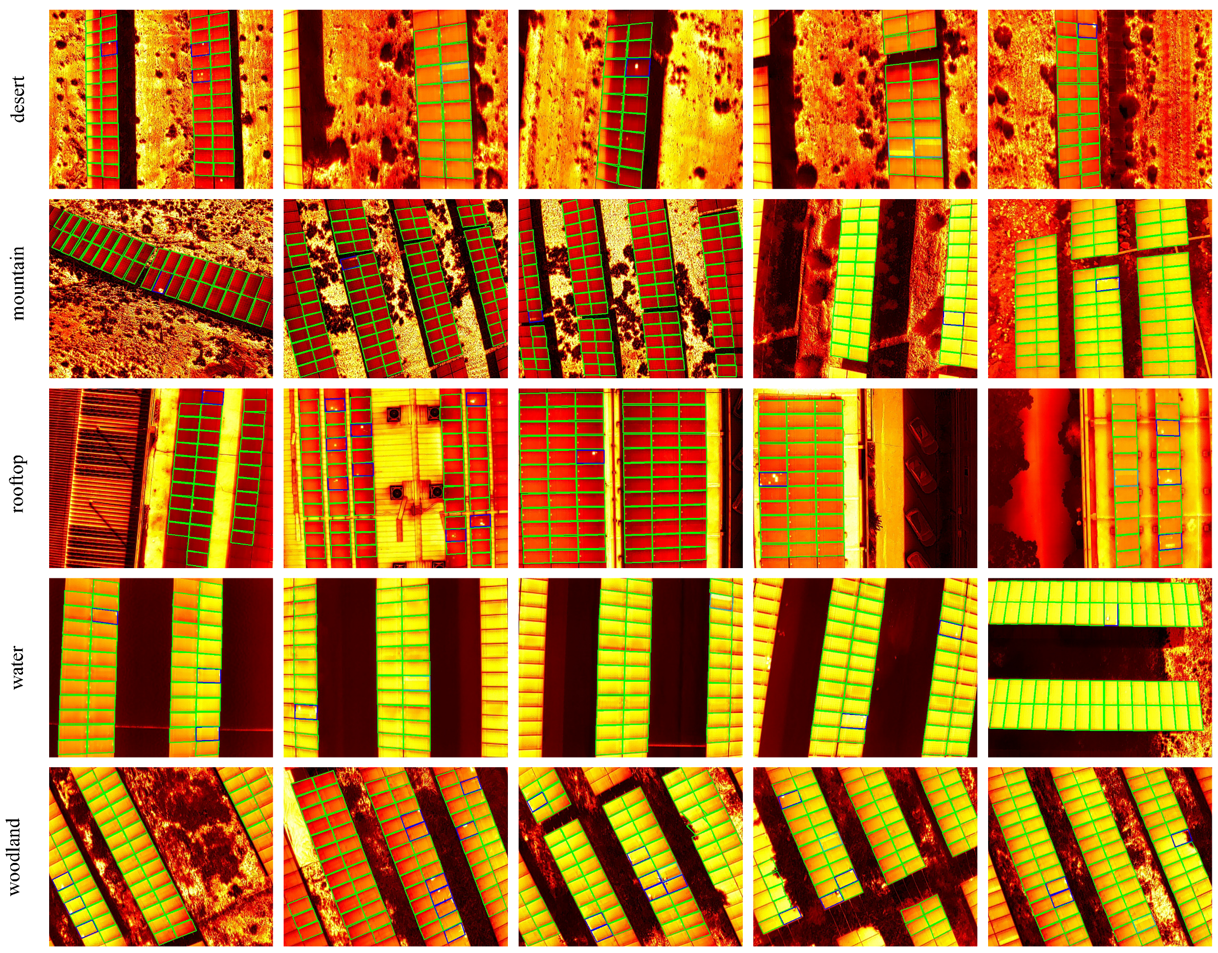
- We collect and annotate 1200 images in different photovoltaic power plants (desert, mountain, roof, water, woodland) and achieve a high macro F1 score in 860 testing images.
2. Related Work
2.1. Edge Detection
2.2. Fault Detection of PV Panels
3. Materials and Methods
3.1. Edge Detection
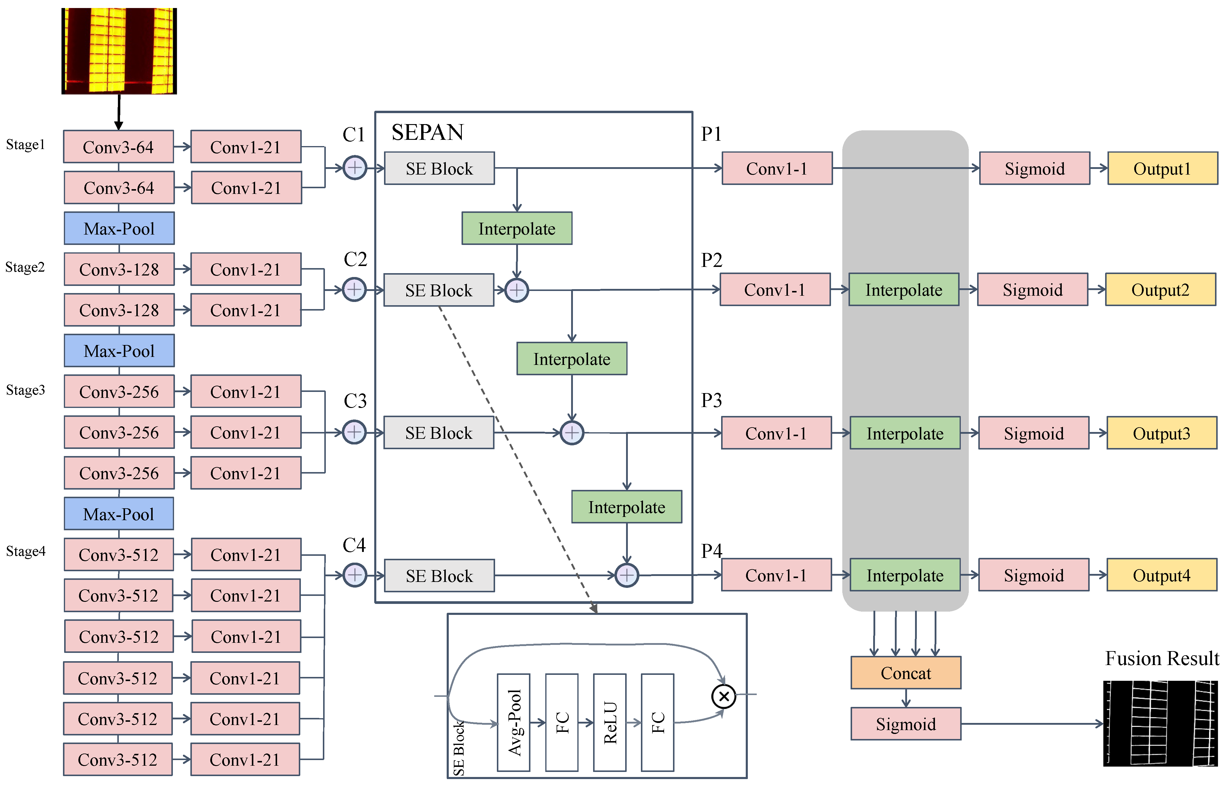
3.1.1. Backbone
3.1.2. Squeeze-and-Excitation Path Aggregation Structure
3.1.3. Loss Function
3.2. Contour Filter
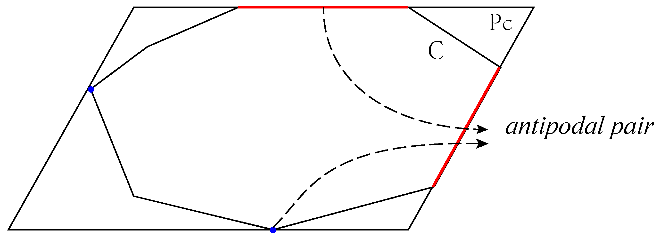
3.2.1. Minimal Enclosing Parallelogram
- Obtain the list by the Rotating Calipers algorithm, where vertex is the farthest from edge among all the vertices of C;
- Sequentially traverse the list L and select and to determine the unique parallelogram ;
- Repeat Step 2 until all candidate parallelograms have been processed.
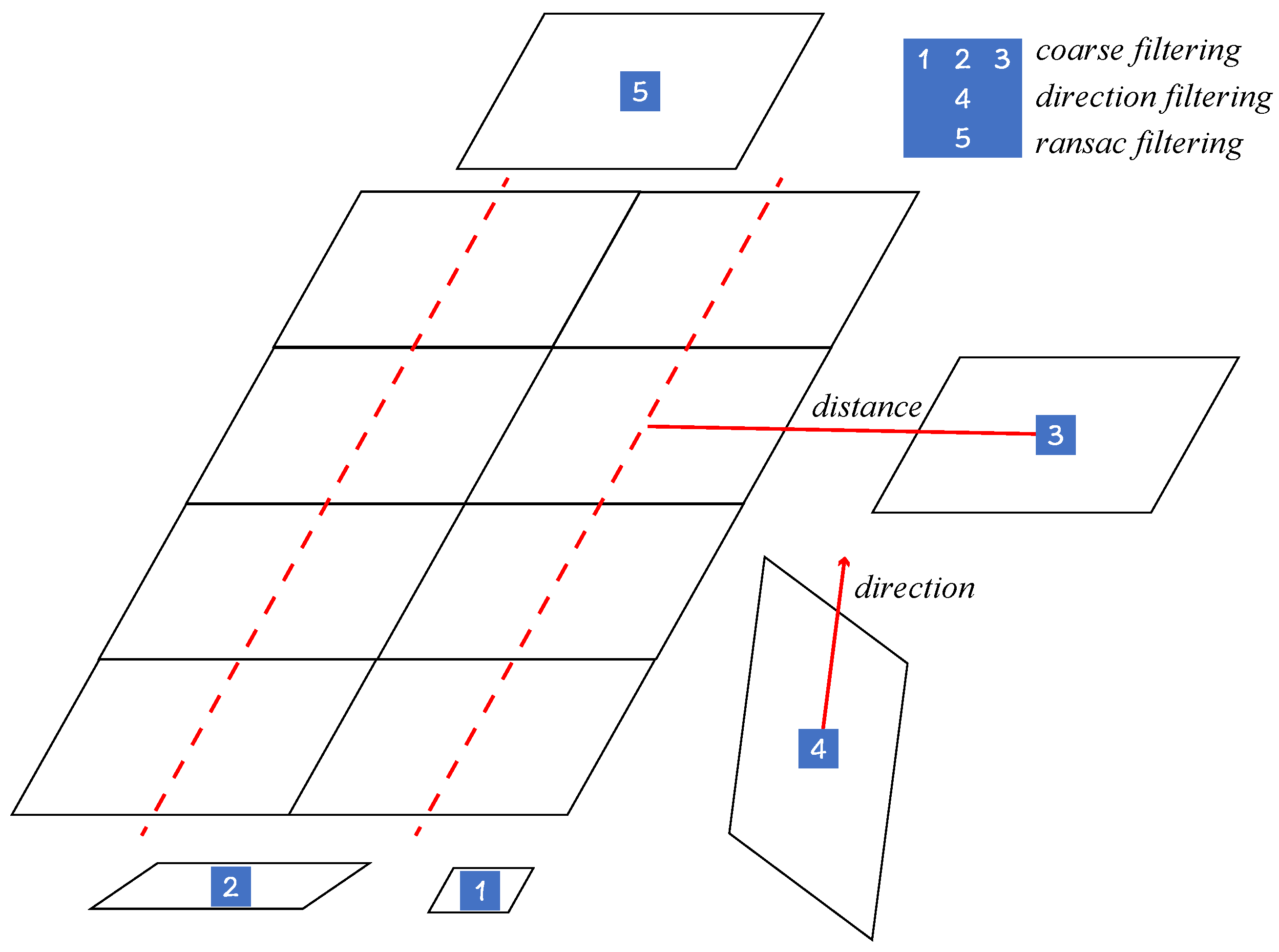
3.2.2. Coarse Filter
- Filter those parallelograms, e.g., No. 1 in Figure 3, that do not satisfy , where is the area of , and and are preset thresholds;
- Exclude parallelograms, e.g., No. 2 in Figure 3, when the aspect ratio is larger than a threshold , where and represent the short side and the long side of , respectively;
- Filter those parallelograms, e.g., No. 3 in Figure 3, without candidates nearby, i.e., those parallelograms whose distance to that parallelogram is greater than a threshold .
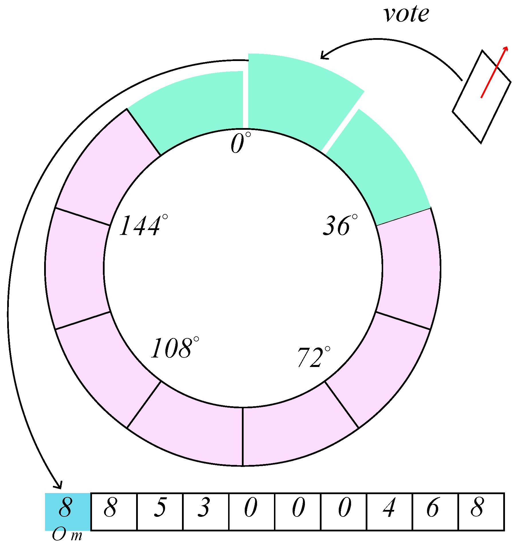
3.2.3. Main Direction Filter
- Divide the range of equally into grids ;
- Update the scores of the grid , which belongs to, and its neighboring grids , where is the threshold of the voting strategy;
- The direction of the highest scoring grid is taken as the main direction . Filter parallelograms that do not satisfy the condition .
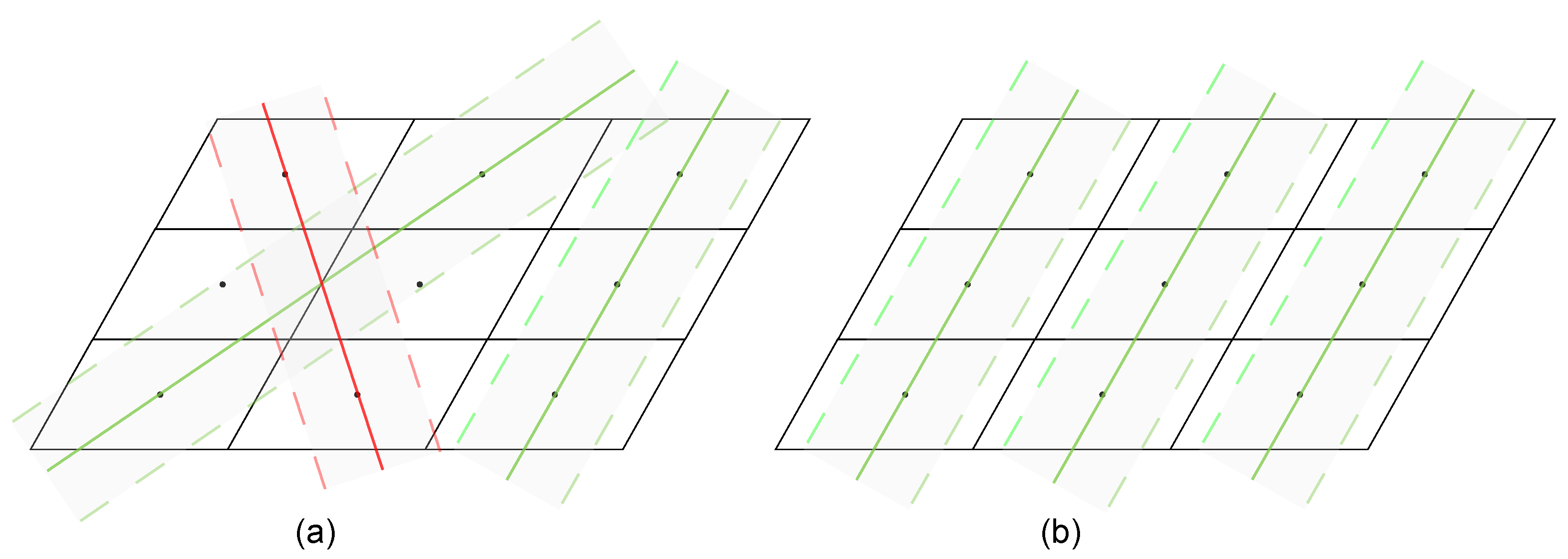
3.2.4. RANSAC Filter
- Find an optimal straight line l using the standard RANSAC algorithm, which has the maximum number of interior points;
- Remove the interior points of line l from set S to obtain set ;
- Repeat the above steps until . Then filter the optimal line with the number of interior points less than the threshold .
- For each centroid , choose two lines and , where and represent the direction of the long and short axes of the parallelogram , respectively;
- Calculate the number of interior points of lines, where and have interior point thresholds of and ;
- Select one of the optimal straight lines l. Since there is an overlap of the interior points of the lines, it is necessary to remove those interior points that are part of the optimal line among the interior points of the non-optimal lines;
- Repeat Step 3 until all centroids are assigned to an optimal line, filtering out the optimal lines whose number of interior points is less than the threshold .
3.3. Classification
- Normal solar panels, ;
- Rectangular hotspots, ;
- Dotted hotspots, otherwise.
4. Experimental Results
4.1. Datasets and Implementation
4.2. Results on Solar Panel Image Dataset
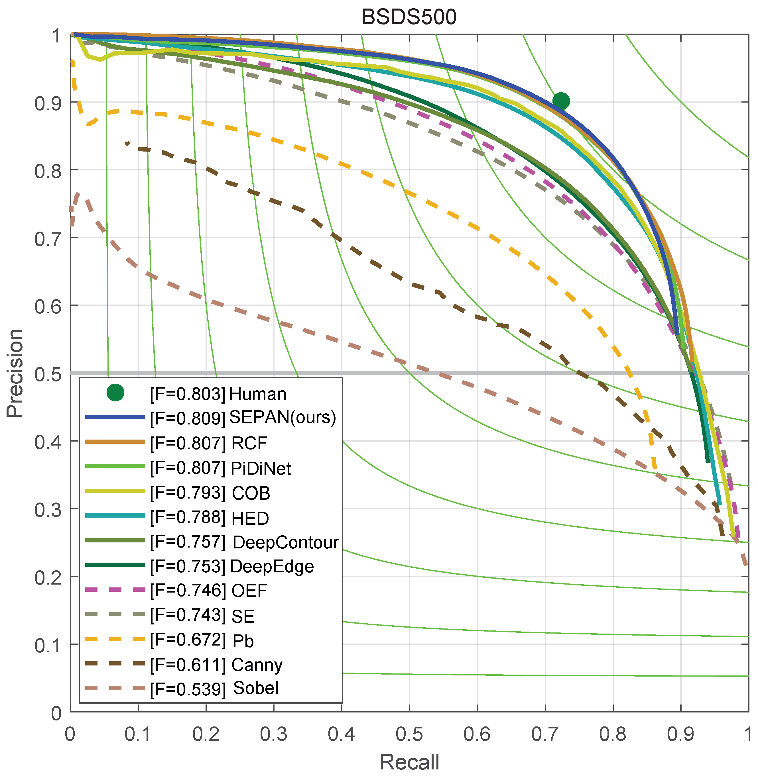
4.3. Results on BSDS500
5. Conclusions
Author Contributions
Funding
Institutional Review Board Statement
Informed Consent Statement
Data Availability Statement
Conflicts of Interest
References
- Ram, M.; Bogdanov, D.; Aghahosseini, A.; Gulagi, A.; Oyewo, A.S.; Child, M.; Caldera, U.; Sadovskaia, K.; Farfan, J.; Barbosa, L.S.N.S.; et al. Global Energy System Based on 100% Renewable Energy—Power, Heat, Transport and Desalination Sectors; Lappeenranta University of Technology: Lappeenranta, Finland; Energy Watch Group: Berlin, Germany, 2019. [Google Scholar]
- Venkatesh S, N.; Sugumaran, V. Fault diagnosis of visual faults in photovoltaic modules: A Review. Int. J. Green Energy 2020, 18, 37–50. [Google Scholar]
- Madeti, S.R.; Singh, S.N. A comprehensive study on different types of faults and detection techniques for solar photovoltaic system. Sol. Energy 2017, 158, 161–185. [Google Scholar] [CrossRef]
- Bhaskaranand, M.; Gibson, J.D. Low-complexity video encoding for UAV reconnaissance and surveillance. In Proceedings of the 2011-MILCOM 2011 Military Communications Conference, Baltimore, MD, USA, 7–10 November 2011. [Google Scholar]
- Barbedo, J.G.A.; Koenigkan, L.V.; Santos, T.T.; Santos, P.M. A study on the detection of cattle in UAV images using deep learning. Sensors 2019, 19, 5436. [Google Scholar] [CrossRef]
- Sa, I.; Hrabar, S.; Corke, P. Outdoor flight testing of a pole inspection UAV incorporating high-speed vision. In Field and Service Robotics; Springer: Cham, Switzerland, 2015. [Google Scholar]
- Su, B.; Chen, H.; Liu, K.; Liu, W. RCAG-Net: Residual Channelwise Attention Gate Network for Hot Spot Defect Detection of Photovoltaic Farms. IEEE Trans. Instrum. Meas. 2021, 70, 1–14. [Google Scholar] [CrossRef]
- Akram, M.W.; Li, G.; Jin, Y.; Chen, X.; Zhu, C.; Ahmad, A. Automatic detection of photovoltaic module defects in infrared images with isolated and develop-model transfer deep learning. Sol. Energy 2020, 198, 175–186. [Google Scholar] [CrossRef]
- Dotenco, S.; Dalsass, M.; Winkler, L.; Würzner, T.; Brabec, C.; Maier, A.; Gallwitz, F. Automatic detection and analysis of photovoltaic modules in aerial infrared imagery. In Proceedings of the 2016 IEEE Winter Conference on Applications of Computer Vision (WACV), Lake Placid, NY, USA, 7–10 March 2016. [Google Scholar]
- Vega Díaz, J.J.; Vlaminck, M.; Lefkaditis, D.; Orjuela Vargas, S.A.; Luong, H. Solar panel detection within complex backgrounds using thermal images acquired by UAVs. Sensors 2020, 20, 6219. [Google Scholar] [CrossRef] [PubMed]
- Chen, J.; Li, Y.; Ling, Q. Hot-Spot Detection for Thermographic Images of Solar Panels. In Proceedings of the 2020 Chinese Control and Decision Conference (CCDC), Hefei, China, 22–24 August 2020. [Google Scholar]
- Rahman, M.R.U.; Chen, H. Defects inspection in polycrystalline solar cells electroluminescence images using deep learning. IEEE Access 2020, 8, 40547–40558. [Google Scholar] [CrossRef]
- Ge, C.; Liu, Z.; Fang, L.; Ling, H.; Zhang, A.; Yin, C. A hybrid fuzzy convolutional neural network based mechanism for photovoltaic cell defect detection with electroluminescence images. IEEE Trans. Parallel Distrib. Syst. 2020, 32, 1653–1664. [Google Scholar] [CrossRef]
- Lin, H.H.; Dandage, H.K.; Lin, K.M.; Lin, Y.T.; Chen, Y.J. Efficient cell segmentation from electroluminescent images of single-crystalline silicon photovoltaic modules and cell-based defect identification using deep learning with pseudo-colorization. Sensors 2021, 21, 4292. [Google Scholar] [CrossRef]
- Deitsch, S.; Christlein, V.; Berger, S.; Buerhop-Lutz, C.; Maier, A.; Gallwitz, F.; Riess, C. Automatic classification of defective photovoltaic module cells in electroluminescence images. Sol. Energy 2019, 185, 455–468. [Google Scholar] [CrossRef]
- Su, B.; Chen, H.; Chen, P.; Bian, G.; Liu, K.; Liu, W. Deep learning-based solar-cell manufacturing defect detection with complementary attention network. IEEE Trans. Ind. Inform. 2020, 17, 4084–4095. [Google Scholar] [CrossRef]
- Li, X.; Li, W.; Yang, Q.; Yan, W.; Zomaya, A.Y. Edge-Computing-Enabled Unmanned Module Defect Detection and Diagnosis System for Large-Scale Photovoltaic Plants. IEEE Internet Things J. 2020, 7, 9651–9663. [Google Scholar] [CrossRef]
- Mehta, S.; Azad, A.P.; Chemmengath, S.A.; Raykar, V.; Kalyanaraman, S. Deepsolareye: Power loss prediction and weakly supervised soiling localization via fully convolutional networks for solar panels. In Proceedings of the 2018 IEEE Winter Conference on Applications of Computer Vision (WACV), Lake Tahoe, NV, USA, 12–15 March 2018. [Google Scholar]
- Ren, S.; He, K.; Girshick, R.; Sun, J. Faster r-cnn: Towards real-time object detection with region proposal networks. Adv. Neural Inf. Process. Syst. 2015, 28, 91–99. [Google Scholar] [CrossRef] [PubMed]
- Redmon, J.; Divvala, S.; Girshick, R.; Farhadi, A. You only look once: Unified, real-time object detection. In Proceedings of the IEEE Conference on Computer Vision and Pattern Recognition, Las Vegas, NV, USA, 27–30 June 2016. [Google Scholar]
- Redmon, J.; Farhadi, A. YOLO9000: Better, faster, stronger. In Proceedings of the IEEE Conference on Computer Vision and Pattern Recognition, Honolulu, HI, USA, 21–26 July 2017. [Google Scholar]
- Redmon, J.; Farhadi, A. Yolov3: An incremental improvement. arXiv 2018, arXiv:1804.02767. [Google Scholar]
- Bochkovskiy, A.; Wang, C.Y.; Liao, H.Y.M. Yolov4: Optimal speed and accuracy of object detection. arXiv 2020, arXiv:2004.10934. [Google Scholar]
- Jocher, G. YOLOv5. 2021. Available online: https://github.com/ultralytics/yolov5 (accessed on 1 December 2021).
- Arbelaez, P.; Maire, M.; Fowlkes, C.; Malik, J. Contour detection and hierarchical image segmentation. IEEE Trans. Pattern Anal. Mach. Intell. 2010, 33, 898–916. [Google Scholar] [CrossRef] [PubMed]
- Prewitt, J.M.S. Object enhancement and extraction. In Picture Processing and Psychopictorics; Academic Press: New York, NY, USA, 1970; Volume 10, pp. 15–19. [Google Scholar]
- Canny, J. A computational approach to edge detection. IEEE Trans. Pattern Anal. Mach. Intell. 1986, 6, 679–698. [Google Scholar] [CrossRef]
- Dollár, P.; Zitnick, C.L. Fast edge detection using structured forests. IEEE Trans. Pattern Anal. Mach. Intell. 2014, 37, 1558–1570. [Google Scholar] [CrossRef]
- Hallman, S.; Fowlkes, C.C. Oriented edge forests for boundary detection. In Proceedings of the IEEE Conference on Computer Vision and Pattern Recognition, Boston, MA, USA, 7–12 June 2015. [Google Scholar]
- Martin, D.R.; Fowlkes, C.C.; Malik, J. Learning to detect natural image boundaries using local brightness, color, and texture cues. IEEE Trans. Pattern Anal. Mach. Intell. 2004, 26, 530–549. [Google Scholar] [CrossRef] [PubMed]
- Xie, S.; Tu, Z. Holistically-nested edge detection. In Proceedings of the IEEE International Conference on Computer Vision, Santiago, Chile, 7–13 December 2015. [Google Scholar]
- Wang, Y.; Zhao, X.; Huang, K. Deep crisp boundaries. In Proceedings of the IEEE Conference on Computer Vision and Pattern Recognition, Honolulu, HI, USA, 21–26 July 2017. [Google Scholar]
- Xu, D.; Ouyang, W.; Alameda-Pineda, X.; Ricci, E.; Wang, X.; Sebe, N. Learning deep structured multi-scale features using attention-gated crfs for contour prediction. arXiv 2018, arXiv:1801.00524. [Google Scholar]
- Liu, Y.; Cheng, M.M.; Hu, X.; Wang, K.; Bai, X. Richer convolutional features for edge detection. In Proceedings of the IEEE Conference on Computer Vision and Pattern Recognition, Honolulu, HI, USA, 21–26 July 2017. [Google Scholar]
- Deng, R.; Shen, C.; Liu, S.; Wang, H.; Liu, X. Learning to predict crisp boundaries. In Proceedings of the European Conference on Computer Vision (ECCV), Munich, Germany, 8–14 September 2018. [Google Scholar]
- He, J.; Zhang, S.; Yang, M.; Shan, Y.; Huang, T. Bi-directional cascade network for perceptual edge detection. In Proceedings of the IEEE/CVF Conference on Computer Vision and Pattern Recognition, Long Beach, CA, USA, 15–20 June 2019. [Google Scholar]
- Su, Z.; Liu, W.; Yu, Z.; Hu, D.; Liao, Q.; Tian, Q.; Pietikäinen, M.; Liu, L. Pixel difference networks for efficient edge detection. In Proceedings of the IEEE/CVF International Conference on Computer Vision, Montreal, BC, Canada, 11–17 October 2021. [Google Scholar]
- Simonyan, K.; Zisserman, A. Very deep convolutional networks for large-scale image recognition. arXiv 2014, arXiv:1409.1556. [Google Scholar]
- Lin, T.Y.; Dollár, P.; Girshick, R.; He, K.; Hariharan, B.; Belongie, S. Feature pyramid networks for object detection. In Proceedings of the IEEE Conference on Computer Vision and Pattern Recognition, Honolulu, HI, USA, 21–26 July 2017. [Google Scholar]
- Liu, S.; Qi, L.; Qin, H.; Shi, J.; Jia, J. Path aggregation network for instance segmentation. In Proceedings of the IEEE Conference on Computer Vision and Pattern Recognition, Salt Lake City, UT, USA, 18–23 June 2018. [Google Scholar]
- Ghiasi, G.; Lin, T.Y.; Le, Q.V. Nas-fpn: Learning scalable feature pyramid architecture for object detection. In Proceedings of the IEEE/CVF Conference on Computer Vision and Pattern Recognition, Long Beach, CA, USA, 15–20 June 2019. [Google Scholar]
- Tan, M.; Pang, R.; Le, Q.V. Efficientdet: Scalable and efficient object detection. In Proceedings of the IEEE/CVF Conference on Computer Vision and Pattern Recognition, Seattle, WA, USA, 13–19 June 2020. [Google Scholar]
- Hu, J.; Shen, L.; Sun, G. Squeeze-and-excitation networks. In Proceedings of the IEEE Conference on Computer Vision and Pattern Recognition, Salt Lake City, UT, USA, 18–23 June 2018. [Google Scholar]
- Suzuki, S. Topological structural analysis of digitized binary images by border following. Comput. Vision Graph. Image Process. 1985, 30, 32–46. [Google Scholar] [CrossRef]
- Schwarz, J.; Teich, J.; Welzl, E.; Evans, B. On Finding a Minimal Enclosing Parallelogram; Technical Report tr-94-036; International Computer Science Institute: Berkeley, CA, USA, 1994. [Google Scholar]
- Paszke, A.; Gross, S.; Massa, F.; Lerer, A.; Bradbury, J.; Chanan, G.; Killeen, T.; Lin, Z.; Gimelshein, N.; Antiga, L.; et al. Pytorch: An imperative style, high-performance deep learning library. Adv. Neural Inf. Process. Syst. 2019, 32, 8026–8037. [Google Scholar]


| Type | Normal | Dotted | Rectangular | Macro | ||||||||
|---|---|---|---|---|---|---|---|---|---|---|---|---|
| P | R | F1 | P | R | F1 | P | R | F1 | P | R | F1 | |
| desert | 0.9965 | 0.9941 | 0.9953 | 0.8892 | 0.9278 | 0.9081 | 0.9130 | 0.9459 | 0.9292 | 0.9330 | 0.9560 | 0.9442 |
| mountain | 0.9970 | 0.9956 | 0.9963 | 0.8864 | 0.9265 | 0.9060 | 0.9315 | 0.9315 | 0.9315 | 0.9384 | 0.9512 | 0.9446 |
| roof | 0.9961 | 0.9961 | 0.9961 | 0.9150 | 0.9032 | 0.9091 | 0.9387 | 0.9787 | 0.9583 | 0.9500 | 0.9594 | 0.9545 |
| water | 0.9980 | 0.9957 | 0.9969 | 0.8878 | 0.9340 | 0.9103 | 0.9182 | 0.9806 | 0.9484 | 0.9347 | 0.9701 | 0.9519 |
| woodland | 0.9950 | 0.9917 | 0.9933 | 0.8565 | 0.9052 | 0.8802 | 0.8878 | 0.9255 | 0.9062 | 0.9131 | 0.9408 | 0.9266 |
| sum | 0.9967 | 0.9948 | 0.9958 | 0.8847 | 0.9214 | 0.9027 | 0.9167 | 0.9533 | 0.9347 | 0.9328 | 0.9565 | 0.9444 |
| MEP | Coarse | MD | RANSAC | T/F | Acc. |
|---|---|---|---|---|---|
| ✕ | ✕ | ✕ | ✕ | 0/0 | 0.9582 |
| ✓ | ✕ | ✕ | ✕ | 0/0 | 0.9634 |
| ✓ | ✓ | ✕ | ✕ | 416/3 | 0.9783 |
| ✓ | ✓ | ✓ | ✕ | 449/4 | 0.9872 |
| ✓ | ✓ | ✓ | ✓ | 474/4 | 0.9917 |
| Method | ODS | OIS | FPS |
|---|---|---|---|
| Human | 0.803 | 0.803 | |
| Canny [27] | 0.611 | 0.676 | 28 |
| Pb [30] | 0.672 | 0.695 | - |
| SE [28] | 0.743 | 0.763 | 12.5 |
| OEF [29] | 0.746 | 0.77 | 2/3 |
| HED [31] | 0.788 | 0.808 | |
| CED [32] | 0.794 | 0.811 | - |
| AMH-Net [33] | 0.798 | 0.829 | - |
| RCF [34] | 0.806 | 0.823 | |
| LPCB [35] | 0.808 | 0.824 | |
| BDCN [36] | 0.820 | 0.838 | |
| PiDiNet [37] | 0.807 | 0.823 | 92 |
| Baseline | 0.805 | 0.821 | |
| SEPAN (ours) | 0.809 | 0.827 | |
| SEPAN-Tiny (ours) | 0.789 | 0.804 |
| ODS | OIS | |
|---|---|---|
| baseline | 0.774 | 0.789 |
| top–down | 0.776 | 0.792 |
| SE+top–down | 0.776 | 0.793 |
| bottom–up | 0.777 | 0.796 |
| SE+bottom–up | 0.779 | 0.797 |
Disclaimer/Publisher’s Note: The statements, opinions and data contained in all publications are solely those of the individual author(s) and contributor(s) and not of MDPI and/or the editor(s). MDPI and/or the editor(s) disclaim responsibility for any injury to people or property resulting from any ideas, methods, instructions or products referred to in the content. |
© 2024 by the authors. Licensee MDPI, Basel, Switzerland. This article is an open access article distributed under the terms and conditions of the Creative Commons Attribution (CC BY) license (https://creativecommons.org/licenses/by/4.0/).
Share and Cite
Ling, H.; Liu, M.; Fang, Y. Deep Edge-Based Fault Detection for Solar Panels. Sensors 2024, 24, 5348. https://doi.org/10.3390/s24165348
Ling H, Liu M, Fang Y. Deep Edge-Based Fault Detection for Solar Panels. Sensors. 2024; 24(16):5348. https://doi.org/10.3390/s24165348
Chicago/Turabian StyleLing, Haoyu, Manlu Liu, and Yi Fang. 2024. "Deep Edge-Based Fault Detection for Solar Panels" Sensors 24, no. 16: 5348. https://doi.org/10.3390/s24165348
APA StyleLing, H., Liu, M., & Fang, Y. (2024). Deep Edge-Based Fault Detection for Solar Panels. Sensors, 24(16), 5348. https://doi.org/10.3390/s24165348