Author Contributions
Conceptualization, S.L. and J.W.; methodology, S.L. and J.W.; software, S.L.; validation, S.L., C.L. and H.C.; formal analysis, S.L.; investigation, S.L., H.C. and C.L.; resources, C.L. and J.W.; data curation, S.L. and H.C.; writing—original draft preparation, S.L.; writing—review and editing, S.L. and J.W.; visualization, S.L.; supervision, J.W.; project administration, J.W.; funding acquisition, J.W. All authors have read and agreed to the published version of the manuscript.
Figure 1.
Connection Diagram of Some Equipment of Timekeeping System.
Figure 1.
Connection Diagram of Some Equipment of Timekeeping System.
Figure 2.
Frequency stability test method of hydrogen clock.
Figure 2.
Frequency stability test method of hydrogen clock.
Figure 3.
Frequency stability test method of cesium clock.
Figure 3.
Frequency stability test method of cesium clock.
Figure 4.
Noise Type of Atomic Clock.
Figure 4.
Noise Type of Atomic Clock.
Figure 5.
Comparative analysis of test data in this paper.
Figure 5.
Comparative analysis of test data in this paper.
Figure 6.
Frequency stability of car 1 hydrogen clock in a stationary state.
Figure 6.
Frequency stability of car 1 hydrogen clock in a stationary state.
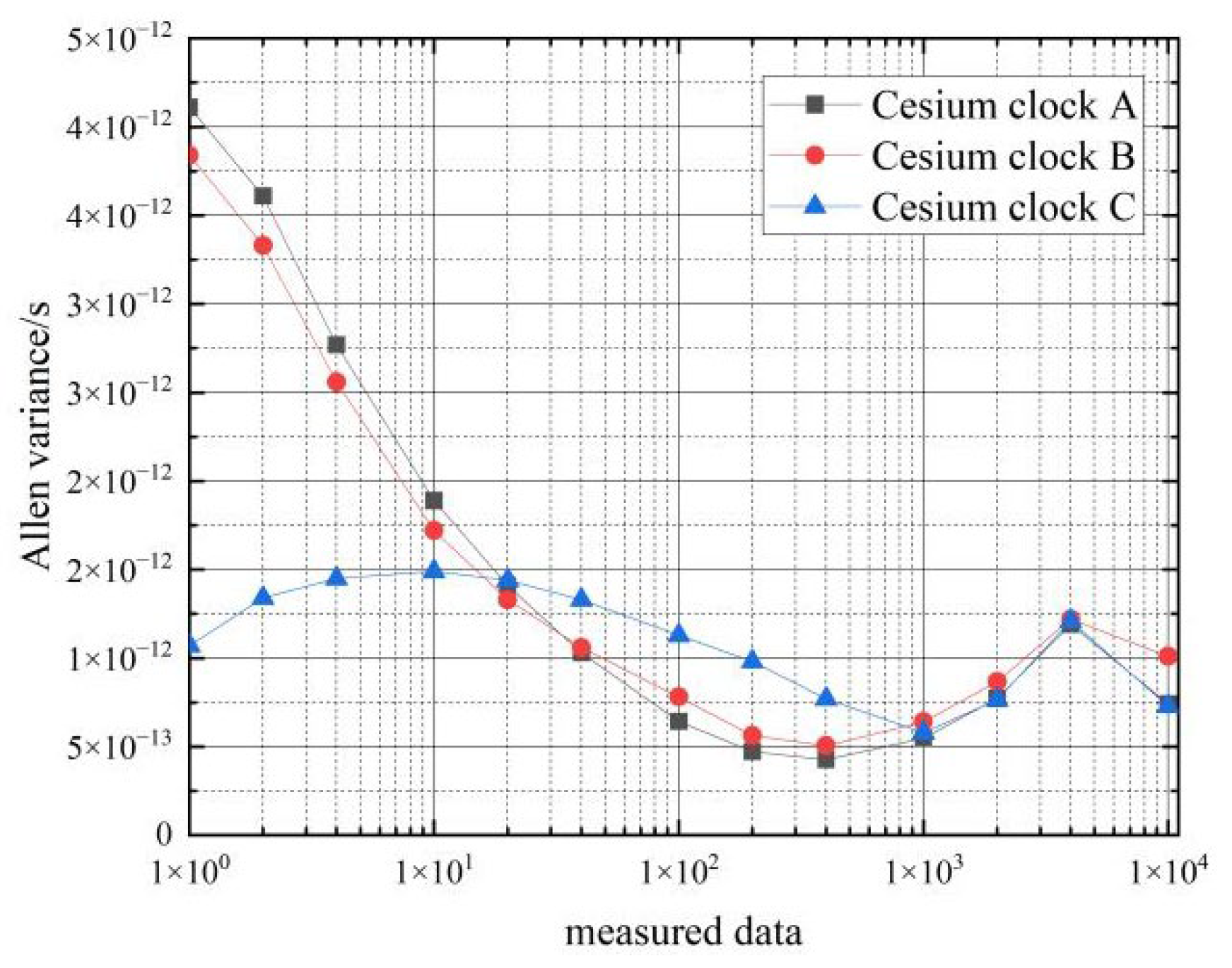
Figure 7.
Frequency stability of the car 1 cesium clocks at stationary state.
Figure 7.
Frequency stability of the car 1 cesium clocks at stationary state.
Figure 8.
Frequency stability of the car 2 cesium clocks at stationary state.
Figure 8.
Frequency stability of the car 2 cesium clocks at stationary state.
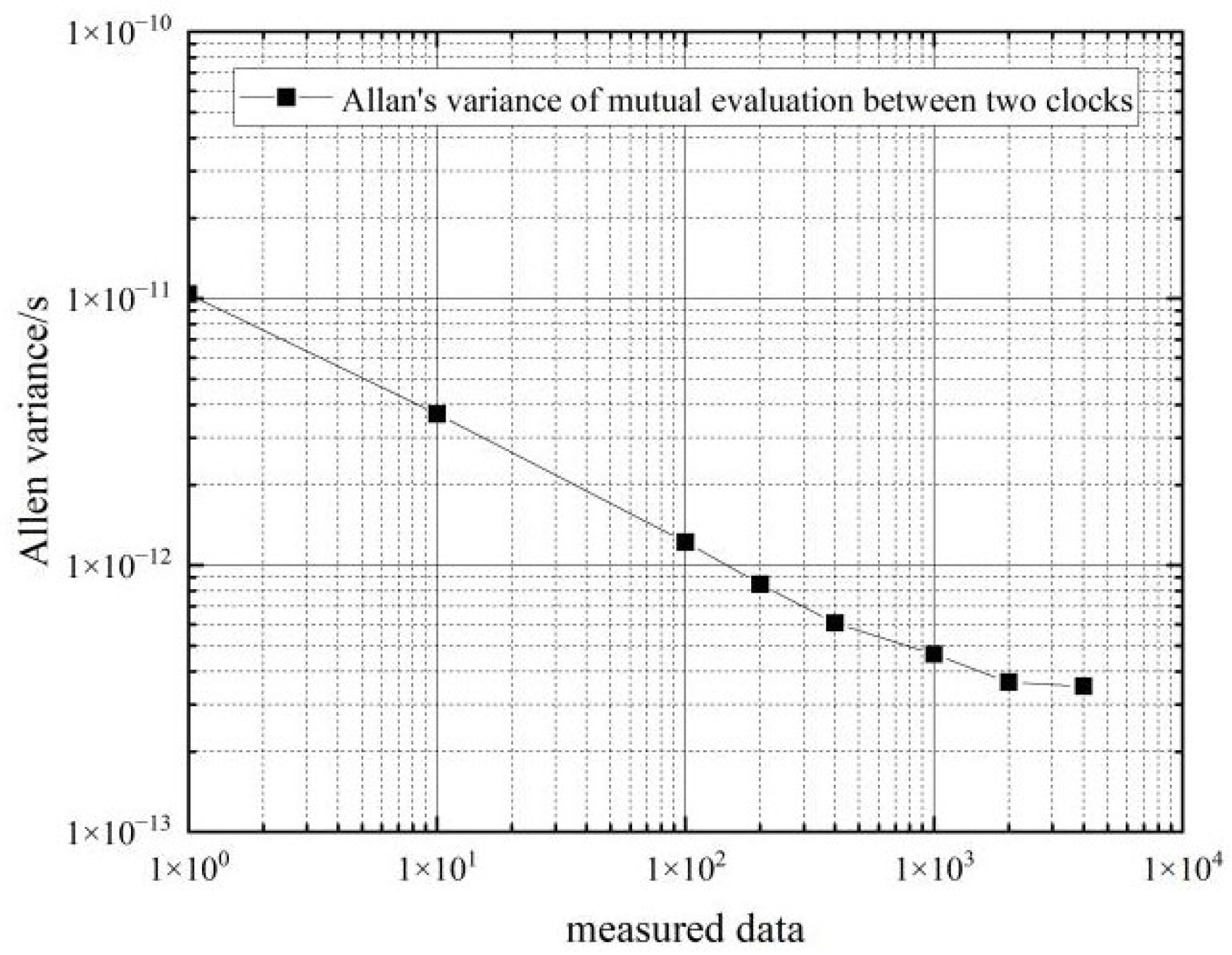
Figure 9.
Frequency stability of two hydrogen clocks in the moving state for mutual evaluation.
Figure 9.
Frequency stability of two hydrogen clocks in the moving state for mutual evaluation.
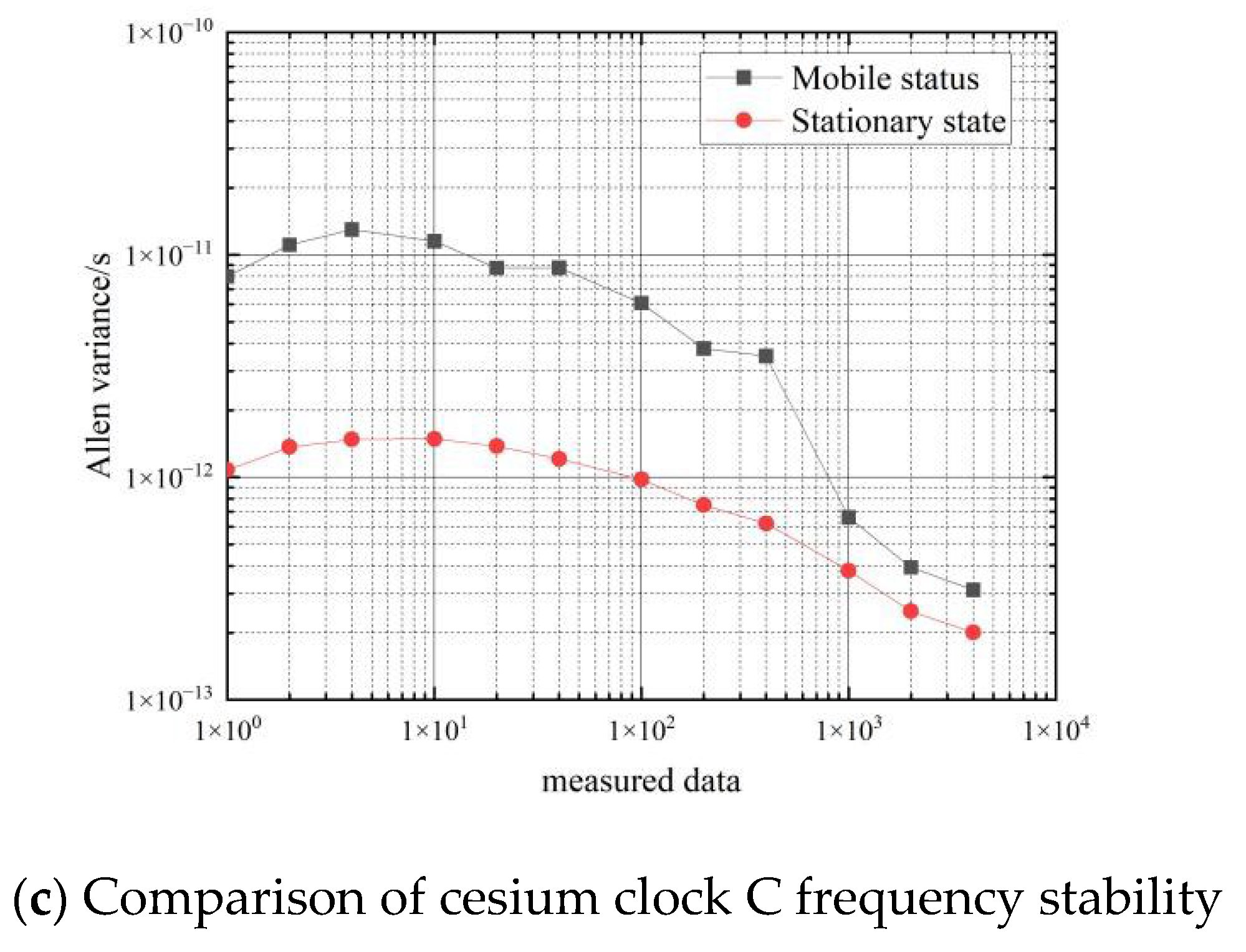
Figure 10.
Comparison of the frequency stability of a cesium clock at stationary and moving states.
Figure 10.
Comparison of the frequency stability of a cesium clock at stationary and moving states.
Figure 11.
Frequency stability of cesium clock moving state.
Figure 11.
Frequency stability of cesium clock moving state.
Figure 12.
Comparison of the frequency stability of cesium clocks at a stationary and moving state.
Figure 12.
Comparison of the frequency stability of cesium clocks at a stationary and moving state.
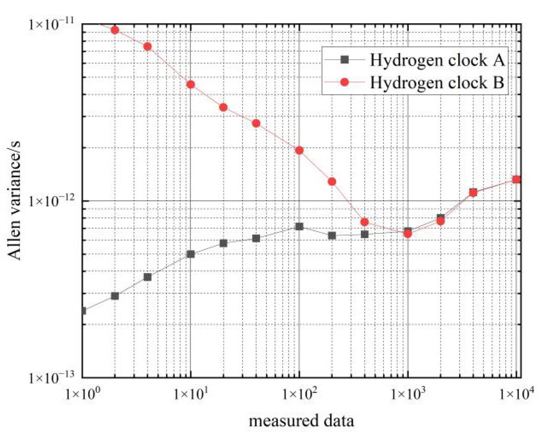
Figure 13.
Frequency stability during the recovery phase of hydrogen clocks.
Figure 13.
Frequency stability during the recovery phase of hydrogen clocks.
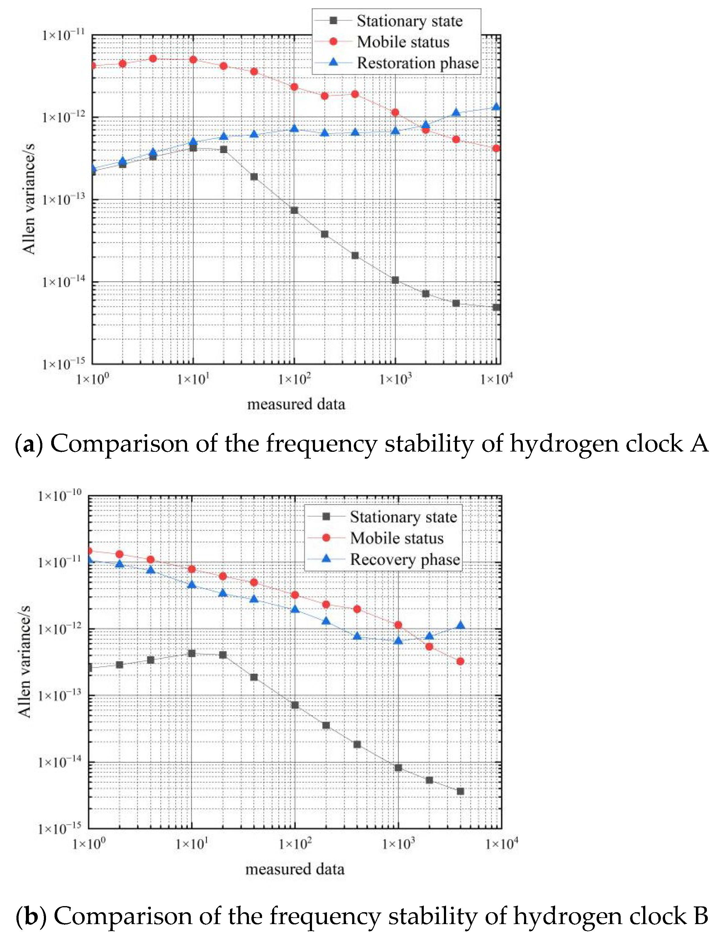
Figure 14.
Comparison of the frequency stability of three states of the hydrogen clock.
Figure 14.
Comparison of the frequency stability of three states of the hydrogen clock.
Figure 15.
Frequency stability during the recovery phase of cesium clocks.
Figure 15.
Frequency stability during the recovery phase of cesium clocks.
Figure 16.
Comparison of frequency stability in the three states of the cesium clock.
Figure 16.
Comparison of frequency stability in the three states of the cesium clock.
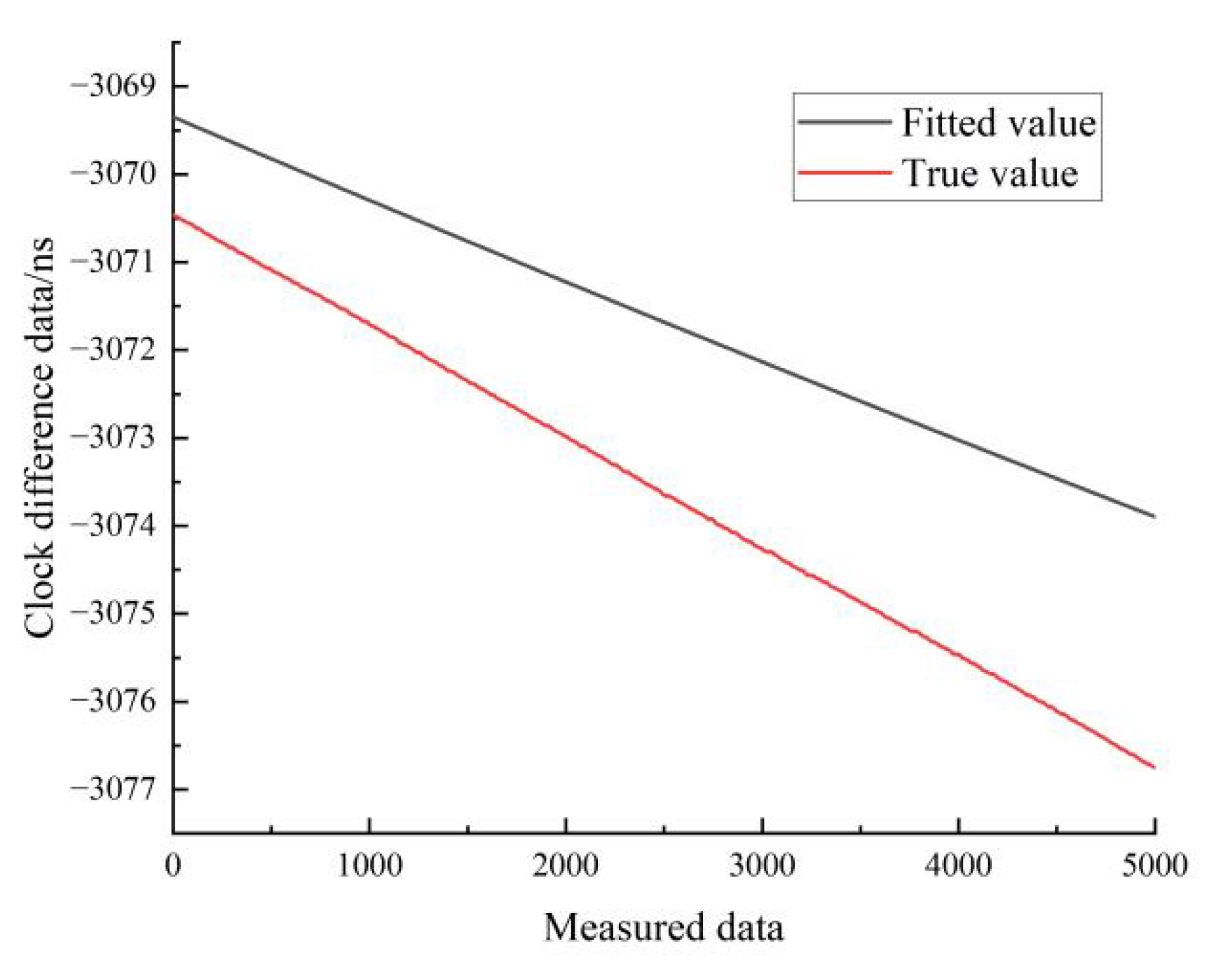
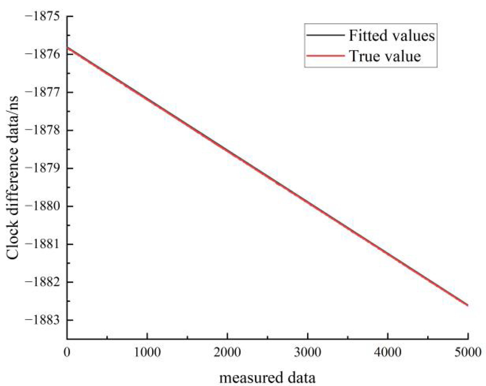
Figure 17.
Comparison of linear fitted and true values for hydrogen clock A at stationary state.
Figure 17.
Comparison of linear fitted and true values for hydrogen clock A at stationary state.
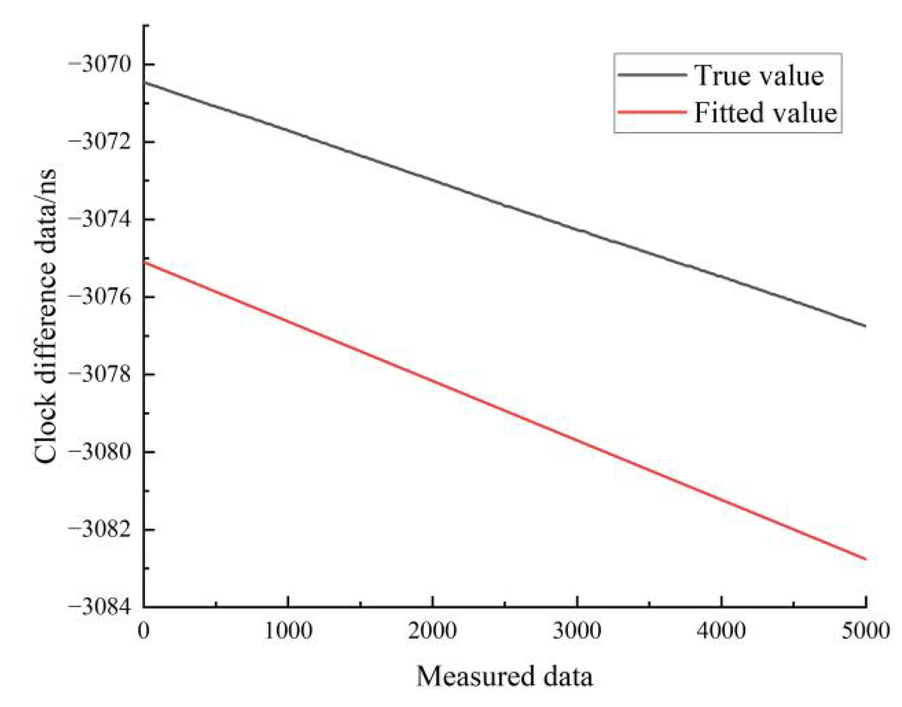
Figure 18.
Comparison of linear fitted and true values for the moving state of hydrogen clock A.
Figure 18.
Comparison of linear fitted and true values for the moving state of hydrogen clock A.
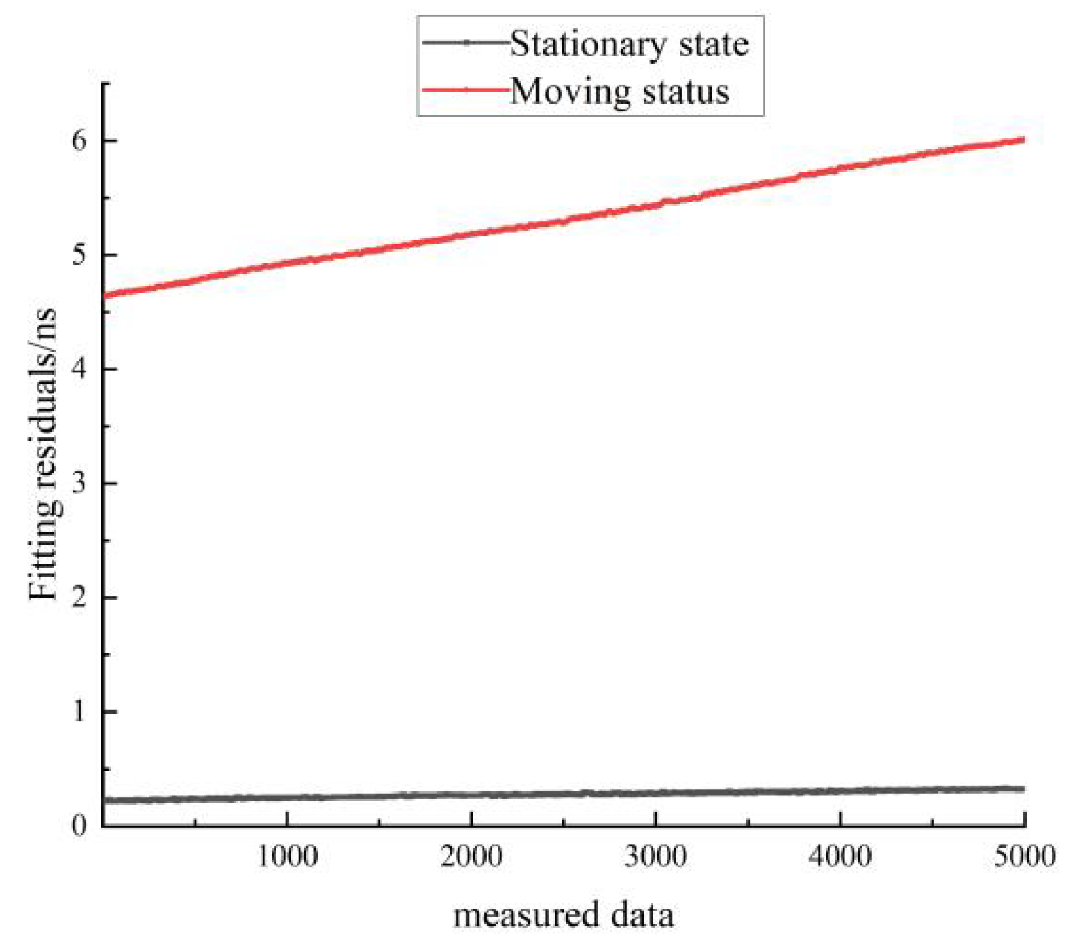
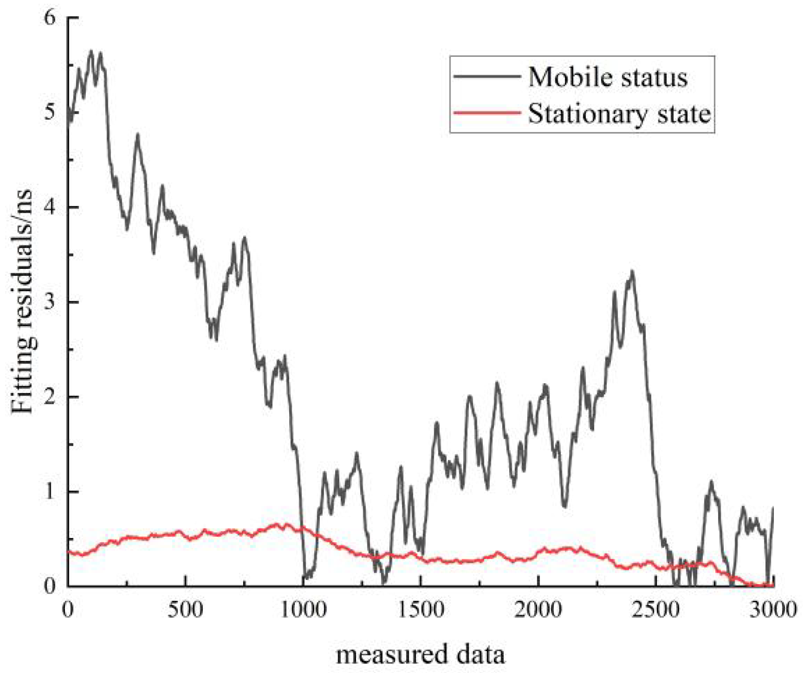
Figure 19.
Comparison of the residuals of the linear fit for the stationary and moving states of hydrogen clock A.
Figure 19.
Comparison of the residuals of the linear fit for the stationary and moving states of hydrogen clock A.
Figure 20.
Comparison between the quadratic fit and the true value of the hydrogen clock A at stationary state.
Figure 20.
Comparison between the quadratic fit and the true value of the hydrogen clock A at stationary state.
Figure 21.
Comparison of the quadratic fitted and true values for the moving state of hydrogen clock A.
Figure 21.
Comparison of the quadratic fitted and true values for the moving state of hydrogen clock A.
Figure 22.
Comparison of the residuals of the quadratic fit for the stationary and moving states of the hydrogen clock A.
Figure 22.
Comparison of the residuals of the quadratic fit for the stationary and moving states of the hydrogen clock A.
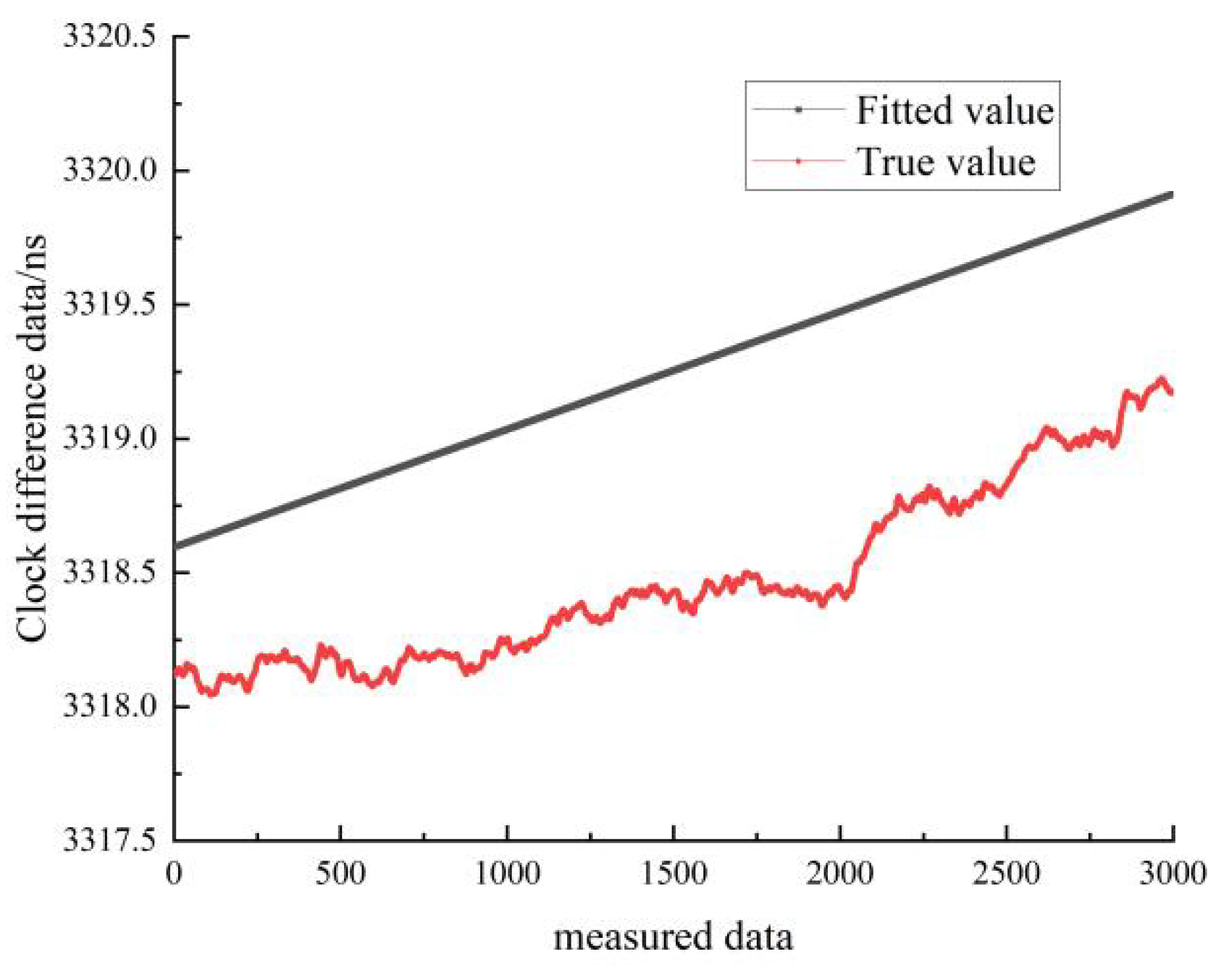
Figure 23.
Comparison of the linearly fitted and true values of cesium clock A in the stationary state.
Figure 23.
Comparison of the linearly fitted and true values of cesium clock A in the stationary state.
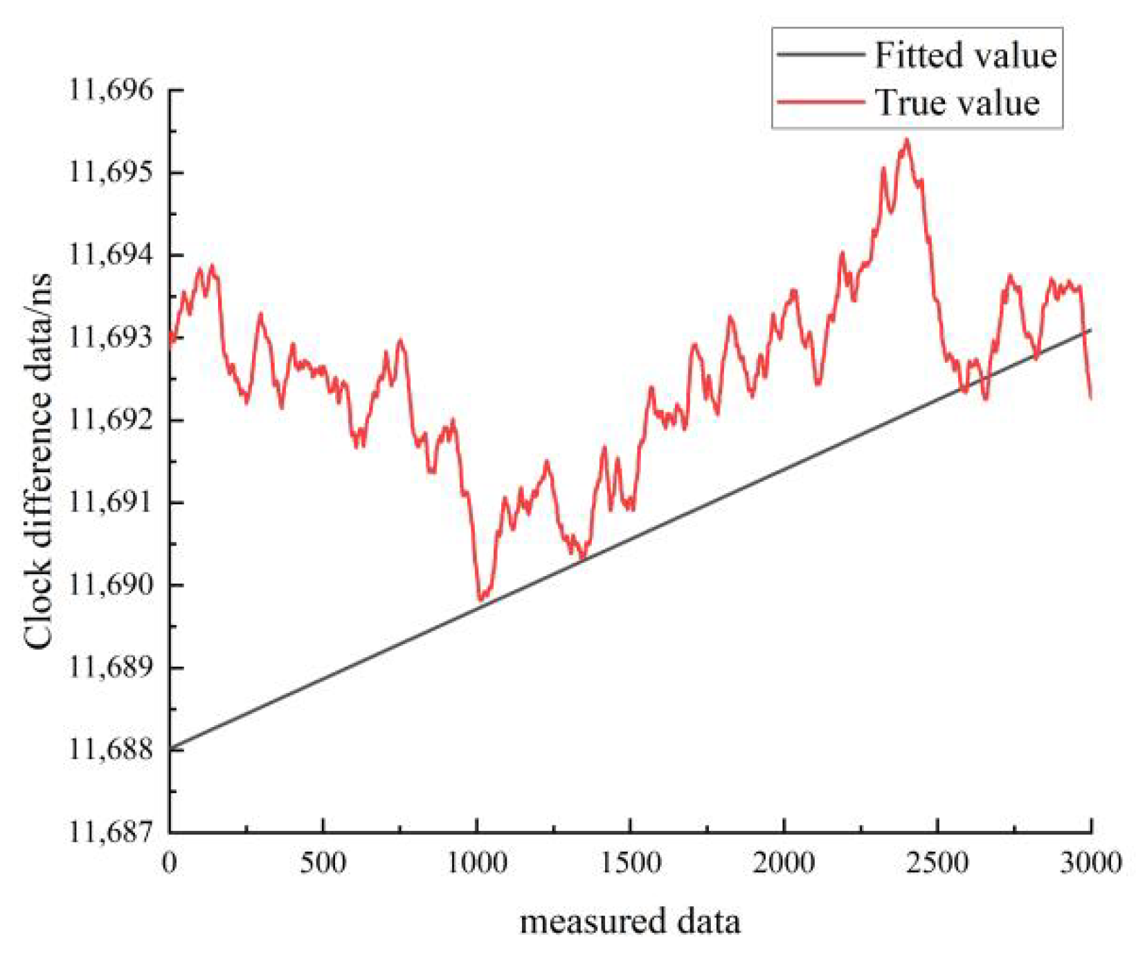
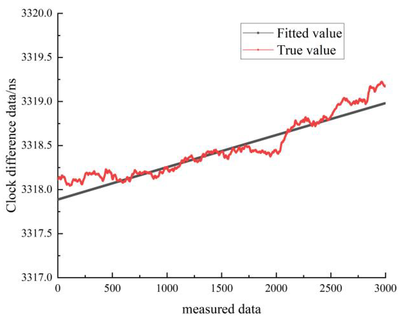
Figure 24.
Comparison of linear fitted and true values for the moving state of the cesium clock A.
Figure 24.
Comparison of linear fitted and true values for the moving state of the cesium clock A.
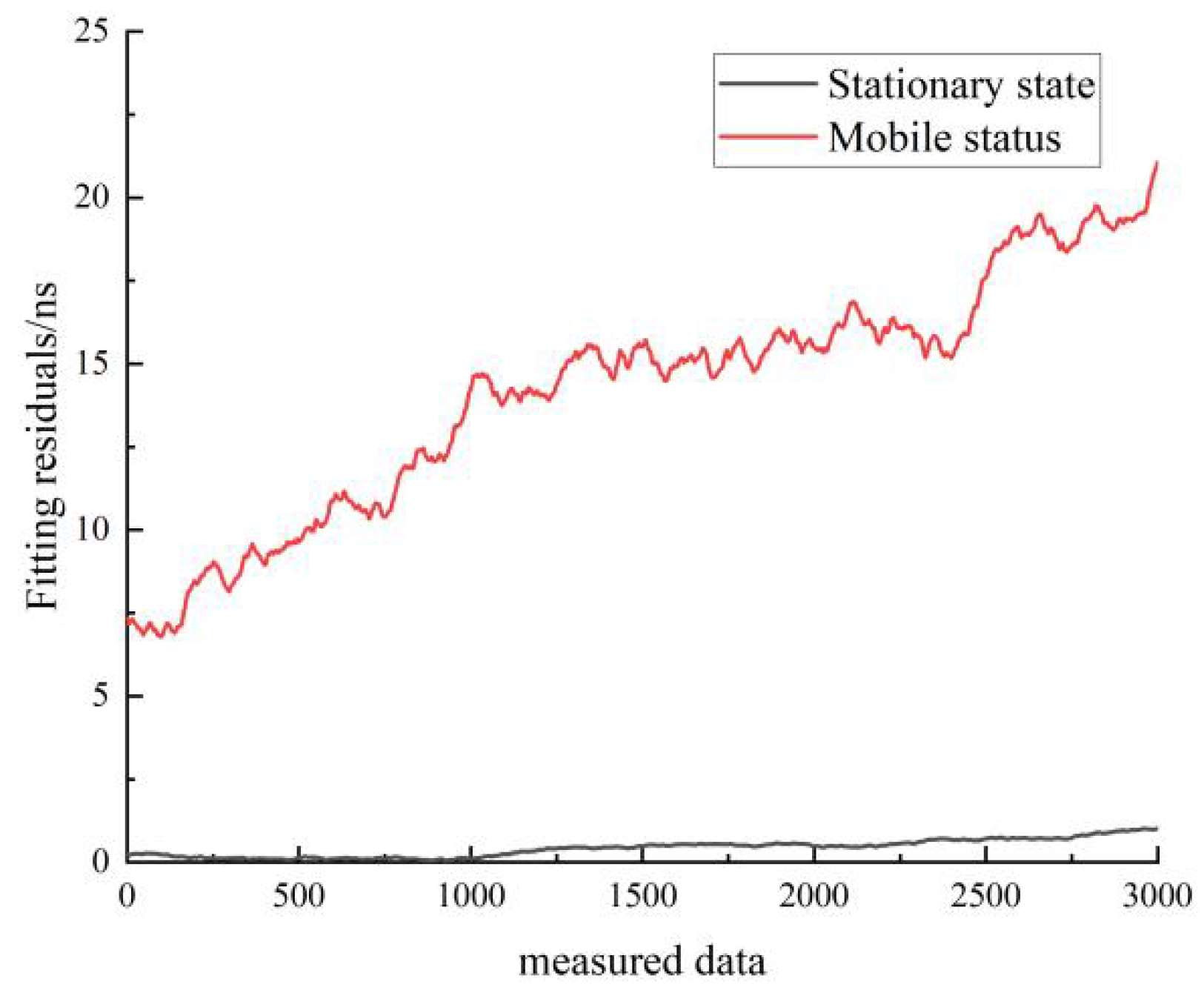
Figure 25.
Comparison of the residuals of the linear fit for the stationary and moving states of the cesium clock A.
Figure 25.
Comparison of the residuals of the linear fit for the stationary and moving states of the cesium clock A.
Figure 26.
Comparison between the quadratic fit and the true value of cesium clock A at stationary state.
Figure 26.
Comparison between the quadratic fit and the true value of cesium clock A at stationary state.
Figure 27.
Comparison of the quadratic fitted and true values for the moving state of cesium clock A.
Figure 27.
Comparison of the quadratic fitted and true values for the moving state of cesium clock A.
Figure 28.
Comparison of the residuals of the quadratic fit for the stationary and moving states of cesium clock A.
Figure 28.
Comparison of the residuals of the quadratic fit for the stationary and moving states of cesium clock A.
Table 1.
Nominal indexes of hydrogen atomic clock under static state.
Table 1.
Nominal indexes of hydrogen atomic clock under static state.
| Index Name | Index Requirements |
|---|
| Frequency stability of 1 s | ≤ |
| Frequency stability of 10 s | ≤ |
| Frequency stability of 100 s | ≤ |
| Frequency stability of 1000 s | ≤ |
| Frequency stability of 10,000 s | ≤ |
Table 2.
Calculations of frequency stability of hydrogen clocks at stationary state.
Table 2.
Calculations of frequency stability of hydrogen clocks at stationary state.
| Measured Data/s | Car 1 Hydrogen Clock Mutual Evaluation/s |
|---|
| 1 | |
| 10 | |
| 100 | |
| 1000 | |
| 10,000 | |
Table 3.
Calculated frequency stability of each cesium clock at stationary state.
Table 3.
Calculated frequency stability of each cesium clock at stationary state.
| Measured Data | Car 1 Cesium Clock A/s | Car 1 Cesium Clock B/s | Car 1 Cesium Clock C/s | Car 2 Cesium Clock A/s | Car 2 Cesium Clock B/s | Car 2 Cesium Clock C/s |
|---|
| 1 | | | | | | |
| 10 | | | | | | |
| 100 | | | | | | |
| 1000 | | | | | | |
| 10,000 | | | | | | |
Table 4.
Calculated frequency stability of the two hydrogen clocks in the moving state for mutual evaluation.
Table 4.
Calculated frequency stability of the two hydrogen clocks in the moving state for mutual evaluation.
| Measured Data/s | Allan’s Variance for the
Two Hydrogen Clocks Mutual Evaluation/s |
|---|
| 1 | |
| 10 | |
| 100 | |
| 200 | |
| 400 | |
| 1000 | |
| 2000 | |
| 4000 | |
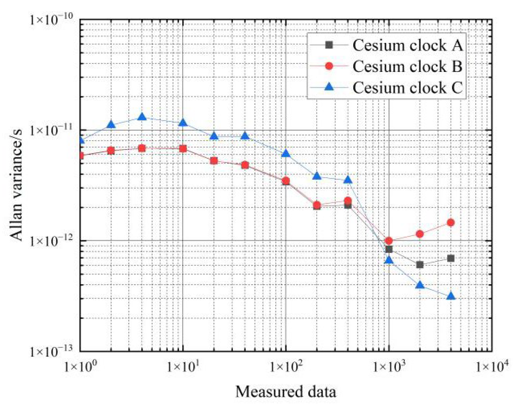
Table 5.
Calculated frequency stability of each cesium clock in the moving state.
Table 5.
Calculated frequency stability of each cesium clock in the moving state.
| Measured Data/s | Allan’s Variance of Cesium Clock A/s | Allan’s Variance of Cesium Clock B/s | Allan’s Variance of Cesium Clock C/s |
|---|
| 1 | | | |
| 10 | | | |
| 100 | | | |
| 1000 | | | |
| 4000 | | | |
Table 6.
Calculated frequency stability of each hydrogen clock in the recovery phase.
Table 6.
Calculated frequency stability of each hydrogen clock in the recovery phase.
| Measured Data/s | Allan’s Variance of Hydrogen Clock A/s | Allan’s Variance of Hydrogen Clock B/s |
|---|
| 1 | | |
| 10 | | |
| 100 | | |
| 1000 | | |
| 4000 | | |
Table 7.
Calculated frequency stability of each cesium clock during the conversion phase.
Table 7.
Calculated frequency stability of each cesium clock during the conversion phase.
| Measured Data/s | Allan’s Variance of Cesium Clock A/s | Allan’s Variance of Cesium Clock B/s | Allan’s Variance of Cesium Clock C/s |
|---|
| 1 | | | |
| 10 | | | |
| 100 | | | |
| 1000 | | | |
| 10,000 | | | |
Table 8.
Comparison of the three main types of noise in the stationary and moving states of the hydrogen atomic clock.
Table 8.
Comparison of the three main types of noise in the stationary and moving states of the hydrogen atomic clock.
| | WFM/s | RWFM/s | WPM/s |
|---|
| Hydrogen clock A at stationary state | | | |
| Hydrogen clock A in mobile state | | | |
| Hydrogen clock B at stationary state | | | |
| Hydrogen clock B in mobile state | | | |
Table 9.
Comparison of the three main types of noise in the stationary and moving states of a cesium atomic clock.
Table 9.
Comparison of the three main types of noise in the stationary and moving states of a cesium atomic clock.
| | WFM/s | RWFM/s | WPM/s |
|---|
| cesium clock A at stationary state | | | |
| cesium clock A in mobile state | | | |
| cesium clock B at stationary state | | | |
| cesium clock B in mobile state | | | |
Table 10.
Residuals and RMS of linear and quadratic fits for stationary and moving states.
Table 10.
Residuals and RMS of linear and quadratic fits for stationary and moving states.
| | Stationary State Linear Fit | Stationary State Quadratic Fit | Moving State Linear Fit | Moving State Quadratic Fit |
|---|
| RMS | 0.2801 | 0.02819 | 5.3366 | 2.0098 |
| Fitting residuals/ns | 0.2787 | 0.0276 | 5.3218 | 1.9463 |
Table 11.
Residuals and RMS for linear and quadratic fits to the cesium clock at stationary and moving states.
Table 11.
Residuals and RMS for linear and quadratic fits to the cesium clock at stationary and moving states.
| | Stationary State Linear Fit | Stationary State Quadratic Fit | Moving State Linear Fit | Moving State Quadratic Fit |
|---|
| RMS | 0.7938 | 0.1107 | 4.0616 | 45.6283 |
| Fitting residuals | 0.7837 | 0.1346 | 3.5940 | 44.8563 |


