Stepped Coastal Water Warming Revealed by Multiparametric Monitoring at NW Mediterranean Fixed Stations †

 ,
,  , , ,
, , ,
Abstract
1. Introduction
2. Materials and Methods
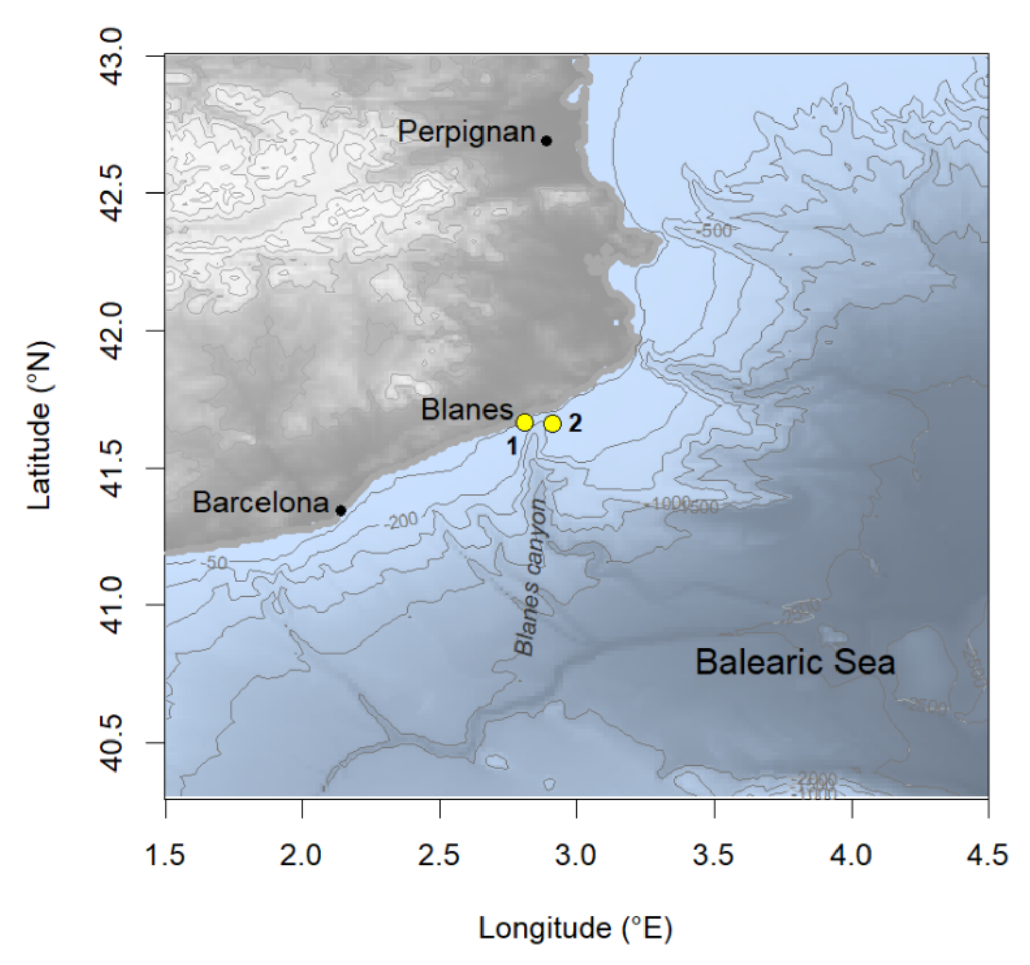
2.1. In Situ Data
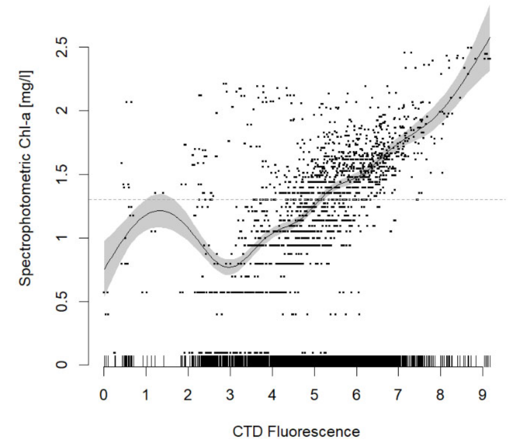
2.2. Derived Variables and Auxiliary Data
3. Results
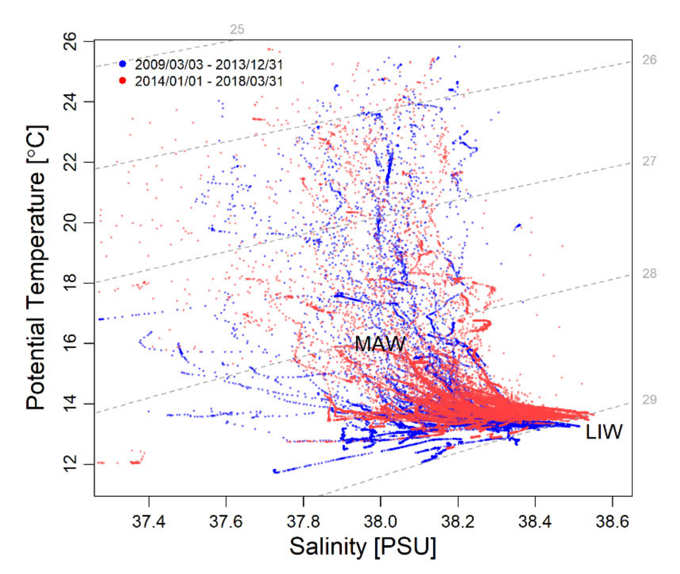
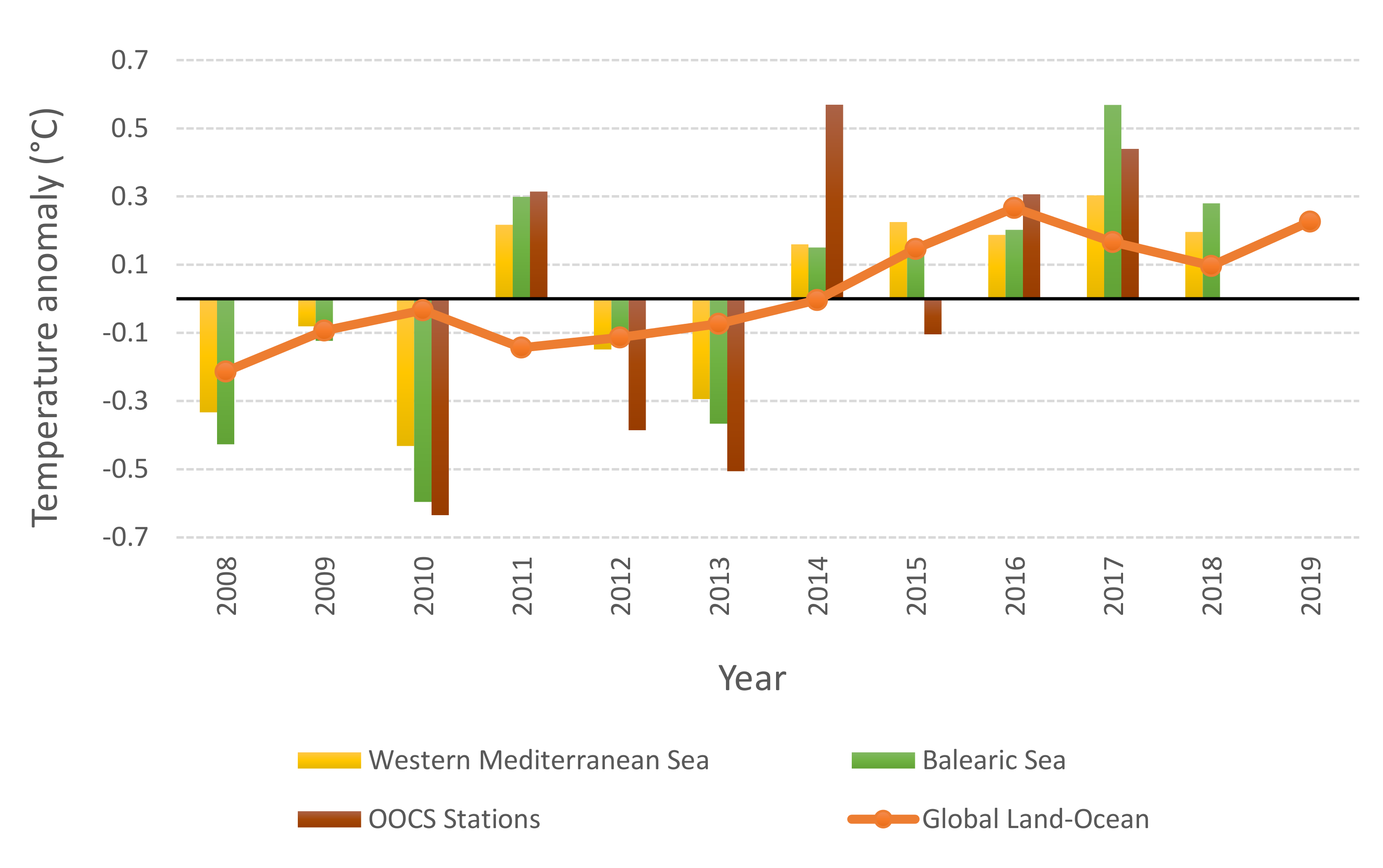
3.1. Water Temperature and Salinity
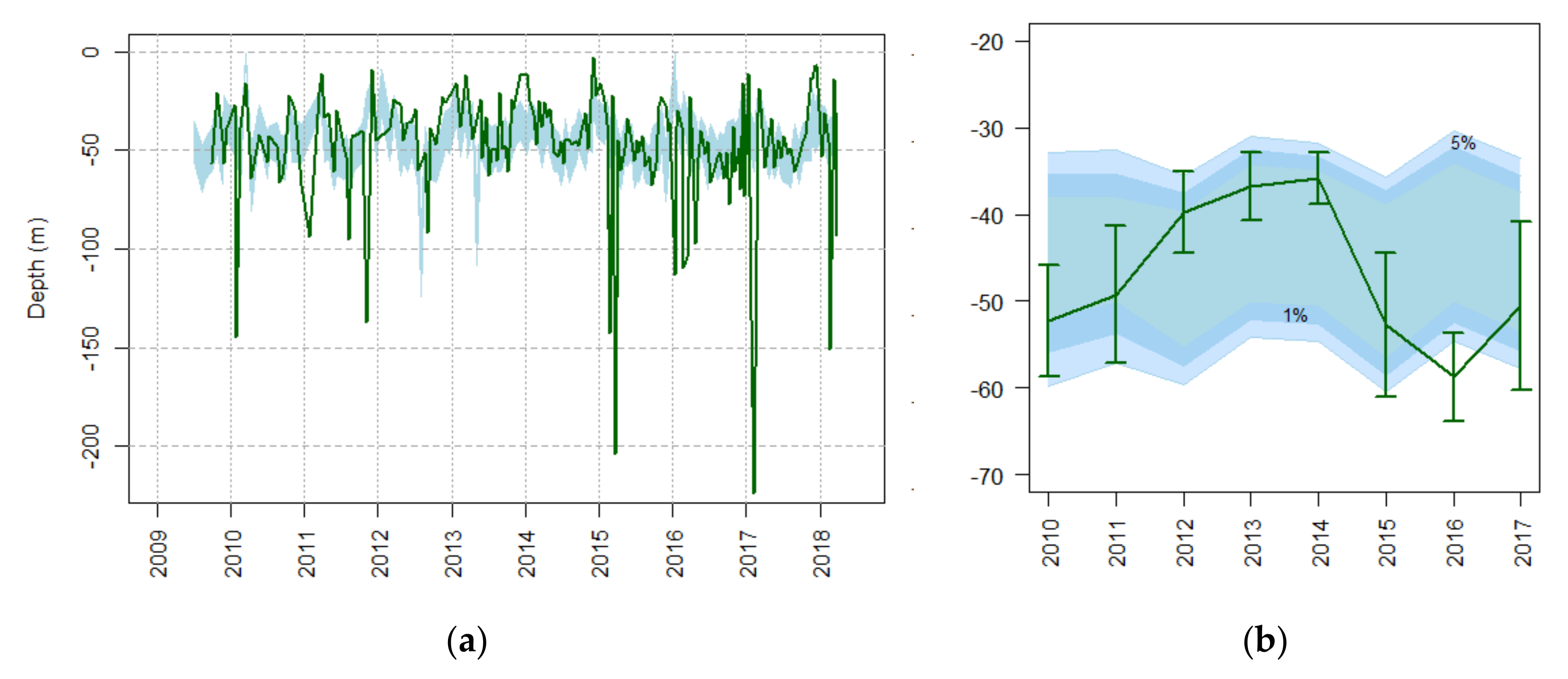
3.2. Mixed Layer Depth (MLD)
3.3. Biogeochemical Water Properties
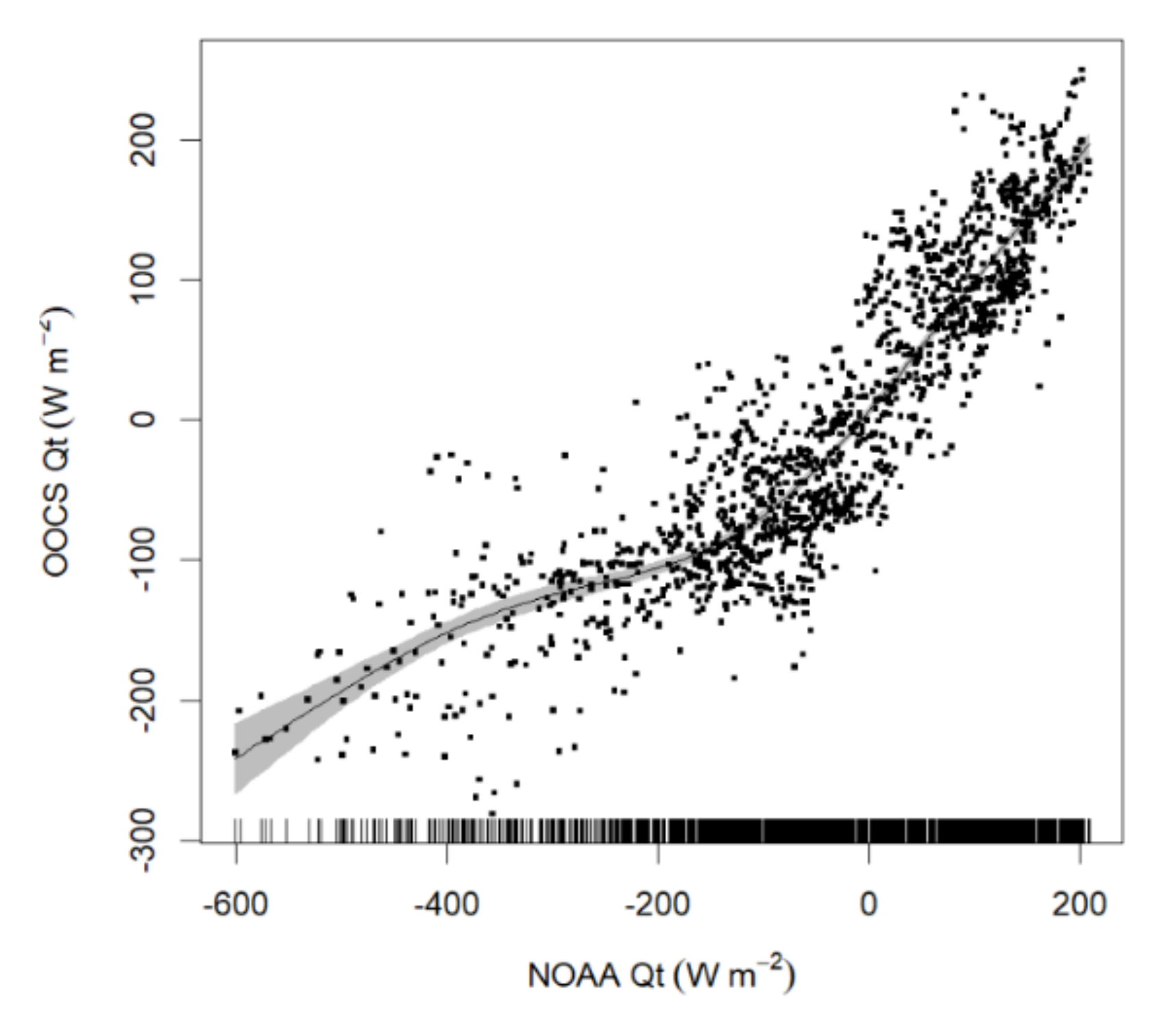
3.4. Air-Sea Heat Fluxes
4. Discussion
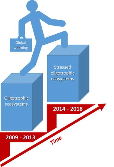
5. Conclusions
Supplementary Materials
Author Contributions
Funding
Acknowledgments
Conflicts of Interest
Appendix A
References
- Cheng, L.; Abraham, J.; Husfather, Z.; Trenberth, K.E. How fast are the oceans warming? Science 2019, 363, 128–129. [Google Scholar] [CrossRef] [PubMed]
- NOAA National Centers for Environmental Information. State of the Climate: Global Climate Report for Annual 2019; NOAA National Centers for Environmental Information: Asheville, NC, USA, 2020. Available online: https://www.ncdc.noaa.gov/sotc/global/201913 (accessed on 14 March 2020).
- WMO,2019. The Global Climate in 2015–2019. Weather Climate Water. World Meteorological Organization. 21pp. Available online: https://library.wmo.int/doc_num.php?explnum_id=9936 (accessed on 5 April 2020).
- Yin, J.; Overpeck, J.; Peyser, C.; Stouffer, R. Big jump of record warm global mean surface temperature in 2014–2016 related to unusually large oceanic heat releases. Geophys. Res. Lett. 2018, 45, 1069–1078. [Google Scholar] [CrossRef]
- NOAA. Available online: https://www.noaa.gov/news/2019-was-2nd-hottest-year-on-record-for-earth-say-noaa-nasa (accessed on 5 April 2020).
- Borghini, M.; Bryden, H.; Schroeder, K.; Sparnocchia, S.; Vetrano, A. The Mediterranean is becoming saltier. Ocean Sci. 2014, 10, 693–700. [Google Scholar] [CrossRef]
- Schroeder, K.; Chiggiato, J.; Bryden, H.L.; Borghini, M.; Ben Ismail, S. Abrupt climate shift in the Western Mediterranean Sea. Sci. Rep. 2016, 6, 23009. [Google Scholar] [CrossRef]
- Coma, R.; Ribes, M.; Serrano, E.; Jimenez, E.; Salat, J.; Pascual, J. Global warming-enhanced stratification and mass mortality event in the Mediterranean. Proc. Natl. Acad. Sci. USA 2009, 106, 6176–6181. [Google Scholar] [CrossRef]
- Rivetti, I.; Fraschetti, S.; Lionello, P.; Zambianchi, E.; Boero, F. Global Warming and Mass Mortalities of Benthic Invertebrates in the Mediterranean Sea. PLoS ONE 2014, 9, e115655. [Google Scholar] [CrossRef]
- Garrabou, J.; Coma, R.; Bensoussan, N.; Bally, M.; Chevaldonné, P.; Cigliano, M.; Diaz, D.; Harmelin, J.G.; Gambi, M.C.; Kersting, D.K.; et al. Mass mortality in Northwestern Mediterranean rocky benthic communities: Effects of the 2003 heat wave. Glob. Change Biol. 2009, 15, 1090–1103. [Google Scholar] [CrossRef]
- Huete-Stauffer, C.; Vielmini, I.; Palma, M.; Navone, A.; Panzalis, P.; Vezzulli, L.; Misic, C.; Cerrano, C. Paramuricea clavata (Anthozoa, Octocorallia) loss in the Marine Protected Area of Tavolara (Sardinia, Italy) due to a mass mortality event. Mar. Ecol. 2011, 32, 107–116. [Google Scholar] [CrossRef]
- Vázquez-Luis, M.; Álvarez, E.; Barrajón, A.; García-March, J.R.; Grau, A.; Hendriks, I.E.; Jiménez, S.; Kersting, D.; Moreno, D.; Pérez, M.; et al. Pinna nobilis: A Mass Mortality Event in Western Mediterranean Sea. Front. Mar. Sci. 2017, 4. [Google Scholar] [CrossRef]
- Bensoussana, N.; Romano, J.-C.; Harmelin, J.-G.; Garrabou, J. High resolution characterization of northwest Mediterranean coastal waters thermal regimes: To better understand responses of benthic communities to climate change. Estuar. Coast. Shelf Sci. 2010, 87, 431–441. [Google Scholar] [CrossRef]
- Williamson, P.; Smythe-Wright, D.; Burkill, P. Future of the Ocean and Its Seas: A Non-Governmental Scientific Perspective on Seven Marine Research Issues of G7 Interest ICSU-IAPSO-IUGGSCOR; IUGG: Paris, France, 2016. [Google Scholar]
- Di Camillo, C.G.; Cerrano, C. Mass Mortality Events in the NW Adriatic Sea: Phase Shift from Slow- to Fast-Growing Organisms. PLoS ONE 2015, 10, e0126689. [Google Scholar] [CrossRef] [PubMed]
- Cebrian, E.; Uriz, M.J.; Garrabou, J.; Ballesteros, E. Sponge Mass Mortalities in a Warming Mediterranean Sea: Are Cyanobacteria-Harboring Species Worse Off? PLoS ONE 2011, 6, e20211. [Google Scholar] [CrossRef] [PubMed]
- Rivetti, I.; Boero, F.; Fraschetti, S.; Zambianchi, E.; Lionello, P. Anomalies of the upper water column in the Mediterranean Sea. Global Planet. Change 2017, 151, 68–79. [Google Scholar] [CrossRef]
- Polovina, J.; Howell, E.A.; Abecassis, M. Ocean’s least productive waters are expanding. Geophys. Res. Lett. 2008, 35, L03618. [Google Scholar] [CrossRef]
- Steinacher, M.; Joos, F.; Frölicher, T.L.; Bopp, L.; Cadule, P.; Cocco, V.; Doney, S.C.; Gehlen, M.; Lindsay, K.; Moore, J.K.; et al. Projected 21st century decrease in marine productivity: A multi-model analysis. Biogeosciences 2010, 7, 979–1005. [Google Scholar] [CrossRef]
- Gittings, J.A.; Raitsos, D.E.; Krokos, G.; Hoteit, I. Impacts of warming on phytoplankton abundance and phenology in a typical tropical marine ecosystem. Sci. Rep. 2018, 8. [Google Scholar] [CrossRef]
- Danovaro, R.; Aguzzi, J.; Fanelli, E.; Billet, D.; Gjerde, K.; Jamieson, A.; Ramirez-Llodra, E.; Smith, C.R.; Snelgrove, P.V.R.; Thomsen, L.; et al. A new international ecosystem-based strategy for the global deep ocean. Science 2017, 355, 452–454. [Google Scholar] [CrossRef]
- Thomsen, L.; Aguzzi, J.; Costa, C.; De Leo, F.; Ogston, A.; Purser, A. The oceanic biological pump: Rapid carbon transfer to the Deep Sea during winter. Sci. Rep. 2017, 7, 10763. [Google Scholar] [CrossRef]
- Aguzzi, J.; Chatzievangelou, D.; Marini, S.; Fanelli, E.; Danovaro, R.; Flögel, S.; Lebris, N.; Juanes, F.; De Leo, F.; Del Rio, J.; et al. New high-tech interactive and flexible networks for the future monitoring of deep-sea ecosystems. Environ. Sci. Technol. 2019, 53, 6616–6631. [Google Scholar] [CrossRef]
- Danovaro, R.; Fanelli, E.; Aguzzi, J.; Billett, D.; Carugati, L.; Corinaldesi, C.; Dell’Anno, A.; Gjerde, K.; Jamieson, A.J.; Kark, S.; et al. Ecological indicators for an integrated global deep-ocean strategy. Nat. Ecol. Evol. 2019, (in press).
- Rountree, R.; Aguzzi, J.; Marini, S.; Fanelli, E.; De Leo, C.F.; Del Rio, J.; Juanes, F. Towards an optimal design for ecosystem-level ocean observatories. Oceanogr. Mar. Biol. Ann. Rev. (OMBAR) 2020, 50. (in press).
- Cristini, L.; Lampitt, R.S.; Cardin, V.; Delory, E.; Haugan, P.; O’Neill, N.; Petihakis, G.; Ruhl, H.A. Cost and value of multidisciplinary fixed-point ocean observatories. Marine Policy 2016, 71, 138–146. [Google Scholar] [CrossRef]
- Marty, J.C.; Chiavérini, J. Hydrological changes in the Ligurian Sea (NW Mediterranean, DYFAMED site) during 1995–2007 and biogeochemical consequences. Biogeosciences 2010, 7, 2117–2128. [Google Scholar] [CrossRef]
- Bahamon, N.; Aguzzi, J.; Bernardello, R.; Ahumada-Sempoal, M.-A.; Puigdefabregas, J.; Cateura, J.; Muñoz, E.; Velásquez, Z.; Cruzado, A. The new pelagic Operational Observatory of the Catalan Sea (OOCS) for the multisensor coordinated measurement of atmospheric and oceanographic conditions. Sensors 2011, 11, 11251–11272. [Google Scholar] [CrossRef] [PubMed]
- Aguzzi, J.; Chatzievangelou, D.; Francescangeli, M.; Marini, S.; Bonofiglio, F.; del Río, J.; Danovaro, R. The hierarchic treatment of marine ecological information from spatial networks of benthic platforms. Sensors 2020, 20, 1751. [Google Scholar] [CrossRef] [PubMed]
- Hansen, H.P.; Koroleff, F. Determination of nutrients. In Methods of Seawater Analysis; Grasshof, K., Ed.; Wiley: Hoboken, NJ, USA, 1999; pp. 159–228. [Google Scholar]
- Jeffrey, S.W.; Humphrey, G.F. New Spectrophotometric Equations for Determining Chlorophylls a, b, c and c2 in Higher Plants, Algae and Natural Phytoplankton. Biochem. Physiol. Pflanz. 1975, 167, 191–194. [Google Scholar] [CrossRef]
- Kim, Y.-J.; Gu, C. Smoothing spline Gaussian regression: More scalable computation via efficient approximation. J. R. Stat. Soc. B 2004, 66, 337–356. [Google Scholar] [CrossRef]
- Acker, J.G.; Leptoukh, G. Online Analysis Enhances Use of NASA Earth Science Data, Eos, Trans; AGU: Hoboken, NJ, USA, 2007; Volume 88, pp. 14–17. [Google Scholar]
- De Boyer Montegut, C.; Madec, G.; Fisher, A.S.; Lazar, A.; Iudicone, D. Mixed layer depth over the global ocean: An examination of profile data and a profile-based climatology. J. Geophys. Res. 2004, 109, C12003. [Google Scholar] [CrossRef]
- Weller, R.A.; Plueddemnn, A.J. Observations of the vertical structure of the oceanic boundary layer. J. Geophys. Res. 1996, 101, 8789–8806. [Google Scholar] [CrossRef]
- NOAA. Available online: http://iridl.ldeo.columbia.edu/SOURCES/.NOAA/.NCEP-NCAR/.CDAS-1/.DAILY/ (accessed on 1 March 2020).
- Kalnay, E.; Kanamitsu, M.; Kistler, R.; Collins, W.; Deaven, D.; Gandin, L.; Iredell, M.; Saha, S.; White, G.; Woollen, J.; et al. The NCEP/NCAR 40-Year Reanalysis Project. Bull. Am. Meteorol. Soc. 1996, 77, 437–472. [Google Scholar] [CrossRef]
- Houpert, L.; Durrieu de Madron, X.; Testor, P.; Bosse, A.; D’Otertenzio, F.; Bouin, M.M.; Dausse, D.; Le Goff, H.; Kunesch, S.; Labaste, M.; et al. Observations of open-ocean deep convection in the northwestern Mediterranean Sea: Seasonal and interannual variability of mixing and deep water masses for the 2007-2013 Period. J. Geophys. Res. Oceans 2016, 121, 8139–8171. [Google Scholar] [CrossRef]
- Grignon, L.; Smeed, D.A.; Bryden, H.L.; Schroeder, K. Importance of the variability of hydrographic preconditioning for deep convection in the Gulf of Lion, NW Mediterranean. Ocean Sci. 2010, 6, 573–586. [Google Scholar] [CrossRef]
- Signorini, S.R.; Franz, B.A.; McClain, C.R. Chlorophyll variability in the oligotrophic gyres: Mechanisms, seasonality and trends. Front. Mar. Sci. 2015, 2, 1. [Google Scholar] [CrossRef]
- Valdés, L.; Peterson, W.; Church, K.; Marcos, M. Our changing oceans: Conclusions of the first International Symposium on the Effects of climate change on the world’s oceans. ICES J. Mar. Sci. 2009, 66, 1435–1438. [Google Scholar] [CrossRef][Green Version]
- Bernardello, R.; Cardoso, J.G.; Bahamon, N.; Donis, D.; Marinov, I.; Cruzado, A. Modelled interannual variability of vertical organic matter export related to phytoplankton bloom dynamics—A case-study for the NW Mediterranean Sea. Biogeosciences 2012, 9, 4233–4245. [Google Scholar] [CrossRef]
- Bahamon, N.; Cruzado, A. Modelling nitrogen fluxes in oligotrophic marine environments: NW Mediterranean Sea and NE Atlantic. Ecol. Model. 2003, 163, 223–244. [Google Scholar] [CrossRef]
- Gallisai, R.; Peters, F.; Volpe, G.; Basart, S.; Baldasano, J.M. Saharian dust deposition may affect phytoplankton growth in the Mediterranean Sea at ecological time scales. PLoS ONE 2014, 9, e110762. [Google Scholar] [CrossRef]
- Leyba, I.M.; Solman, S.A.; Saraceno, M. Trends in sea surface temperature and air-sea heat fluxes over the South Atlantic Ocean. Clim. Dyn. 2019. [Google Scholar] [CrossRef]
- Ahumada-Sempoal, M.A.; Flexas, M.M.; Bernardello, R.; Bahamon, N.; Cruzado, A. Northern Current variability ant its impact on the Blanes Canyon circulation: A numerical study. Prog. Oceanogr. 2013, 118, 61–70. [Google Scholar] [CrossRef]
- Song, K.; Yu, L. Air-sea heat flux climatologies in the Mediterranean Sea: Surface energy balance and its consistency with ocean heat storage. J. Geophys. Res. Oceans 2017, 122, 4068–4087. [Google Scholar] [CrossRef]
- Reed, R.K. On Estimating Insolation over the Ocean. J. Phys. Ocean. 1977, 7, 482–485. [Google Scholar] [CrossRef]
- Dobson, F.W.; Smith, S.D. Bulk models of solar radiation at sea. Q. J. R. Meteorol. Soc. 1988, 114, 165–182. [Google Scholar] [CrossRef]
- Seckel, G.R.; Beaudry, F.H. The radiation from sun and sky over the North Pacific Ocean (abstract). Trans. Am. Geophys. Union 1973, 54, 1114. [Google Scholar]
- Bunker, A.F. Computations of Surface Energy Flux and Annual Air–Sea Interaction Cycles of the North Atlantic Ocean. Mon. Weather Rev. 1976, 104, 1122–1140. [Google Scholar] [CrossRef]
- Garrett, C.; Outerbridge, R.; Thompson, K. Interannual variability in meterrancan heat and buoyancy fluxes. J. Clim. 1993, 6, 900–910. [Google Scholar] [CrossRef]
- Smith, S.D. Coefficients for sea surface wind stress, heat flux, and wind profiles as a function of wind speed and temperature. J. Geophys. Res. 1988, 93, 15467. [Google Scholar] [CrossRef]


| Deployment Number | Initial Date | Final Date | Days per Deployment | Days Between Deployments |
|---|---|---|---|---|
| 1 | 15/09/2009 | 08/02/2010 | 146 | - |
| 2 | 15/04/2010 | 28/04/2010 | 13 | 66 |
| 3 | 03/08/2010 | 19/01/2011 | 169 | 97 |
| 4 | 25/03/2011 | 03/06/2011 | 70 | 65 |
| 5 | 28/06/2011 | 04/10/2011 | 98 | 25 |
| 6 | 25/11/2011 | 25/05/2012 | 182 | 52 |
| 7 | 22/09/2012 | 29/12/2012 | 98 | 120 |
| 8 | 07/05/2013 | 31/05/2013 | 24 | 129 |
| 9 | 25/10/2013 | 28/05/2014 | 215 | 147 |
| 10 | 05/08/2014 | 22/09/2014 | 48 | 69 |
| 11 | 27/11/2014 | 10/12/2014 | 13 | 66 |
| 12 | 23/06/2015 | 07/09/2016 | 442 | 195 |
| 13 | 03/10/2016 | 20/12/2016 | 78 | 26 |
© 2020 by the authors. Licensee MDPI, Basel, Switzerland. This article is an open access article distributed under the terms and conditions of the Creative Commons Attribution (CC BY) license (http://creativecommons.org/licenses/by/4.0/).
Share and Cite
Bahamon, N.; Aguzzi, J.; Ahumada-Sempoal, M.Á.; Bernardello, R.; Reuschel, C.; Company, J.B.; Peters, F.; Gordoa, A.; Navarro, J.; Velásquez, Z.; et al. Stepped Coastal Water Warming Revealed by Multiparametric Monitoring at NW Mediterranean Fixed Stations. Sensors 2020, 20, 2658. https://doi.org/10.3390/s20092658
Bahamon N, Aguzzi J, Ahumada-Sempoal MÁ, Bernardello R, Reuschel C, Company JB, Peters F, Gordoa A, Navarro J, Velásquez Z, et al. Stepped Coastal Water Warming Revealed by Multiparametric Monitoring at NW Mediterranean Fixed Stations. Sensors. 2020; 20(9):2658. https://doi.org/10.3390/s20092658
Chicago/Turabian StyleBahamon, Nixon, Jacopo Aguzzi, Miguel Ángel Ahumada-Sempoal, Raffaele Bernardello, Charlotte Reuschel, Joan Baptista Company, Francesc Peters, Ana Gordoa, Joan Navarro, Zoila Velásquez, and et al. 2020. "Stepped Coastal Water Warming Revealed by Multiparametric Monitoring at NW Mediterranean Fixed Stations" Sensors 20, no. 9: 2658. https://doi.org/10.3390/s20092658
APA StyleBahamon, N., Aguzzi, J., Ahumada-Sempoal, M. Á., Bernardello, R., Reuschel, C., Company, J. B., Peters, F., Gordoa, A., Navarro, J., Velásquez, Z., & Cruzado, A. (2020). Stepped Coastal Water Warming Revealed by Multiparametric Monitoring at NW Mediterranean Fixed Stations. Sensors, 20(9), 2658. https://doi.org/10.3390/s20092658