Joint Estimation of DOA and Frequency of Multiple Sources with Orthogonal Coprime Arrays


Abstract
1. Introduction
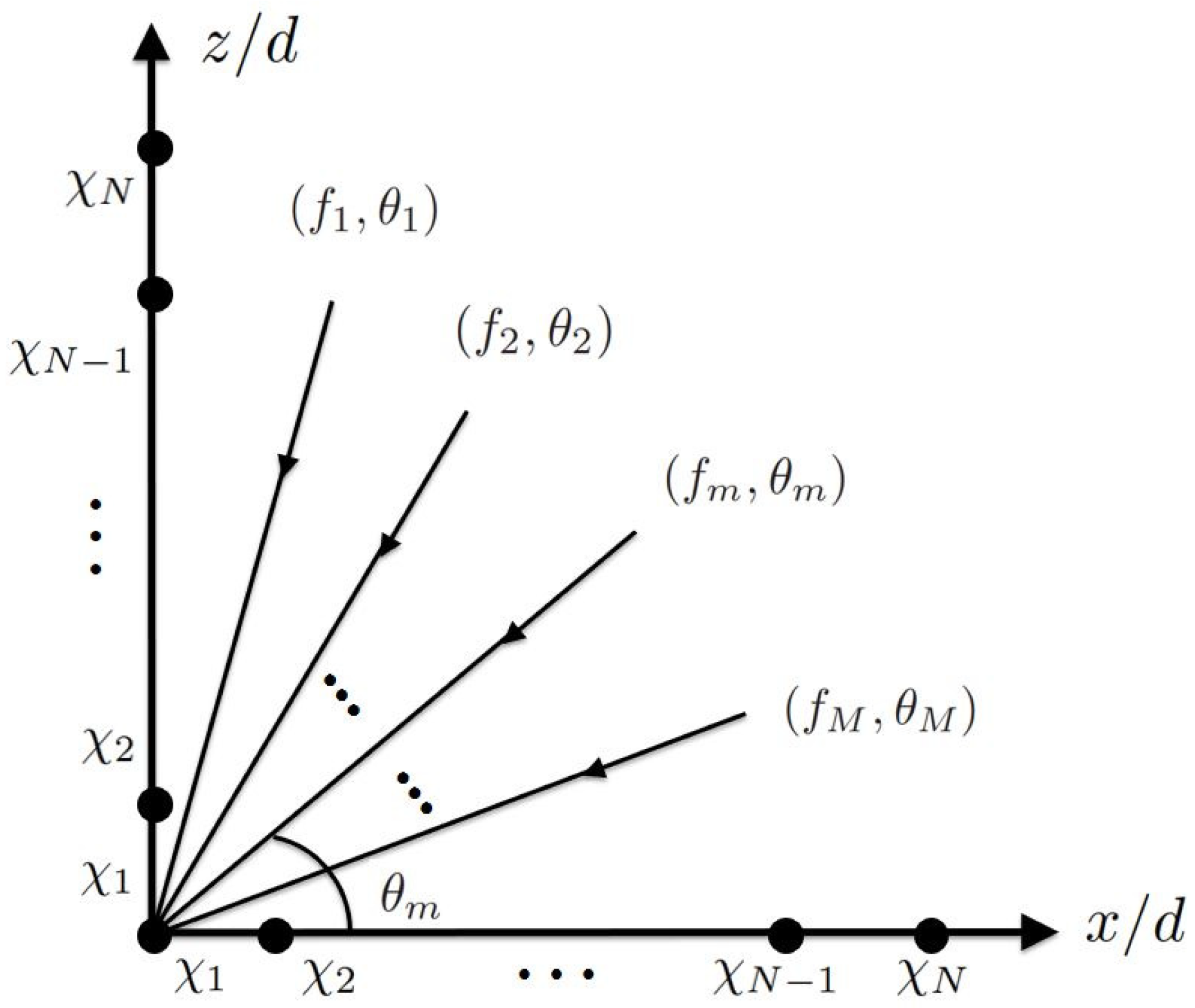
2. Signal Model
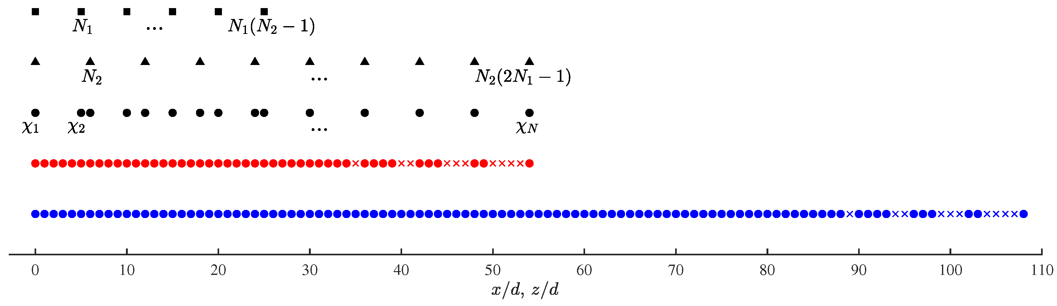
2.1. Sub-Nyquist Sampling Scheme
2.2. Second-Order Statistics
3. Joint Estimation of DOA and CF
3.1. DOA Estimation of Signal Sources with Known CF
| Algorithm 1 SS-MUSIC based on two orthogonal CPAs |
Input:
|
3.2. Joint-ESPRIT in Projected Subspace
| Algorithm 2 Projected Joint-ESPRIT (PJE) |
Input:
|
4. Simulations and Discussions
4.1. Simulation Setup
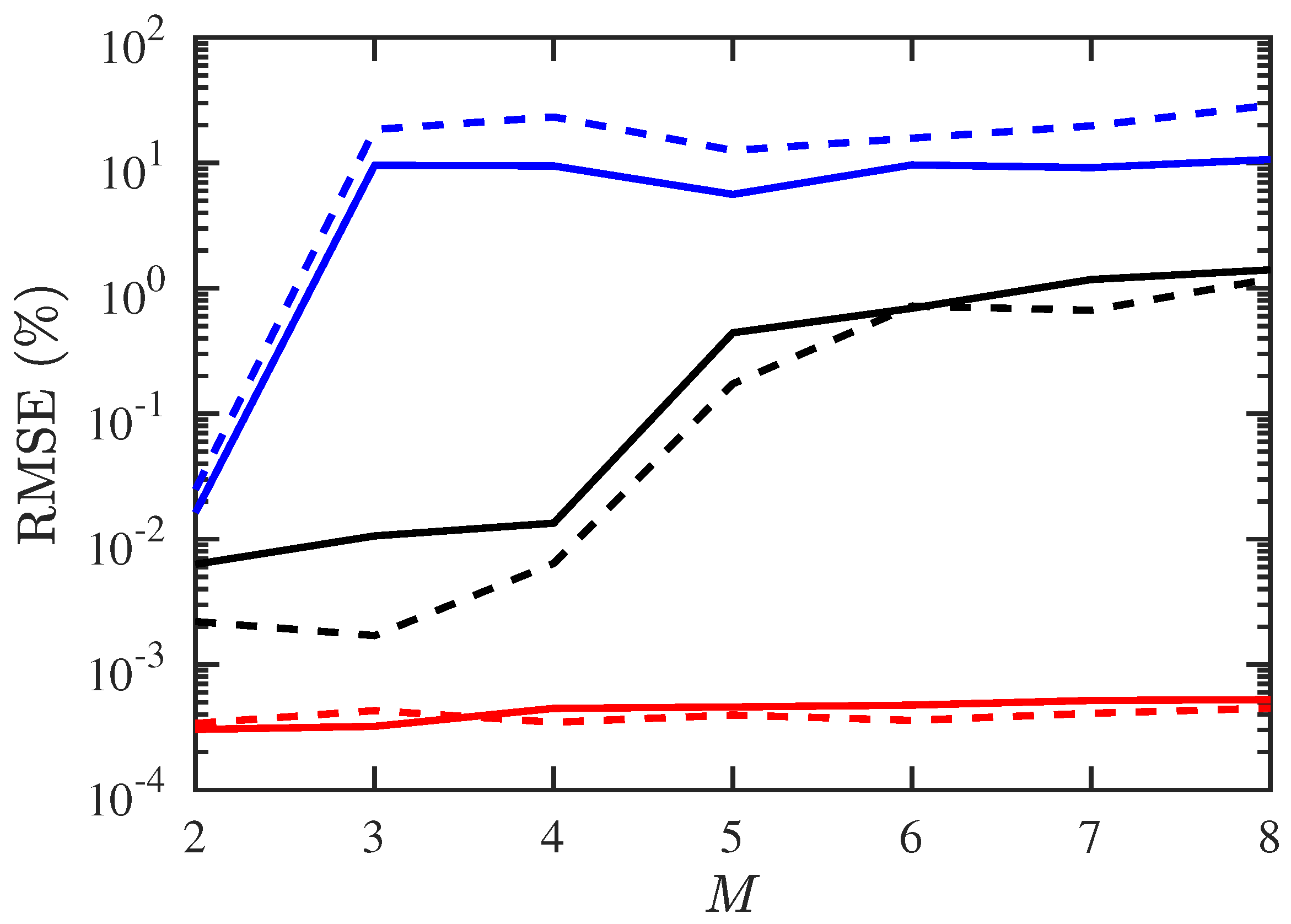
4.2. Cramer–Rao Bound
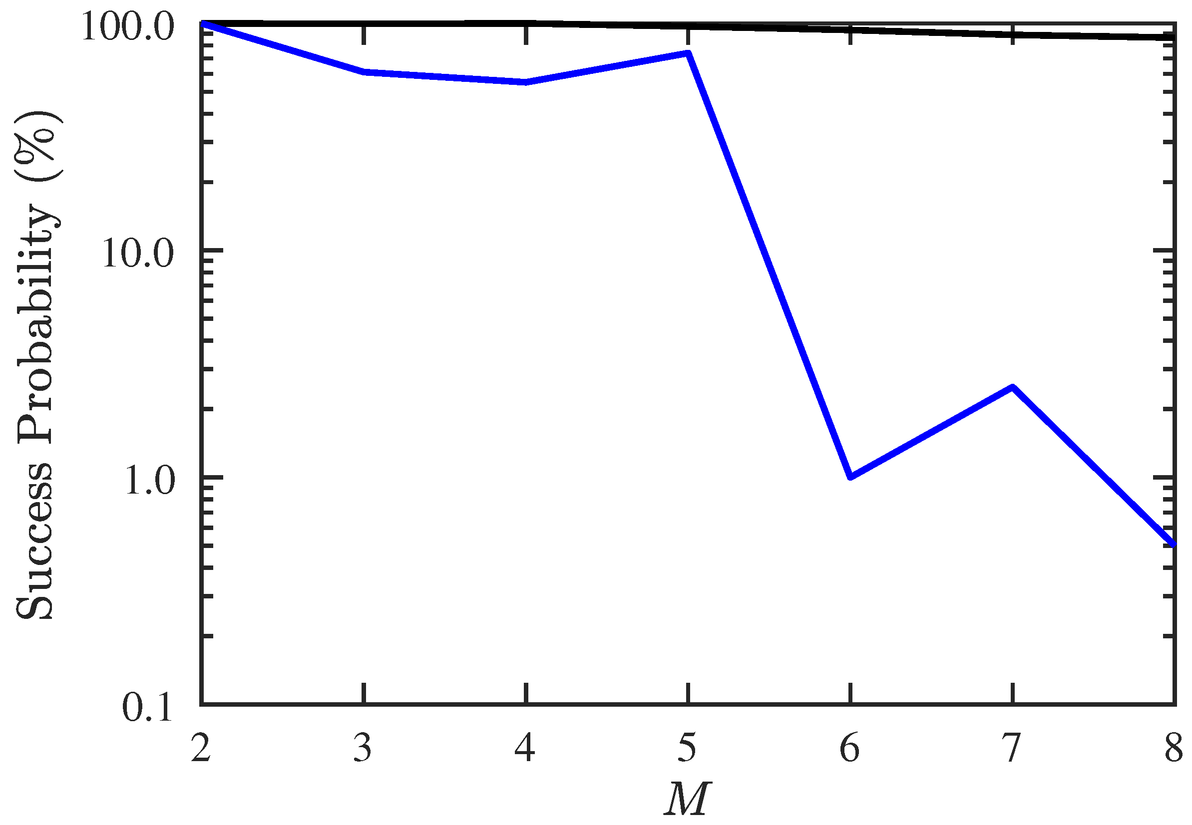
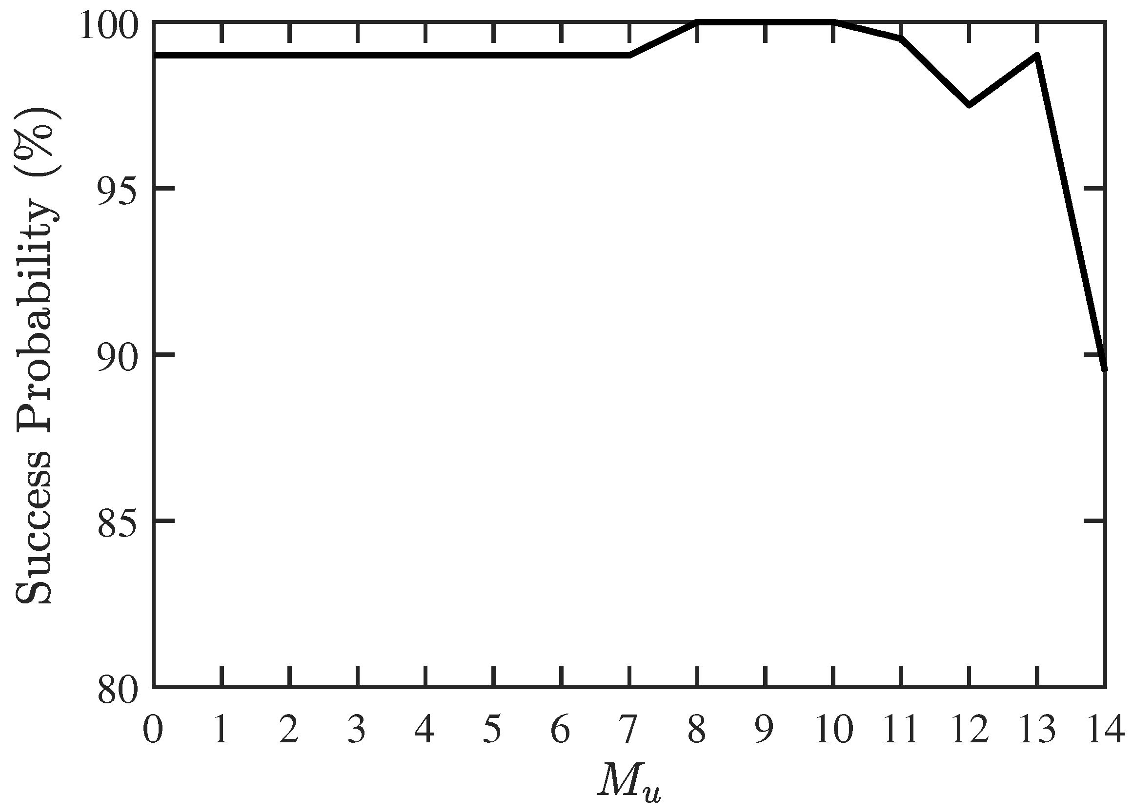
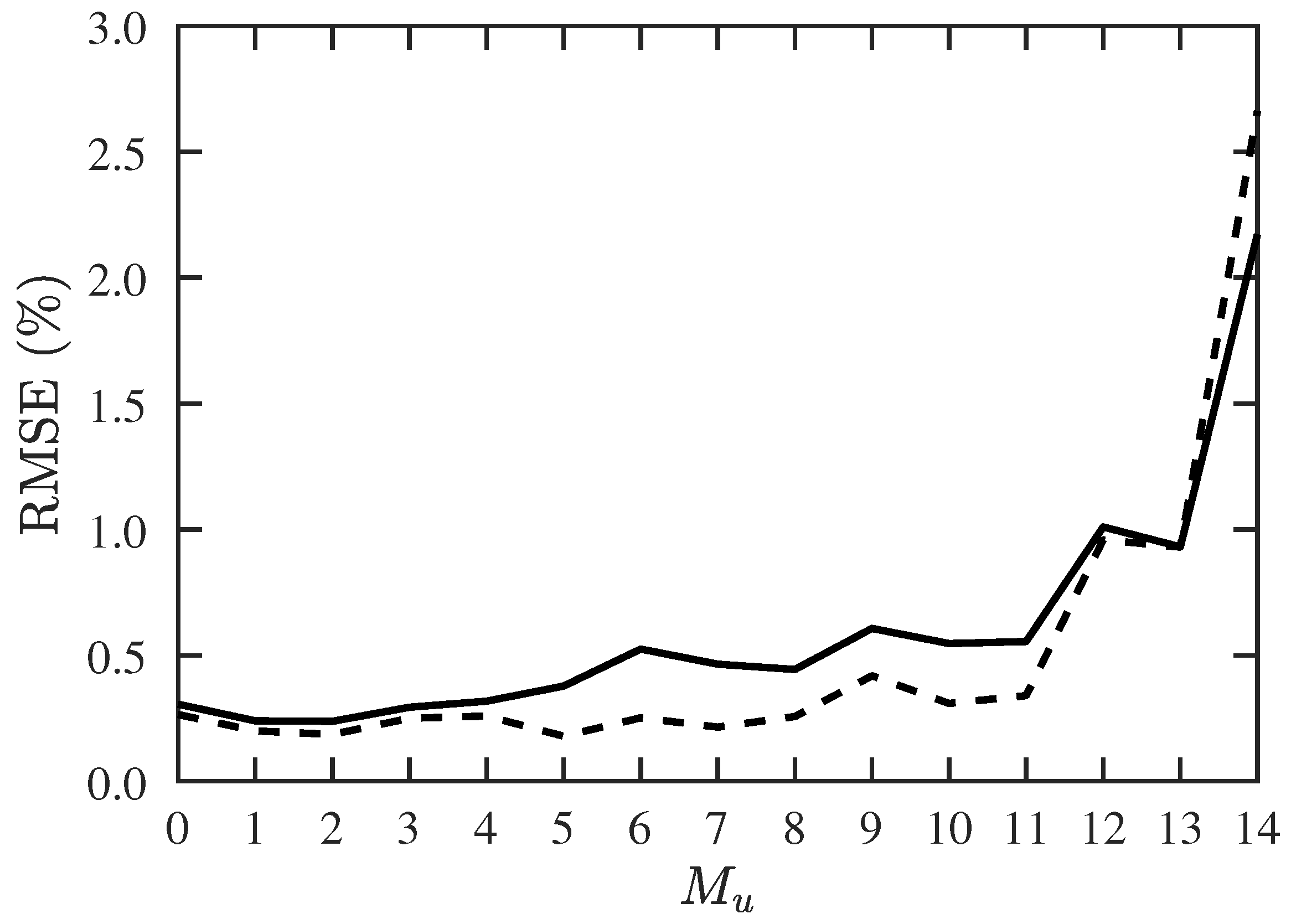
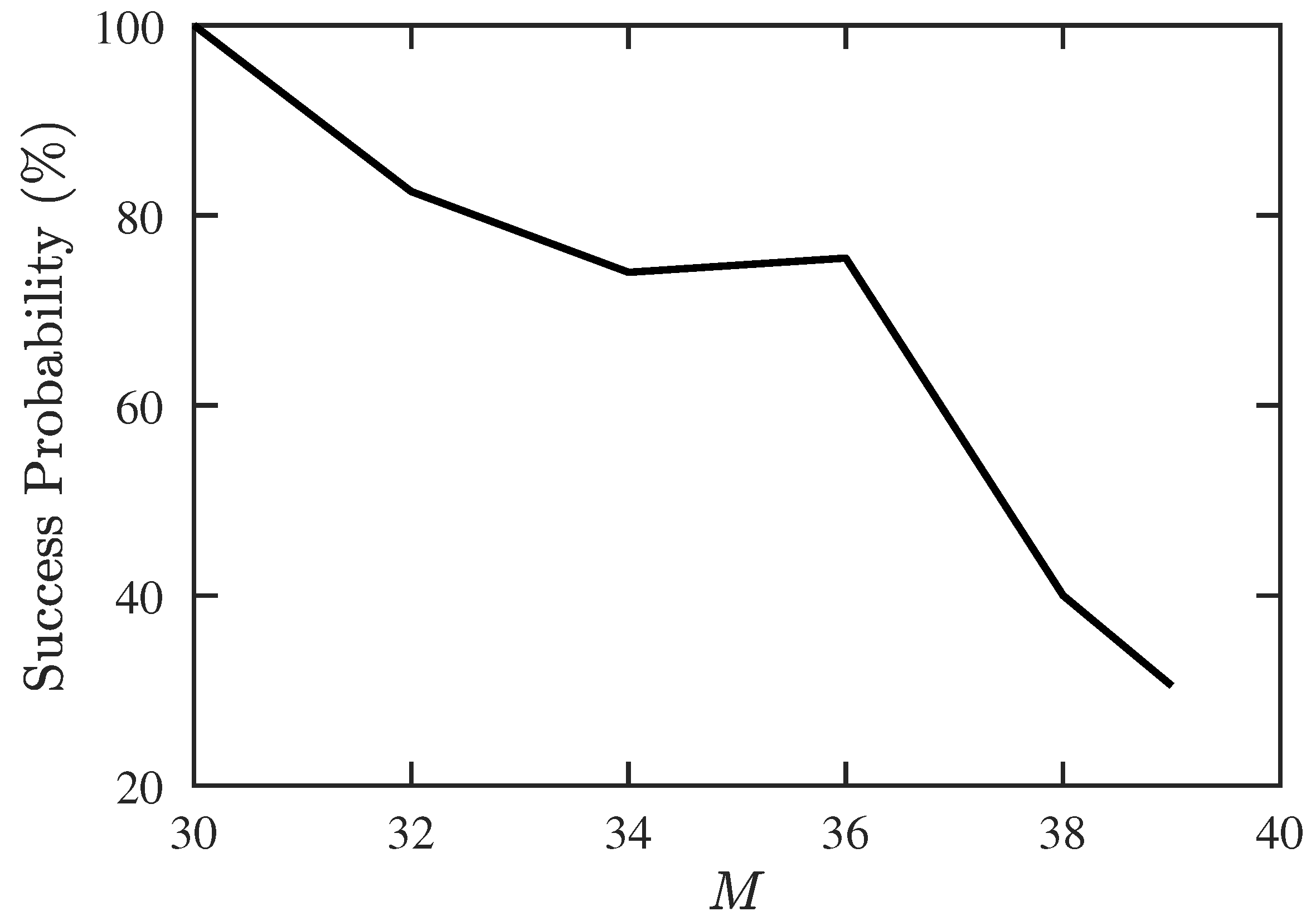
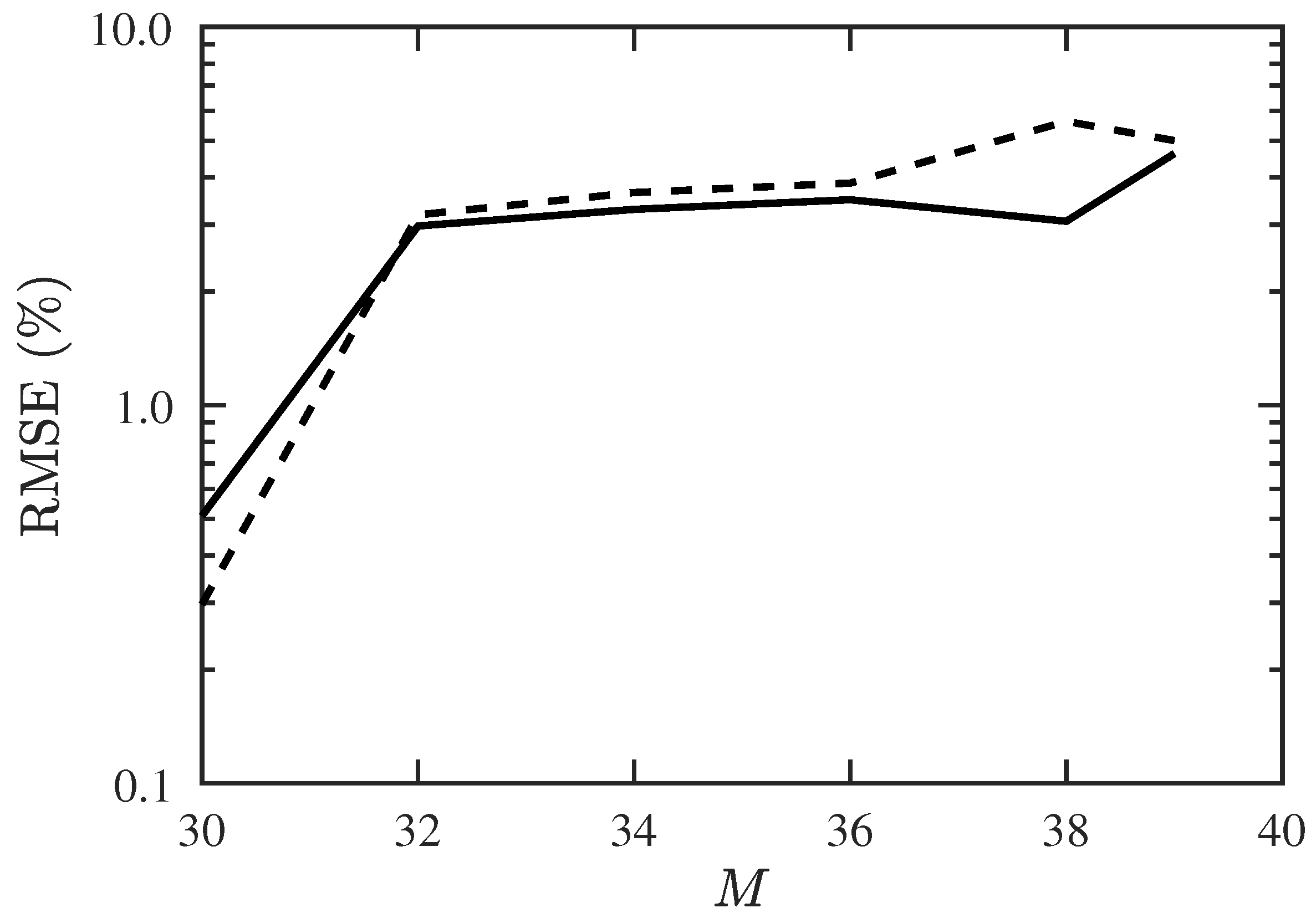
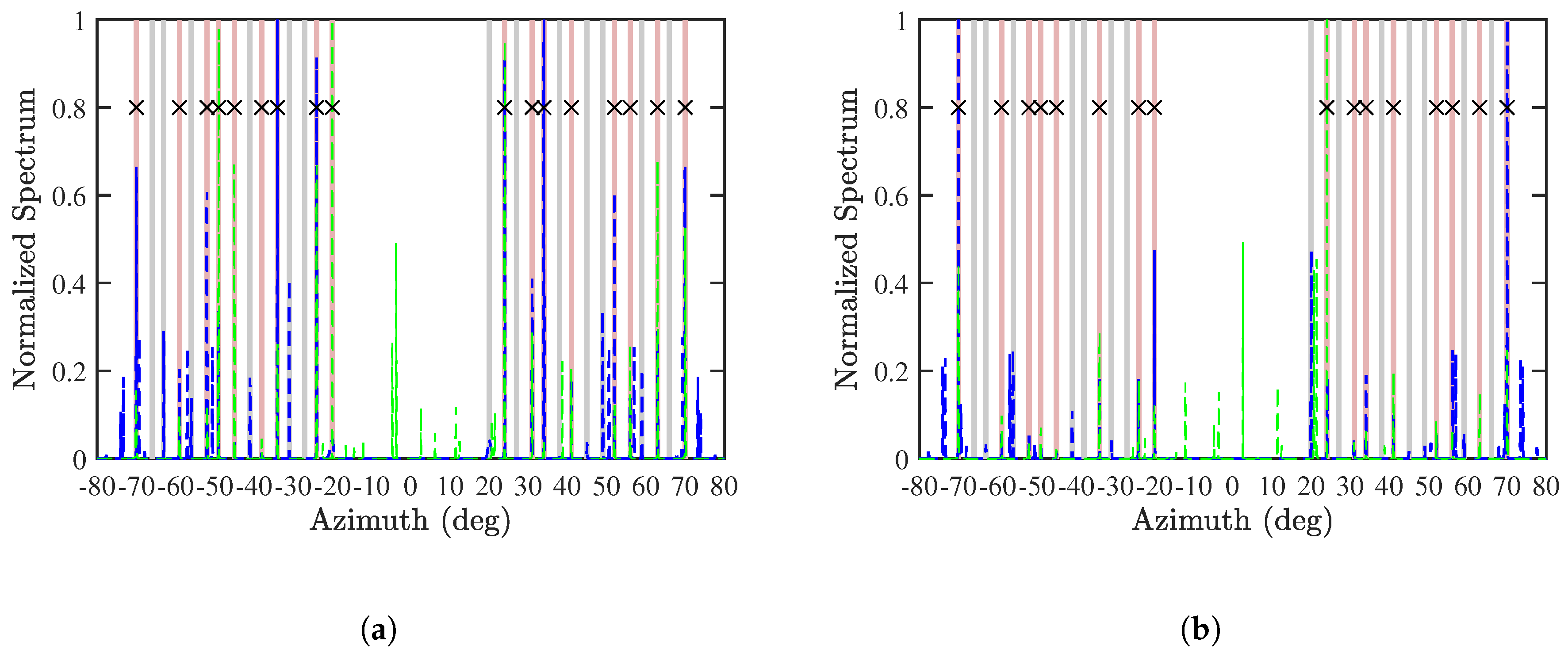
4.3. Maximum Detectable Number of Sources
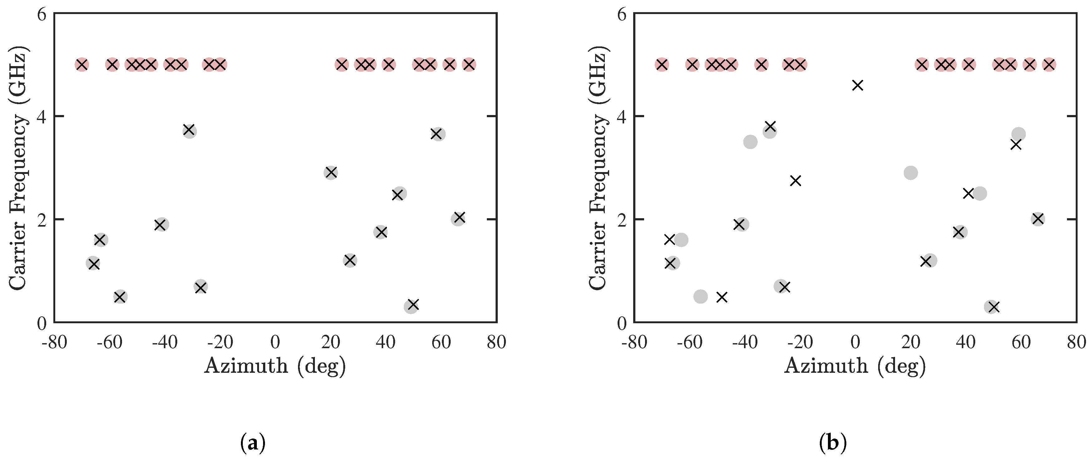
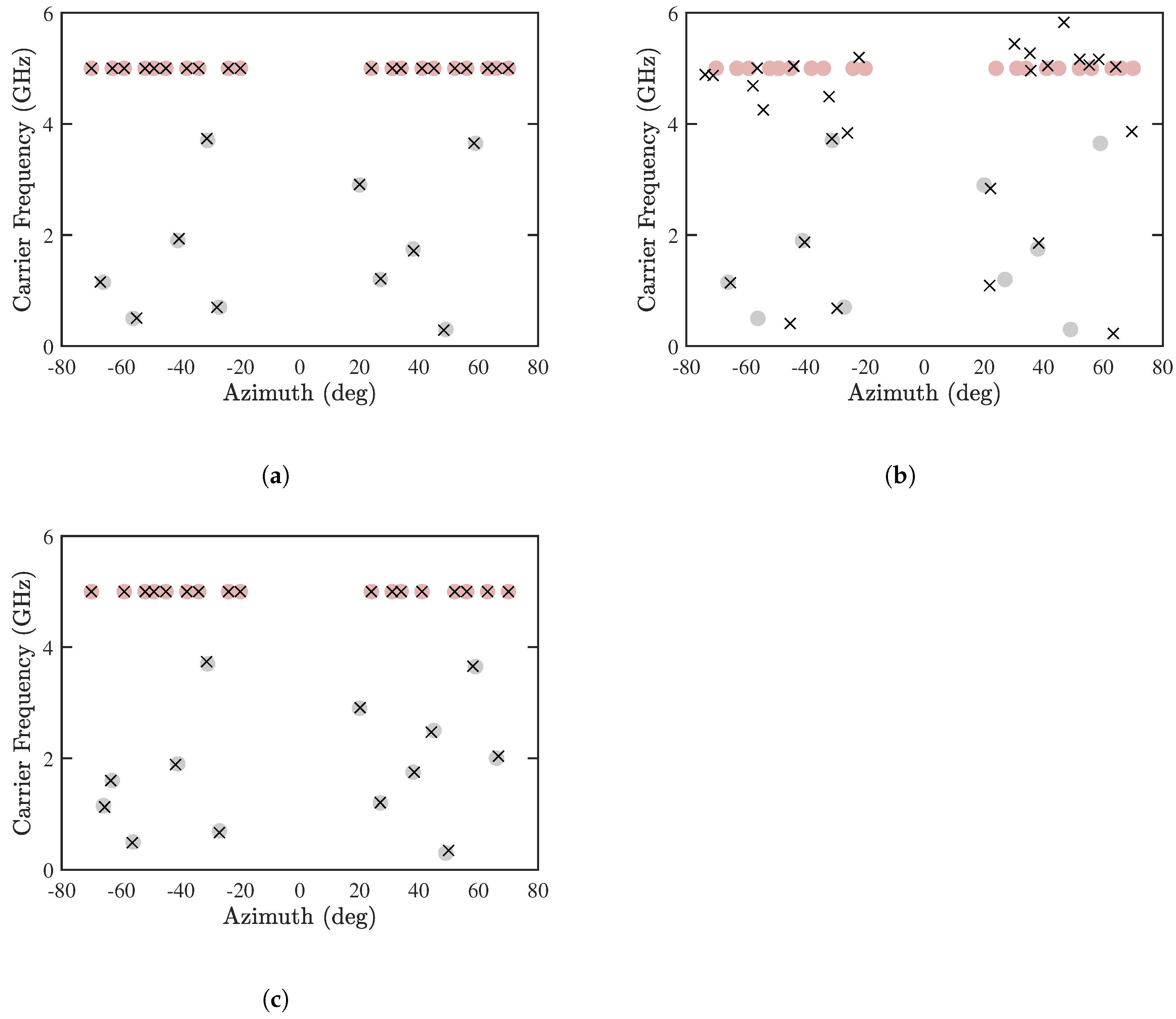
4.4. Detail of Proposed Two-Stage Algorithm
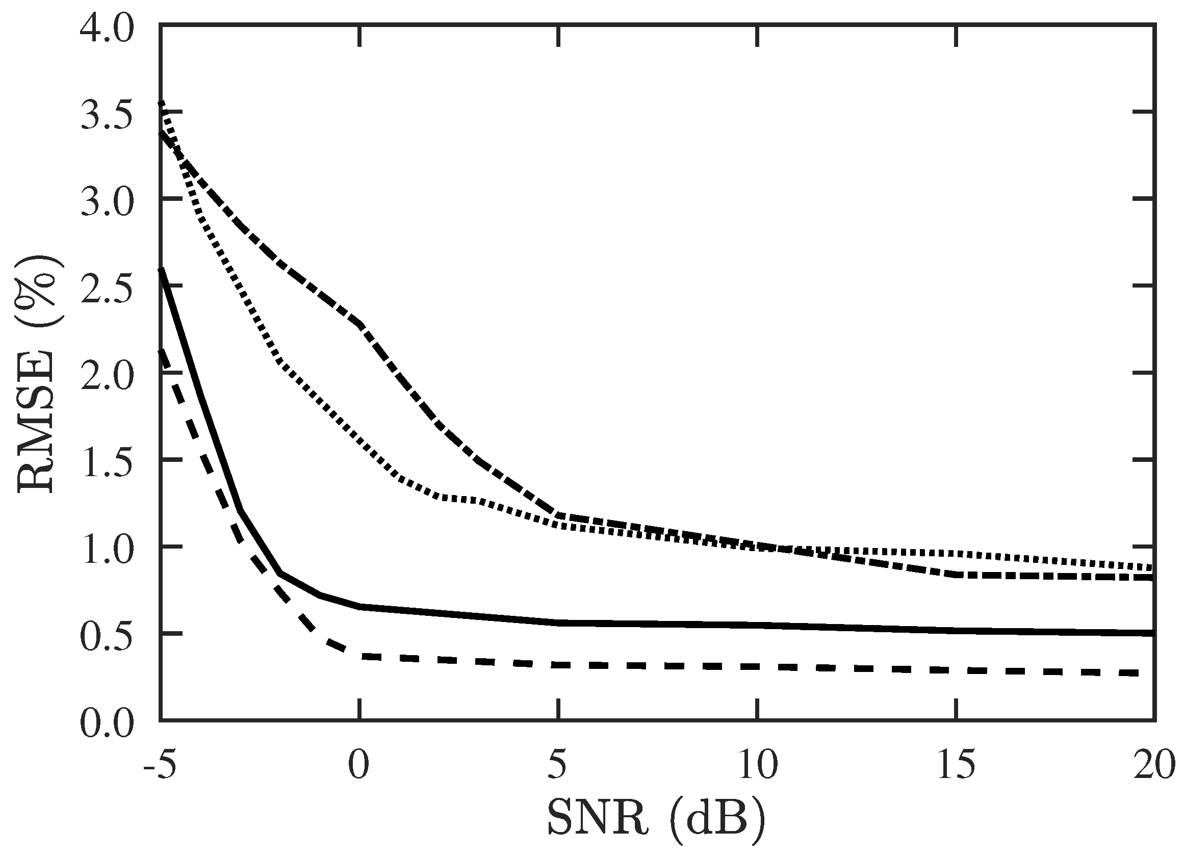
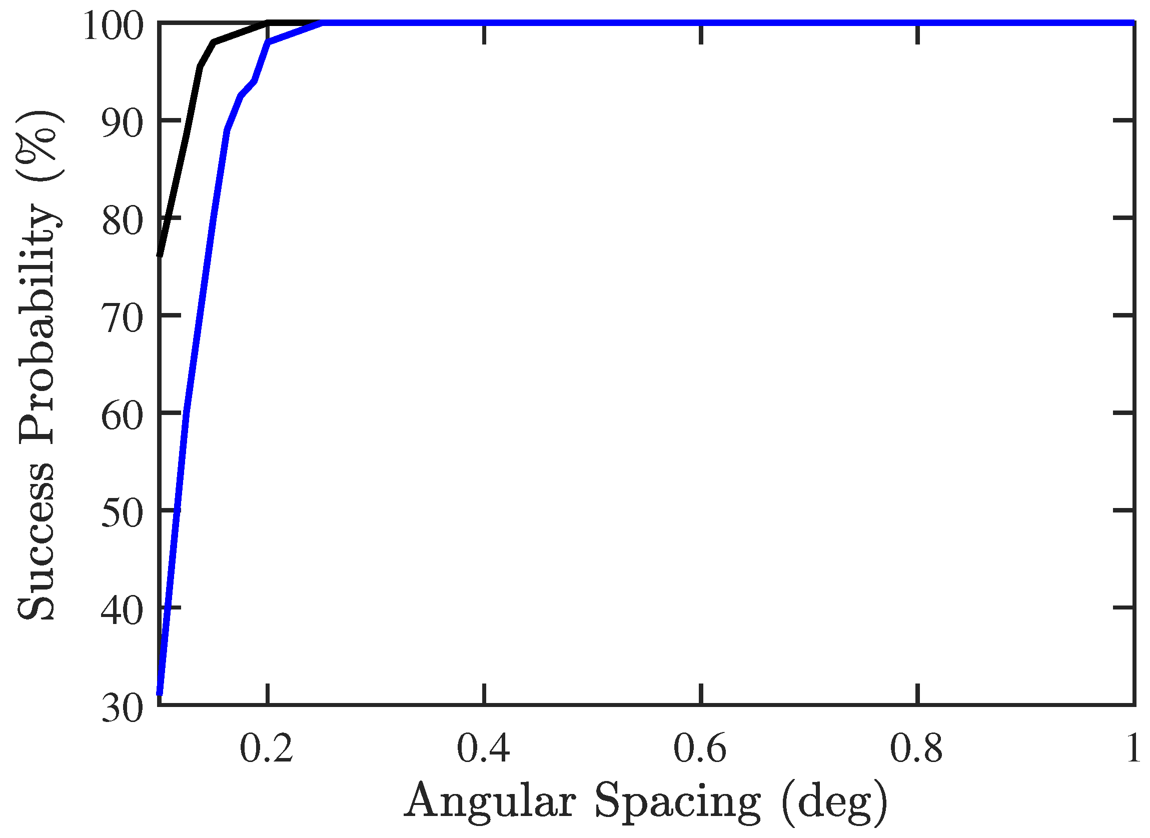
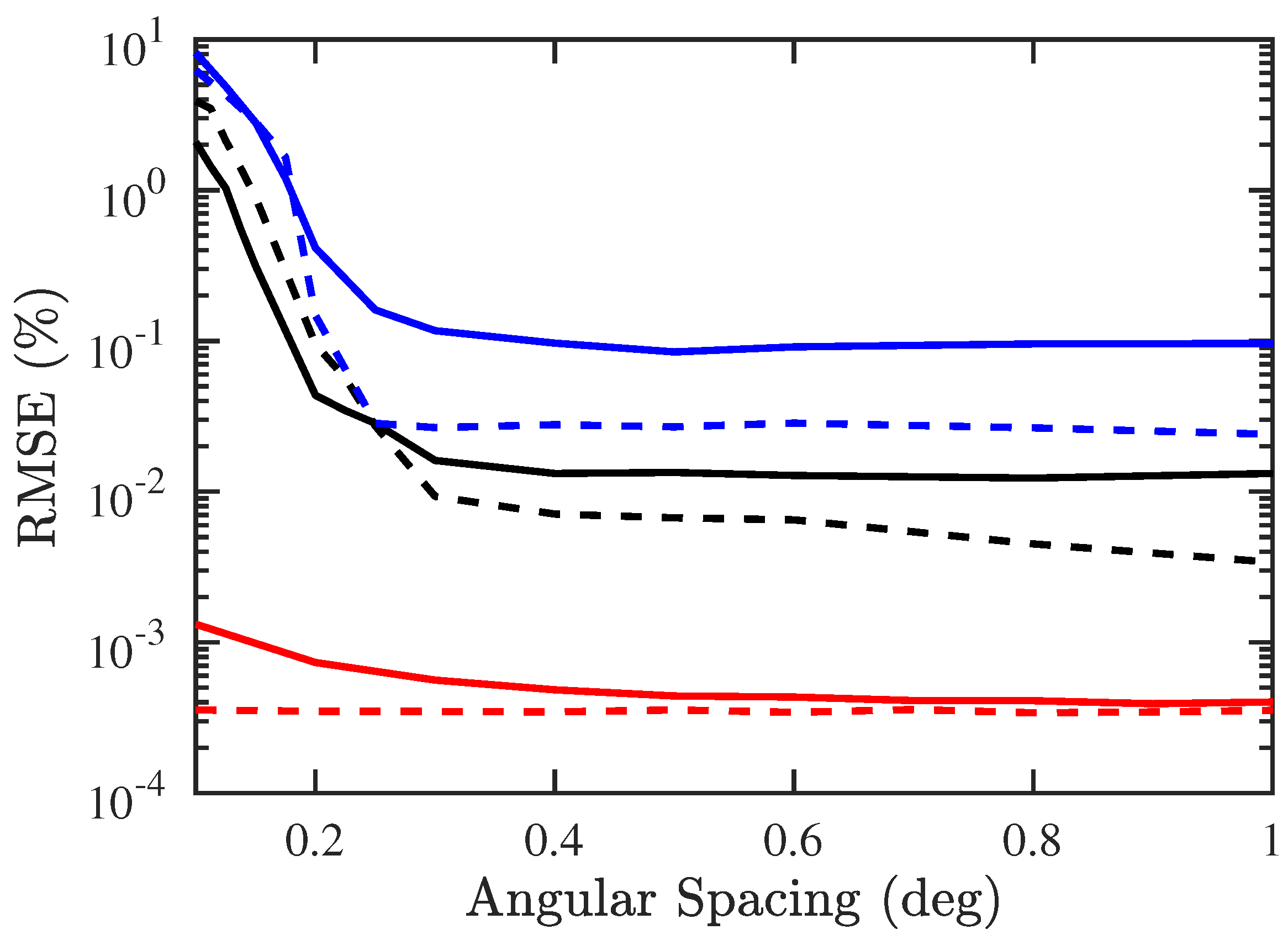
4.5. Robustness of Proposed Two-Stage Algorithm
5. Conclusions
Author Contributions
Funding
Conflicts of Interest
References
- Schmidt, R. Multiple emitter location and signal parameter estimation. IEEE Trans. Antennas Propag. 1986, 34, 276–280. [Google Scholar] [CrossRef]
- Roy, R.; Kailath, T. ESPRIT-estimation of signal parameters via rotational invariance techniques. IEEE Trans. Acoust. Speech Signal Process. 1989, 37, 984–995. [Google Scholar] [CrossRef]
- Kim, J.M.; Lee, O.K.; Ye, J.C. Compressive MUSIC: Revisiting the link between compressive sensing and array signal processing. IEEE Trans. Inf. Theory 2012, 58, 278–301. [Google Scholar] [CrossRef]
- Qin, S.; Zhang, Y.D.; Amin, M.G. Generalized coprime array configurations for direction-of-arrival estimation. IEEE Trans. Signal Process. 2015, 63, 1377–1390. [Google Scholar] [CrossRef]
- Haardt, M.; Nossek, J.A. 3-D unitary ESPRIT for joint angle and carrier estimation. IEEE Int. Conf. Acoust. Speech Signal Process. 1997, 255–258. [Google Scholar] [CrossRef]
- Dong, W.; Zhang, X.; Li, J.; Bai, J. Improved ESPRIT method for joint direction-of-arrival and frequency estimation using multiple-delay output. Int. Antennas J. Propag. 2012, 2012, 309269. [Google Scholar]
- Stein, S.; Yair, O.; Cohen, D.; Eldar, Y.C. Joint spectrum sensing and direction of arrival recovery from sub-Nyquist samples. In Proceedings of the 2015 IEEE 16th International Workshop on Signal Processing Advances in Wireless Communications (SPAWC), Stockholm, Sweden, 28 June–1 July 2015; pp. 331–335. [Google Scholar]
- Stein, S.; Yair, O.; Cohen, D.; Eldar, Y.C. CaSCADE: Compressed carrier and DOA estimation. IEEE Trans. Signal Process. 2017, 65, 2645–2658. [Google Scholar] [CrossRef]
- Lemma, A.N.; Van Der Veen, A.J.; Deprettere, E.F. Analysis of joint angle-frequency estimation using ESPRIT. IEEE J. Sel. Top. Signal Process. 2003, 51, 1264–1283. [Google Scholar] [CrossRef]
- Cui, C.; Wu, W.; Wang, W. Carrier frequency and DOA estimation of sub-Nyquist sampling multi-band sensor signals. IEEE Sens. J. 2017, 17, 7470–7478. [Google Scholar] [CrossRef]
- Mao, W.K.; Hsieh, T.H.; Chi, C.Y. DOA estimation of quasi-stationary signals with less sensors than sources and unknown spatial noise covariance: A Khatri–Rao subspace approach. IEEE Trans. Signal Process. 2010, 58, 2168–2180. [Google Scholar] [CrossRef]
- Wang, B.; Wang, W.; Gu, Y.; Lei, S. Underdetermined DOA estimation of quasi-stationary signals using a partly-calibrated array. Sensors 2017, 17, 702. [Google Scholar] [CrossRef] [PubMed]
- Hsu, K.C.; Kiang, J.F. DOA estimation of quasi-stationary signals using a partly-calibrated uniform linear array with fewer sensors than sources. Prog. Electromagn. Res. M 2018, 63, 185–193. [Google Scholar] [CrossRef]
- Pal, P.; Vaidyanathan, P.P. Nested arrays: A novel approach to array processing with enhanced degrees of freedom. IEEE Trans. Signal Process. 2010, 58, 4167–4181. [Google Scholar] [CrossRef]
- Vaidyanathan, P.P.; Pal, P. Sparse sensing with co-prime samplers and arrays. IEEE Trans. Signal Process. 2011, 59, 573–586. [Google Scholar] [CrossRef]
- Pal, P.; Vaidyanathan, P.P. Coprime sampling and the MUSIC algorithm. In Proceedings of the 2011 Digital Signal Processing and Signal Processing Education Meeting (DSP/SPE), Sedona, AZ, USA, 4–7 January 2011; pp. 289–294. [Google Scholar]
- Shen, Q.; Liu, W.; Cui, W.; Wu, S. Extension of co-prime arrays based on the fourth-order difference co-array concept. IEEE Signal Process. Lett. 2016, 23, 615–619. [Google Scholar] [CrossRef]
- Hsu, K.C.; Kiang, J.F. DOA estimation using triply primed arrays based on fourth-order statistics. Prog. Electromagn. Res. M 2018, 67, 55–64. [Google Scholar] [CrossRef]
- Chen, K.H.; Kiang, J.F. Coupling characterization of a linear dipole array to improve direction-of-arrival estimation. IEEE Trans. Antennas Propag. 2015, 63, 5056–5062. [Google Scholar] [CrossRef]
- Adve, R.S.; Sarkar, T.K. Compensation for the effects of mutual coupling on direct data domain adaptive algorithms. IEEE Trans. Antennas Propag. 2000, 48, 86–94. [Google Scholar] [CrossRef]
- Dandekar, K.R.; Ling, H.; Xu, G. Experimental study of mutual coupling compensation in smart antenna applications. IEEE Trans. Wirel. Commun. 2002, 1, 480–487. [Google Scholar] [CrossRef]
- Morales-Jimenez, D.; Raymond Louie, H.Y.; McKay, M.R.; Chen, Y. Analysis and design of multiple-antenna cognitive radios with multiple primary user signals. IEEE Trans. Signal Process. 2015, 63, 4925–4939. [Google Scholar] [CrossRef]
- Liu, C.L.; Vaidyanathan, P. Remarks on the spatial smoothing step in coarray MUSIC. IEEE Signal Process. Lett. 2015, 22, 1438–1442. [Google Scholar] [CrossRef]
- Stoica, P.; Nehorai, A. MUSIC, maximum likelihood, and Cramer–Rao bound. IEEE Trans. Acoust. Speech Signal Process. 1989, 37, 720–741. [Google Scholar] [CrossRef]
- Stoica, P.; Nehorai, A. Performance study of conditional and unconditional direction-of-arrival estimation. IEEE Trans. Acoust. Speech Signal Process. 1990, 38, 1783–1795. [Google Scholar] [CrossRef]
- Chen, H.; Hou, P.; Wang, Q.; Huang, L.; Yan, W.-Q. Cumulants-based Toeplitz matrices reconstruction method for 2-D coherent DOA estimation. IEEE Sens. J. 2014, 14, 2824–2832. [Google Scholar] [CrossRef]
- Wang, X.; Mao, X.; Wang, Y.; Zhang, N.; Li, B. A novel 2-D coherent DOA estimation method based on dimension reduction sparse reconstruction for orthogonal arrays. Sensors 2016, 16, 1496. [Google Scholar] [CrossRef] [PubMed]


© 2019 by the authors. Licensee MDPI, Basel, Switzerland. This article is an open access article distributed under the terms and conditions of the Creative Commons Attribution (CC BY) license (http://creativecommons.org/licenses/by/4.0/).
Share and Cite
Hsu, K.-C.; Kiang, J.-F. Joint Estimation of DOA and Frequency of Multiple Sources with Orthogonal Coprime Arrays. Sensors 2019, 19, 335. https://doi.org/10.3390/s19020335
Hsu K-C, Kiang J-F. Joint Estimation of DOA and Frequency of Multiple Sources with Orthogonal Coprime Arrays. Sensors. 2019; 19(2):335. https://doi.org/10.3390/s19020335
Chicago/Turabian StyleHsu, Kai-Chieh, and Jean-Fu Kiang. 2019. "Joint Estimation of DOA and Frequency of Multiple Sources with Orthogonal Coprime Arrays" Sensors 19, no. 2: 335. https://doi.org/10.3390/s19020335
APA StyleHsu, K.-C., & Kiang, J.-F. (2019). Joint Estimation of DOA and Frequency of Multiple Sources with Orthogonal Coprime Arrays. Sensors, 19(2), 335. https://doi.org/10.3390/s19020335