Abstract
Knowledge-based NMR spectral prediction relies on the correlations between substructures and sub-spectra. To extract the correlations, a systematic substructure measurement has been developed to classify substructures according to their chemical shift values. Historically, the atom center fragment (ACF) concept has been used as a means to systematically measure substructures for NMR spectral prediction. The assumption behind this concept is that the chemical shift value of an atom is influenced by its chemical environment. Based upon the study of the ACF-type approaches, a generalized atom center fragment (GACF) approach is proposed in this paper. In the GACF approach, a substructure consists of a center atom, core layer, and external layers. The center atom and the core layer, are identified as the super center atom. The external layers are the chemical environment. A number of algorithms have been developed to measure GACF substructures from a structure database, and create the NMR knowledge base for NMR spectral prediction.
Introduction
Empirical NMR spectral prediction approaches correlate substructures and sub-spectra by means of sub-structural encoding. The oldest encoding method is the additivity model, which consists of a set of frame structures, substituents, and calculation rules [1,2]. A more general additivity model was reported by the Small and Jurs [3], and enhanced by Schweitzer and Small [4] later. Recently, a number of neural network approaches have been employed for the encoding [5,6,7,8]. Bremser proposed HOSE code to systematically encode substructures for 13C NMR knowledge extraction [9]. Robien adopted HOSE method [10], and built up a direct knowledge base retrieval method for 13C NMR spectral prediction [11]. His newer publications can be found from Anal. Chim. Acta , 1990, 229, 17 and J. Chem. Inf. Comput. Sci., 1992, 32, 291.
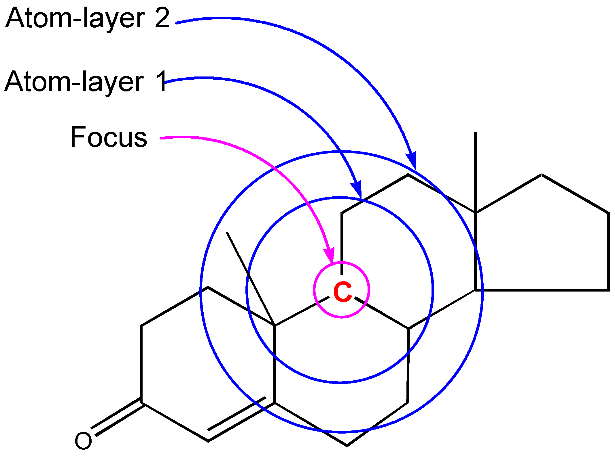
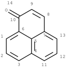
The critical part of NMR knowledge generation is the systematic substructure measurement. The chemical shift value of a carbon atom is influenced by the chemical environment of the atom. HOSE code uses layer (or level) to define the chemical environment (Figure 1). The first layer is defined as all the atoms being one-bond-away from the central atom (or focus atom); the second layer has the atoms being two-bond-away, etc. This idea can be represented in atom center fragment (ACF) concept, which has been addressed by many authors in different ways [12,13,14].
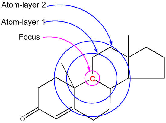
Figure 1.
The center atom (focus atom) and atom layers in HOSE code approach.
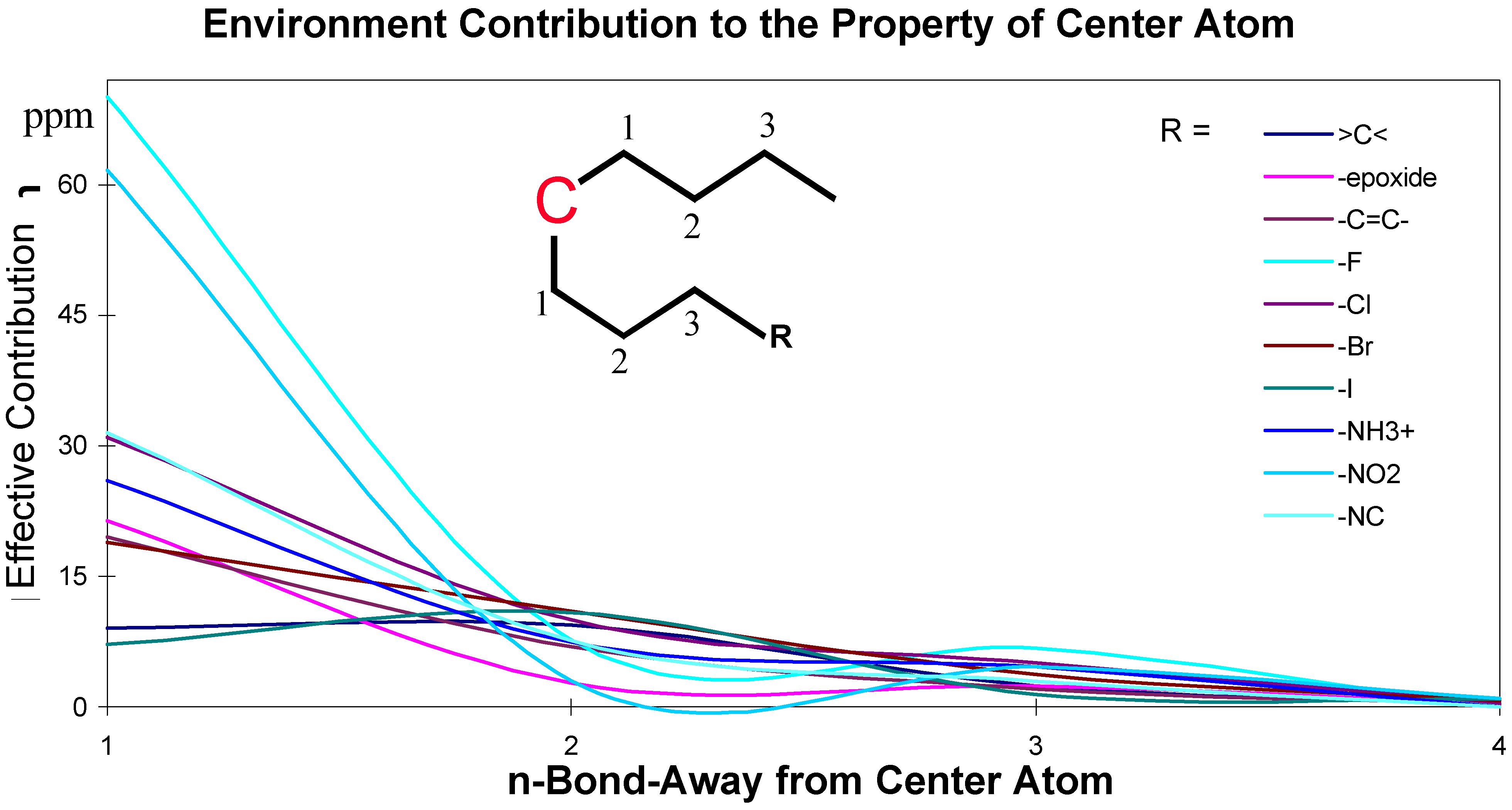
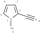
The effects of the environmental atoms on the central atom are not completely determined by the topological distance between the center atom and the environmental atoms. The effects are influenced by the topological distance and the bonding types. These effective contributions of environmental atoms/groups to the central atom are shown in Figure 2 and Figure 3.
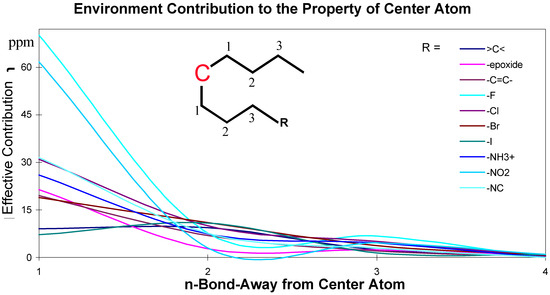
Figure 2.
Chemical environment effective contribution to a central carbon atom in an aliphatic structure.
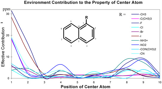
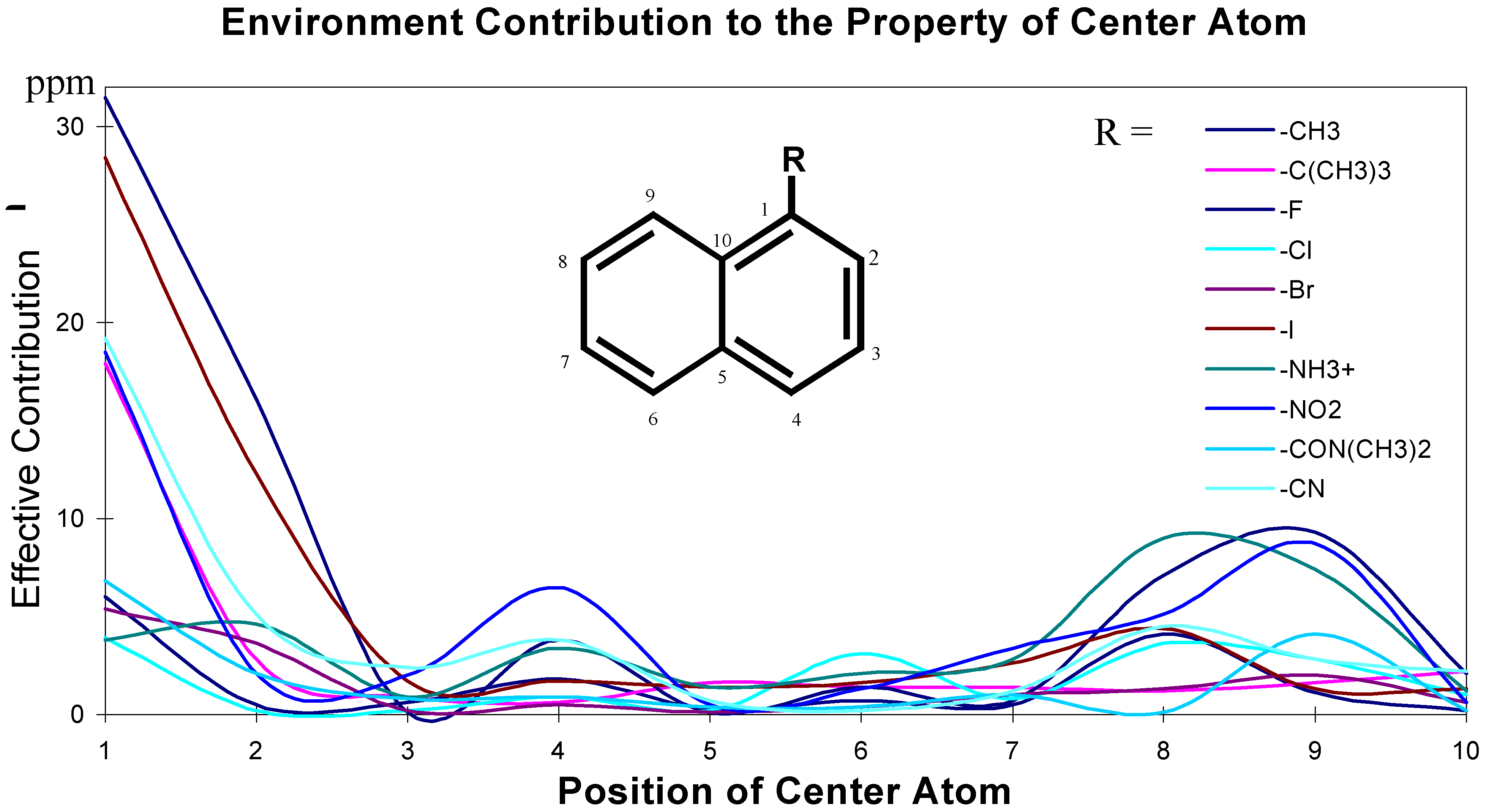
Figure 3.
Chemical environment and its effect on central carbon atoms in aromatic system.
The data for these Figures are adopted from reference 1; the plots use the chemical shift absolute values to emphasize the contributions. Figure 2 and Figure 3 are just showing the tendency, the continuous curves do not mean there is any effective contribution between 1-bond-away and 2-bond-away, etc.
From these Figures, it can be seen that if a center atom is in an acyclic aliphatic system, the effect of an environmental substituent to the center atom decreases along the increasing number of the atom-layer. If the substituent is four bonds away from the center atom, it has almost no effective contribution to change the center atom’s chemical shift. In Figure 3, however, even R-group is at the position 4 (four-bonds-away), its effect on the center atom’s chemical shifts is still significant. It is because the center atom is in an aromatic system.
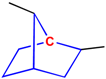
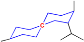
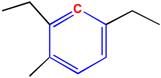
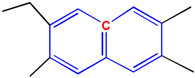
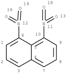
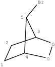
The conclusion from these Figures is that the simple ACF measurement works only for acyclic and non-conjugated systems. Another problem in the simple ACF approach is that the number of atom layers should be included in an ACF substructure. For example, if an ACF includes four atom layers, then it may be too far for the center atom in an aliphatic system, but not far enough for the one in a ring or conjugated system (see Figure 4).
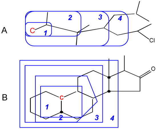
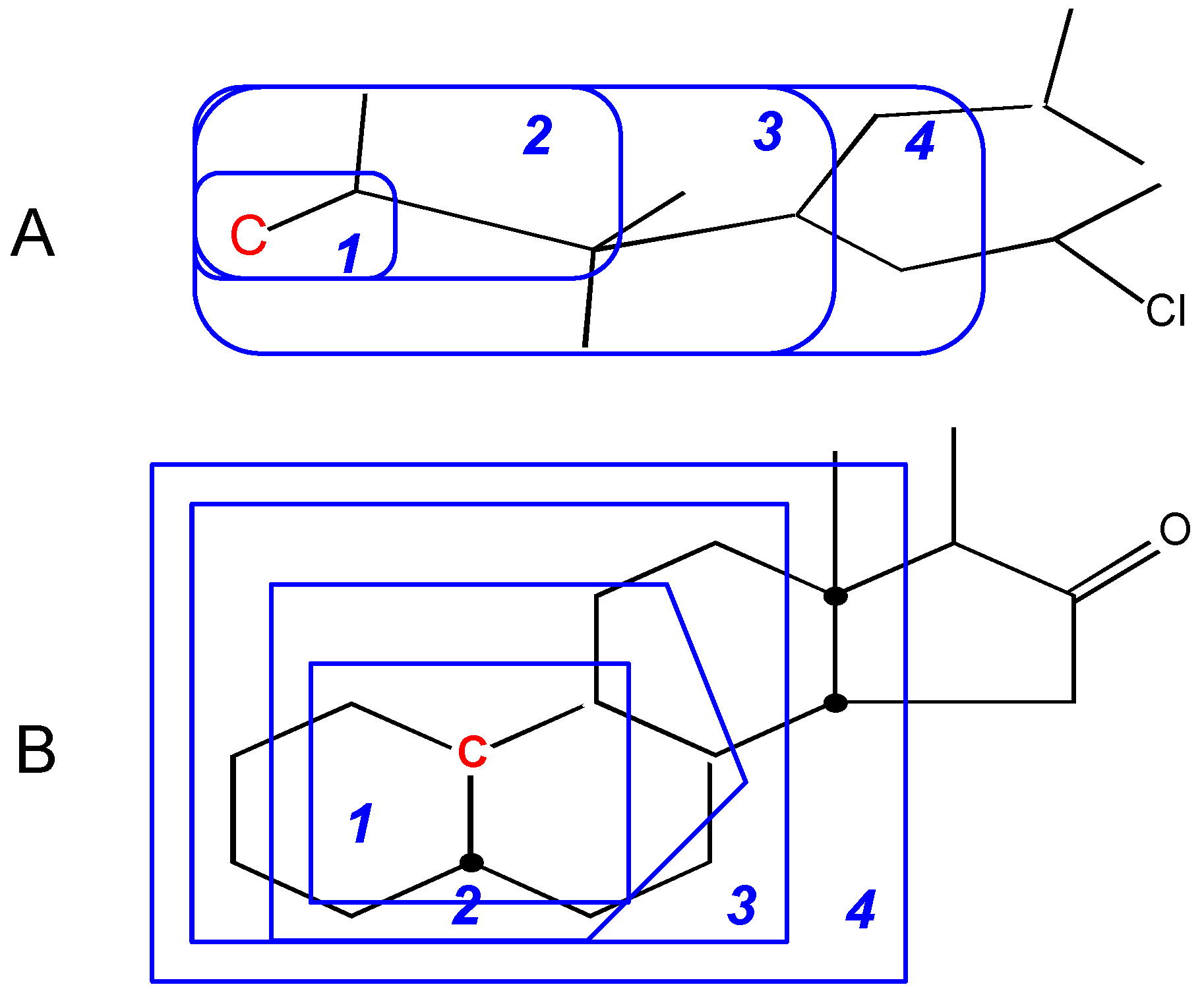
Figure 4.
Atom layers in different systems. A: Layer 4 is too far for this center atom (in red color). B: Layer 4 is still not far enough for this center atom (in red color). The numbers represent atom layers.
To have an objective substructure measurement, it is necessary to extend the simple ACF concept to generalized atom center fragment concept.
Generalized atom center fragment (GACF)
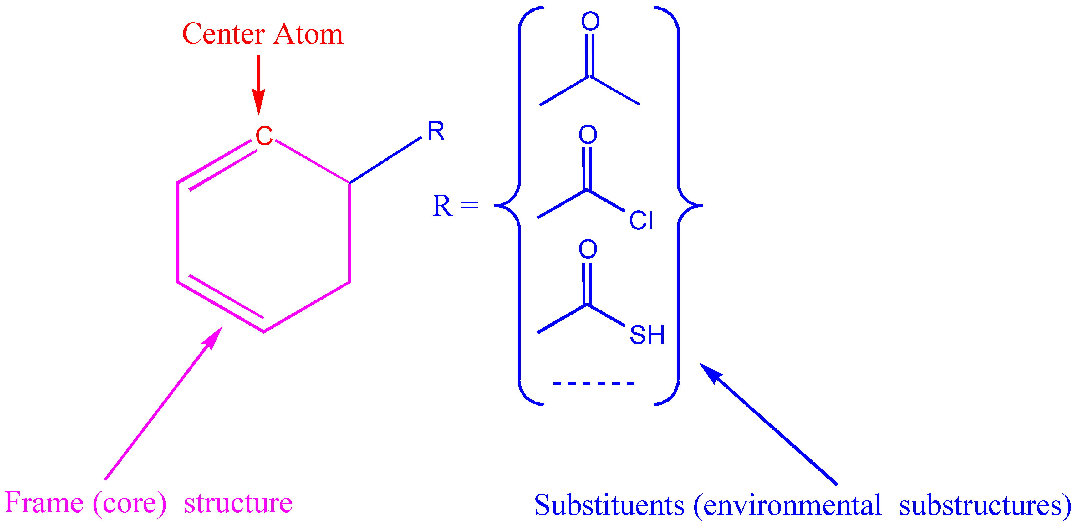
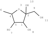
In the additivity model, the chemical environment of a center atom has two parts (see Figure 5), i.e., frame (core) structure and substituents (environmental substructures).
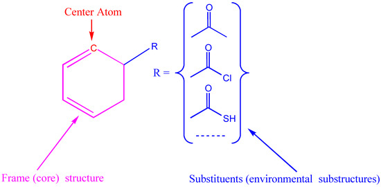
Figure 5.
Center atom, core structure and environmental substructures.
The GACF approach takes this into account in the substructure measurement. A GACF substructure consists of a center atom, core structure and environmental layers (substituents). The core structure characterizes the different bonding system, which is also responsible for the special chemical behavior. According to topological and chemical properties, core structures are classified into the following nine classes:
- Independent non-aromatic single ring system
- Fused non-aromatic ring system
- Bridged ring system
- Spiro ring system
- Independent aromatic single ring system
- Fused aromatic ring system
- Conjugated system
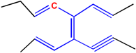
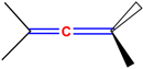
- Cumulene system
- Acyclic system
The structural features of these systems are listed in Table 1.

Table 1.
Core structure classification*
A core structure can be classified into more than one ring class simultaneously. In this case, the assigned class is chosen by applying priority:
spiro ring > bridged ring > fused ring
The examples are shown in Figure 6.
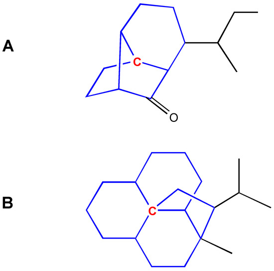
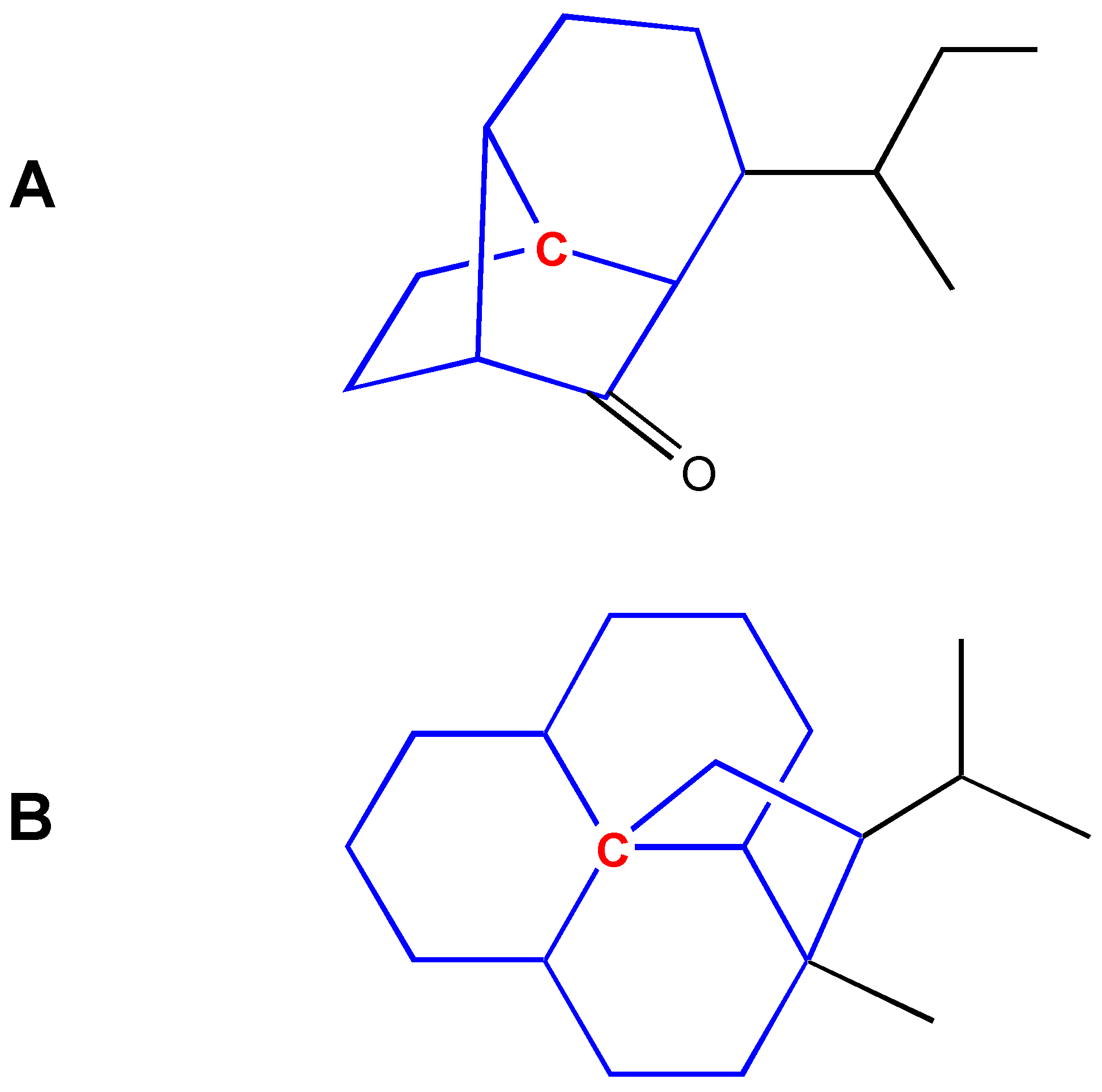
Figure 6.
Choosing a ring class for an ambiguous center atom. A: the center atom is in bridged ring and fused ring systems; it is assigned to bridged ring system. B: the center atom is in fused ring, bridged ring and spiro ring systems; it is assigned to spiro ring system.
Therefore, a GACF substructure is measured in the following steps:
- select a center atom
- get a class for the center atom
- capture a core structure for the center atom (the core structure measurement is shown in blue in Table 1 in the right column)
- capture environmental substituents (which are part of the GACF) for the GACF according to the number of the layers
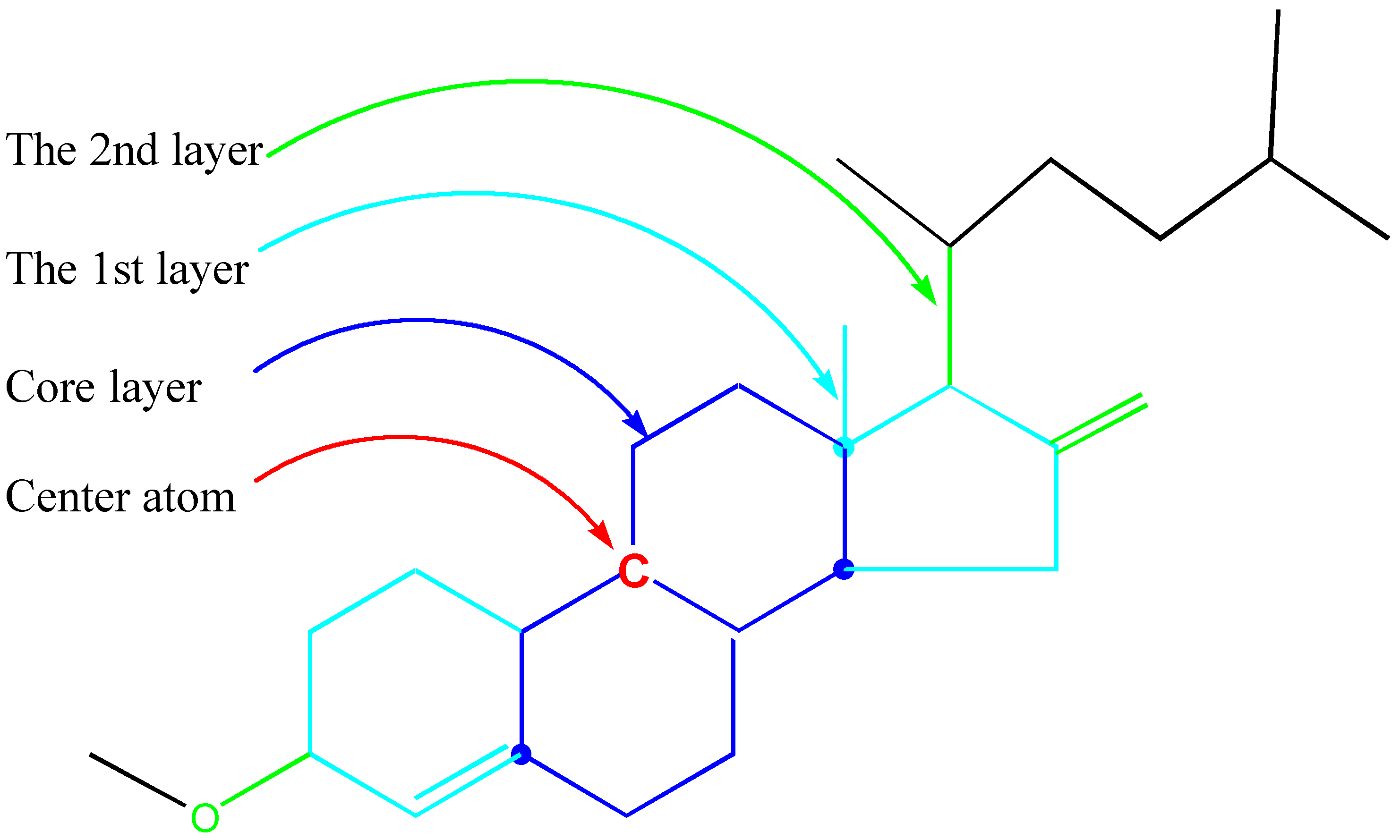
An GACF example is illustrated in Figure 7.
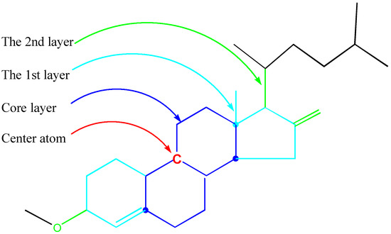
Figure 7.
Example of a GACF.
13C NMR knowledge extraction and chemical shift prediction
50,000 structures with 13C chemical shift assignments have been selected as input data set for 13C NMR knowledge extraction. A number of graph theory algorithms have been developed to measure GACF substructures. The main algorithms are independent ring, fused ring, bridged ring, spiro ring perception algorithms, and conjugated system perception algorithm, etc. These algorithms are all based upon the GMA algorithm reported in our previous work [15].
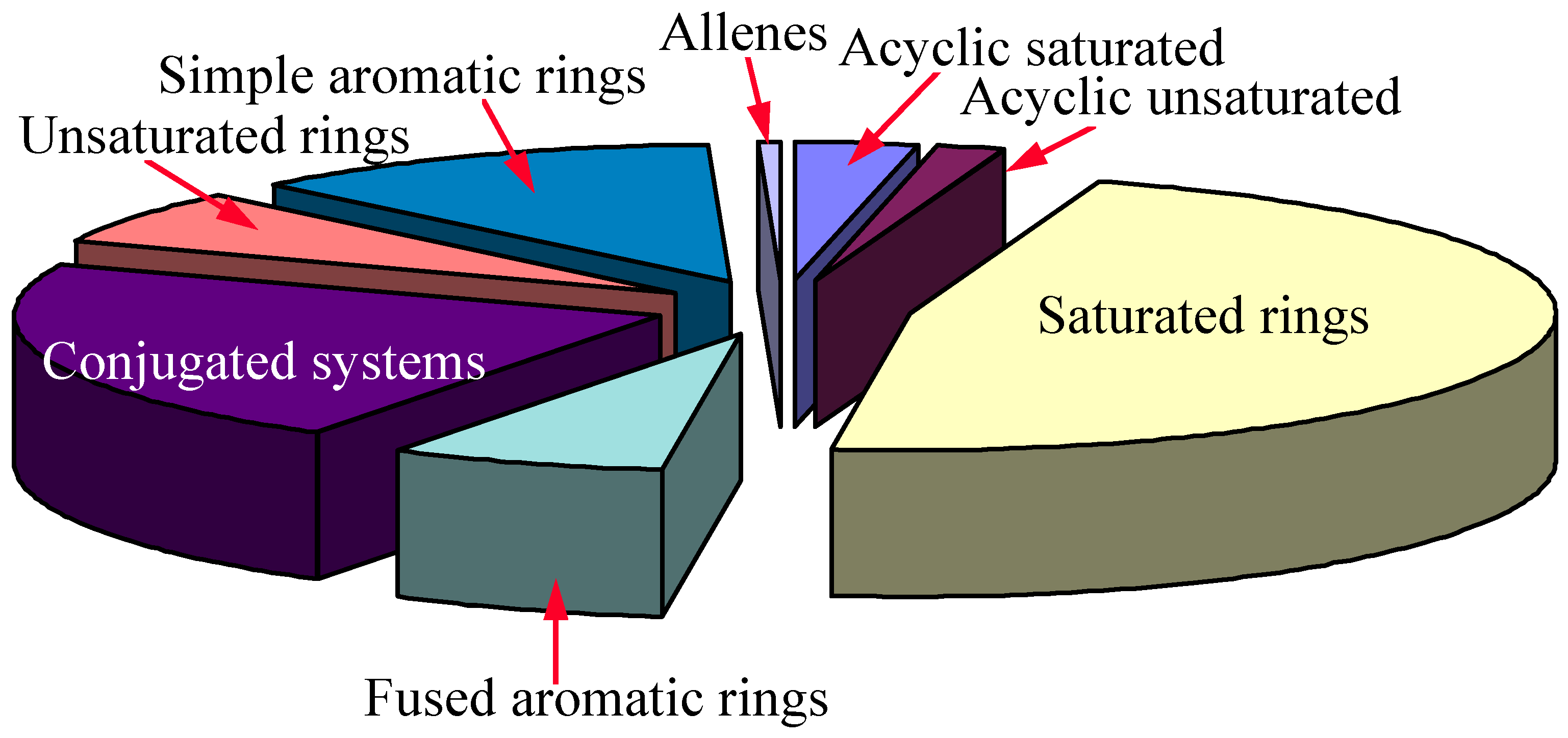
The molecular diversity of the input data has been analyzed by means of our in-house algorithms, and shown in Figure 8.
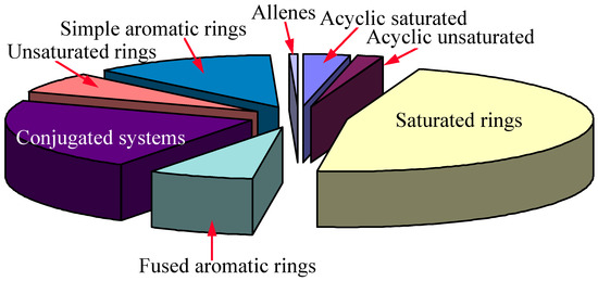
Figure 8.
The result shows that our 13C NMR database has well diversified substructural information, which is good enough for general 13C NMR prediction. Cumulane system will not have very good 13C NMR prediction because of insufficient information in the database.
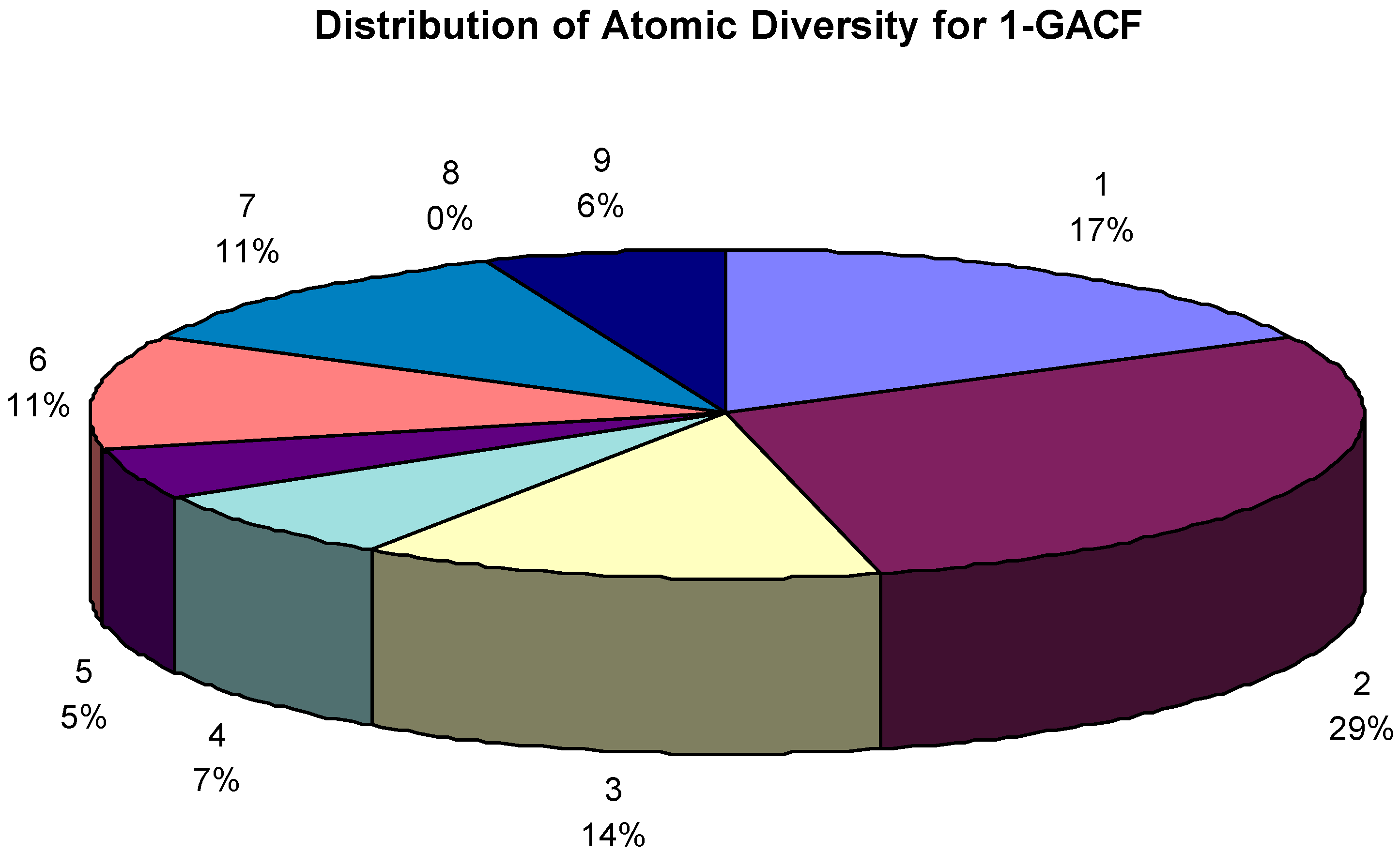
Total 64,307 GACF (General Atom Center Fragment, 1-GACF means the first layer of GACF, so and so forth) substructures (up to 2 layers) extracted from 565,513 assigned chemical shifts. The GACF class distribution is shown in Figure 9. Different GACF reflects a carbon atom with a different core structure and chemical environment; therefore Figure 9 shows the atomic diversity.
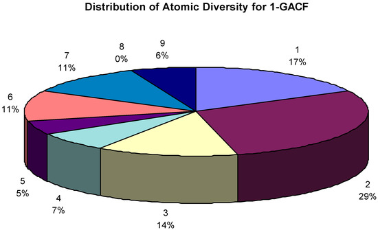
Figure 9.
The GACF class distribution. The number over the percentage figure is the code of a GACF class (refer to Table 1.). The largest portion of this knowledge body is regarding fused non-aromatic carbon atom chemical shifts. 0% actually means <1% (due to the poor resolution of the graphic display).
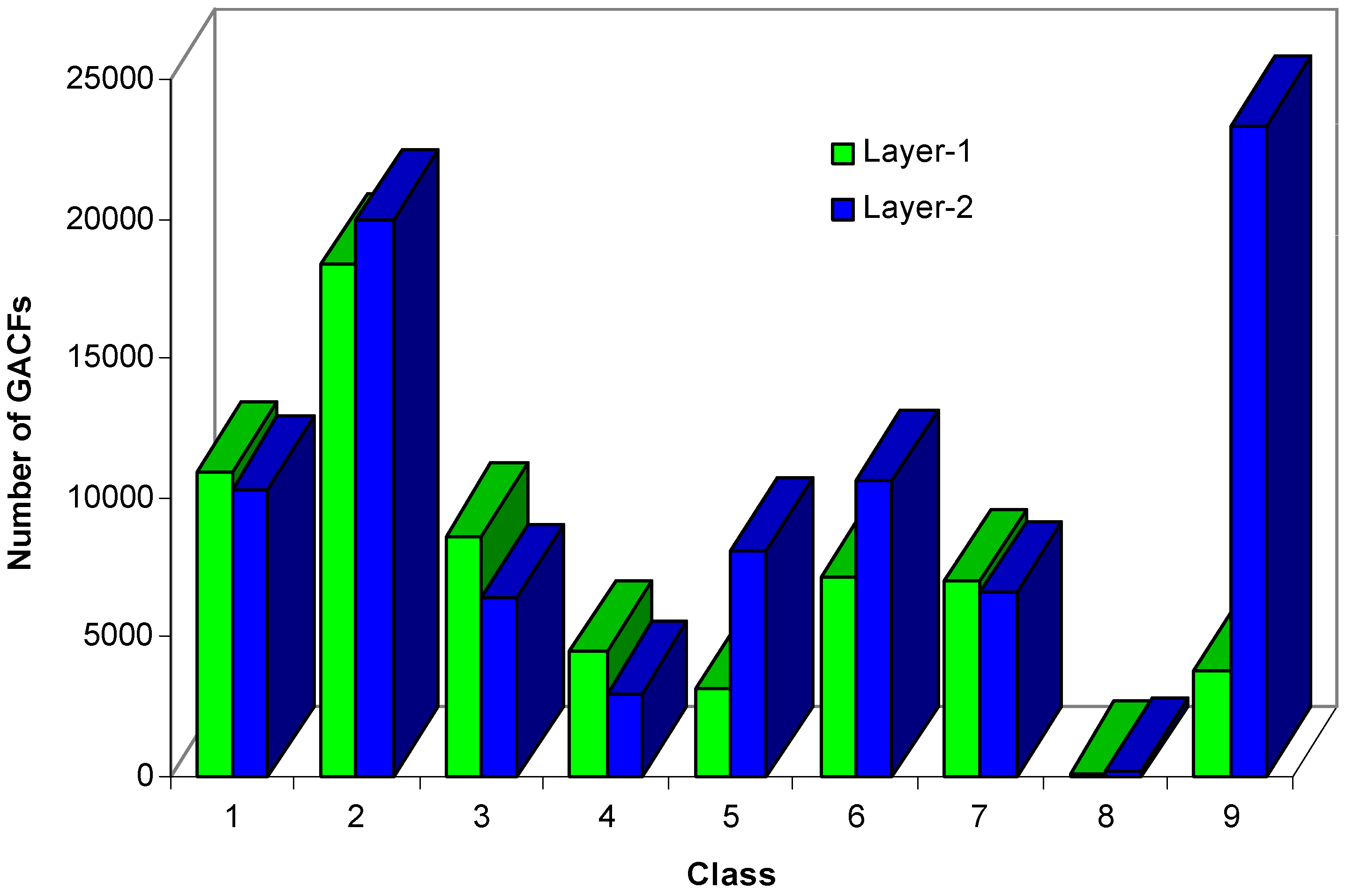
It is known that larger numbers of atom-layers will increase the size of a substructure, the size of the knowledge body, and the accuracy of the NMR spectral prediction. But, too large a knowledge body will reduce the search performance. The larger size of the GACF has less chance to be matched; that is, the knowledge will not be used very often. Figure 10 shows that 2-GACF (each GACF substructure has 2-atom-layer chemical environment) knowledge body has significantly more knowledge entries in classes 9, 5 and 6, and less entries in classes 1, 3, 4, and 7. We generate 0~2 GACF substructures for 13C NMR knowledge base, where 0-GACF substructures have only core atoms, no environmental atoms.

Figure 10.
Comparison of the sizes of 1-GACF knowledge body and 2-GACF knowledge body.
13C NMR knowledge body is the correlation table of GACF substructures and 13C chemical shifts. Its format is shown in Table 2 with an example. The "shift" is the chemical shift average value, "median" is the middle value in this range, "maximum" and "minimum" define the variable range (band). "σ" is the standard deviation, an "fn" is the number of sample chemical shifts which are used to produce the chemical shift average value, also called "frequency number".
Table 2.
The Format of GACF-Chemical Shift Correlation Table
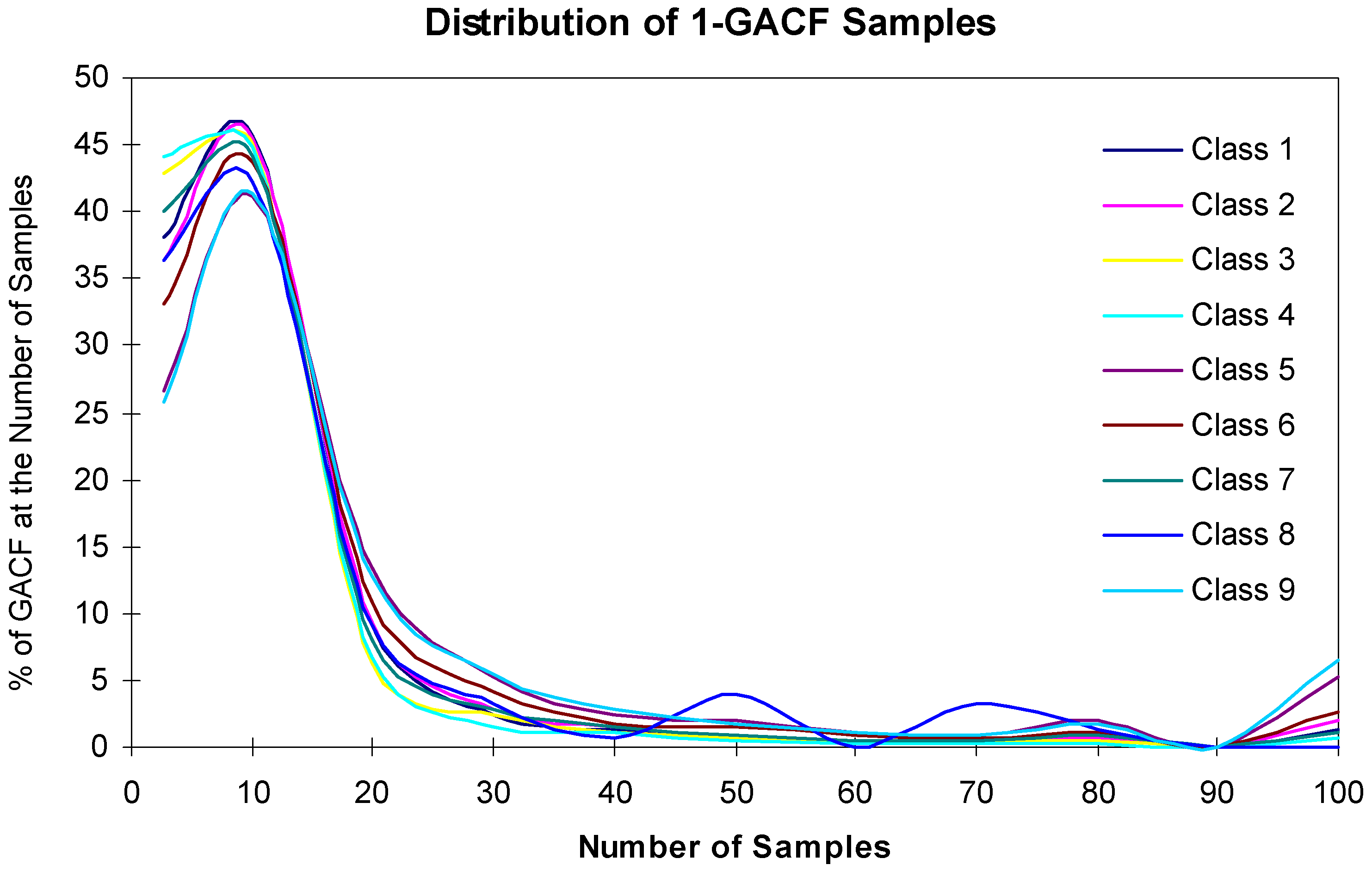
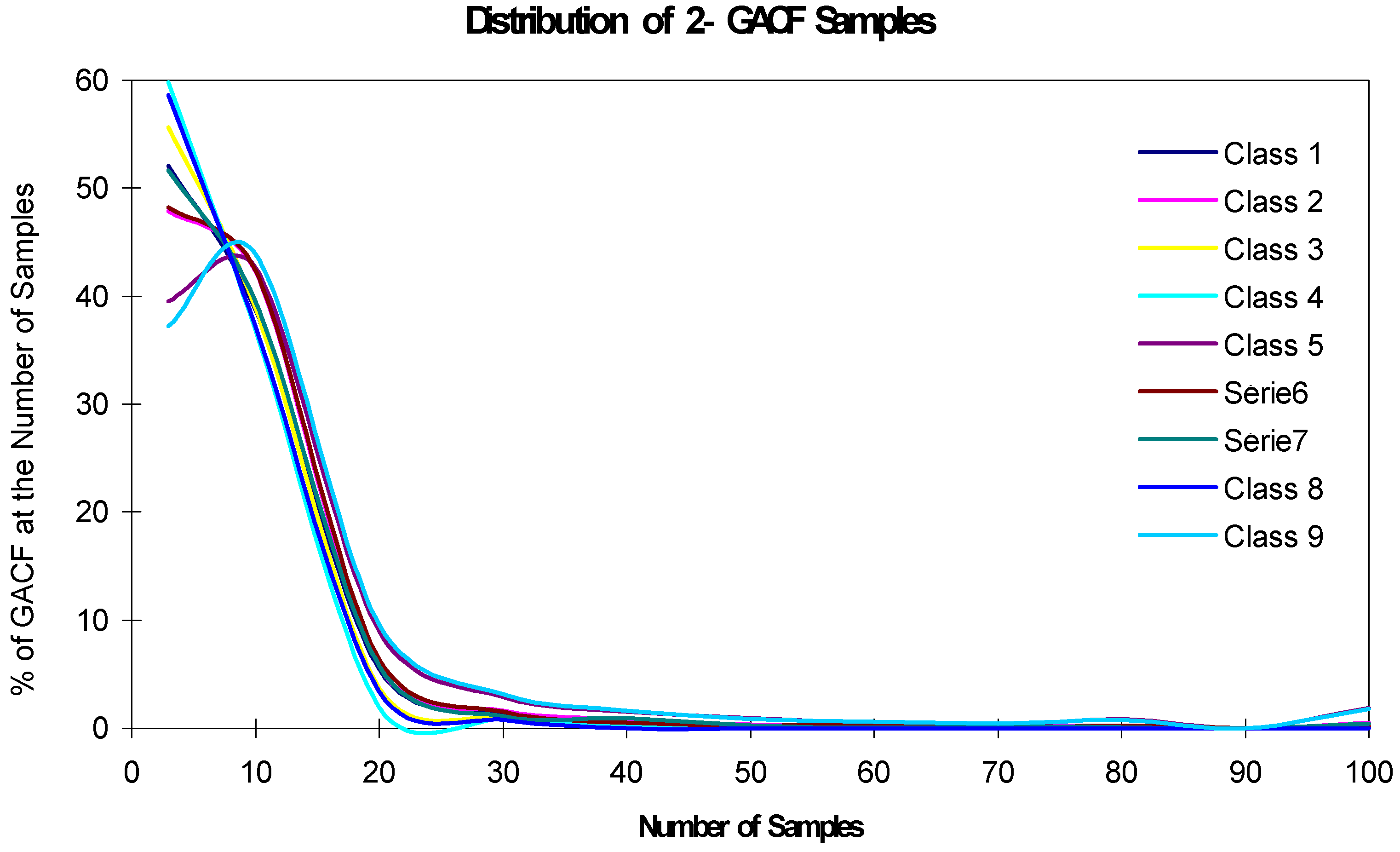
The accuracy and generality of the 13C NMR spectral prediction can be analyzed by studying the distributions of frequency numbers (fn). As shown in Table 2, fn should be larger than 3 to make statistical sense; however, if fn is too large, such as >1000, the accuracy will decrease. On the other hand, a 13C NMR KB rule with larger fn may mean that it covers larger structural diversity, and therefore, has better generality. The accuracy and generality are conflicting, and have to be balanced. Figure 11 and Figure 12 show the relationship of the fn distribution, accuracy and generality, where "the Number of Samples" is fn.
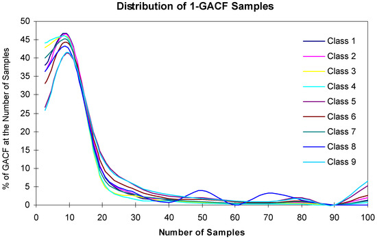
Figure 11.
Distribution of 1-GACF fn.
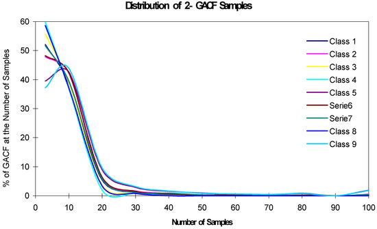
Figure 12.
Distribution of 2-GACF fn.
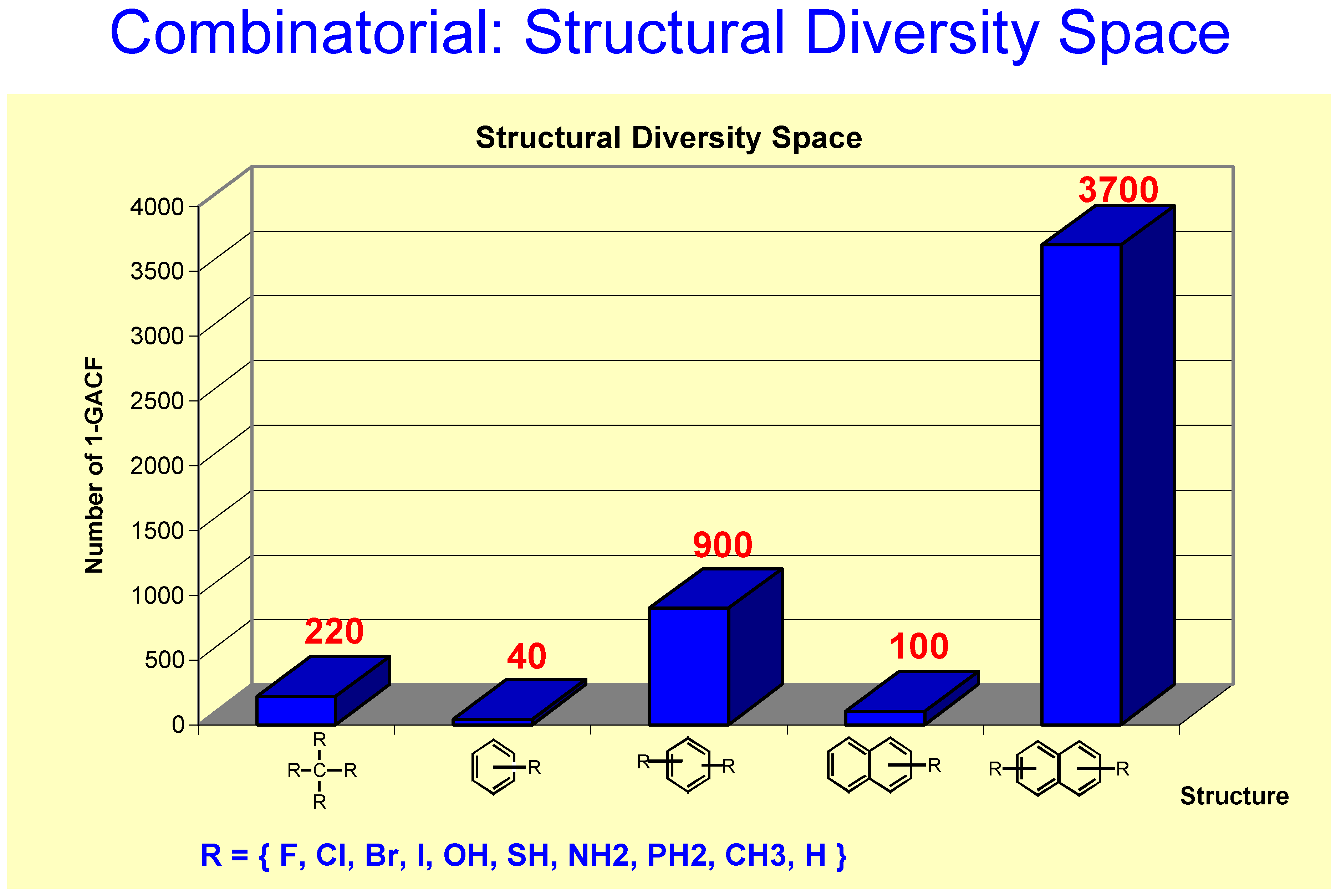
In Figure 11, about 47% 1-GACF rules have ~10 sample chemical shifts (fn). However, as shown in Figure 12, about 60% 2-GACF rules have 3~5 sample chemical shifts. Hence, 2-GACF rules will give more accurate predictions, but cover less structural diversity. In fact, the structural diversity space is extremely huge. It is almost not possible to build a knowledge base to cover the whole structural diversity with reasonable predicting accuracy. Figure 13 shows a way to estimate structural diversity space.
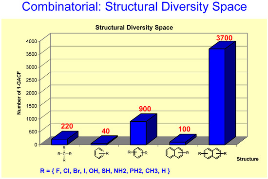
Figure 13.
If R is defined as a 10-substitute group, the number of different types of carbon atoms is 220 (1-GACF substructures), for mono-substituted benzene, it is 40 due to symmetry, 900 for disubstituted benzene, etc. This Figure shows that the structural diversity space is a “combinatorial explosion” even if the scaffolds are simple and small.
The 13C NMR spectral prediction for a given structure is described in the following steps:
- input a structure (draw a structure through a graphic user interface)
- for each carbon atom, extract a 2-GACF (2 level GACF) substructure from the structure
- search the 2-GACF against 2-GACF 13C NMR KB
- if this 2-GACF is found from the 2-GACF KB, the carbon’s chemical shift is predicted
- if not:
- extract a 1-GACF (1 level GACF) substructure from the structure
- search the 1-GACF against 1-GACF 13C NMR KB
- if this 1-GACF is found from the 1-GACF KB, the carbon’s chemical shift is predicted with less accuracy
- if not report: “cannot predict chemical shift for this type of carbon atom”
- go to 2
Searching a GACF from 64,307 GACF substructures by means of atom-by-atom search will be time-consuming. Hence, all GACF substructures have been converted to hash codes and sorted. Therefore, the GACF structure search is very fast.
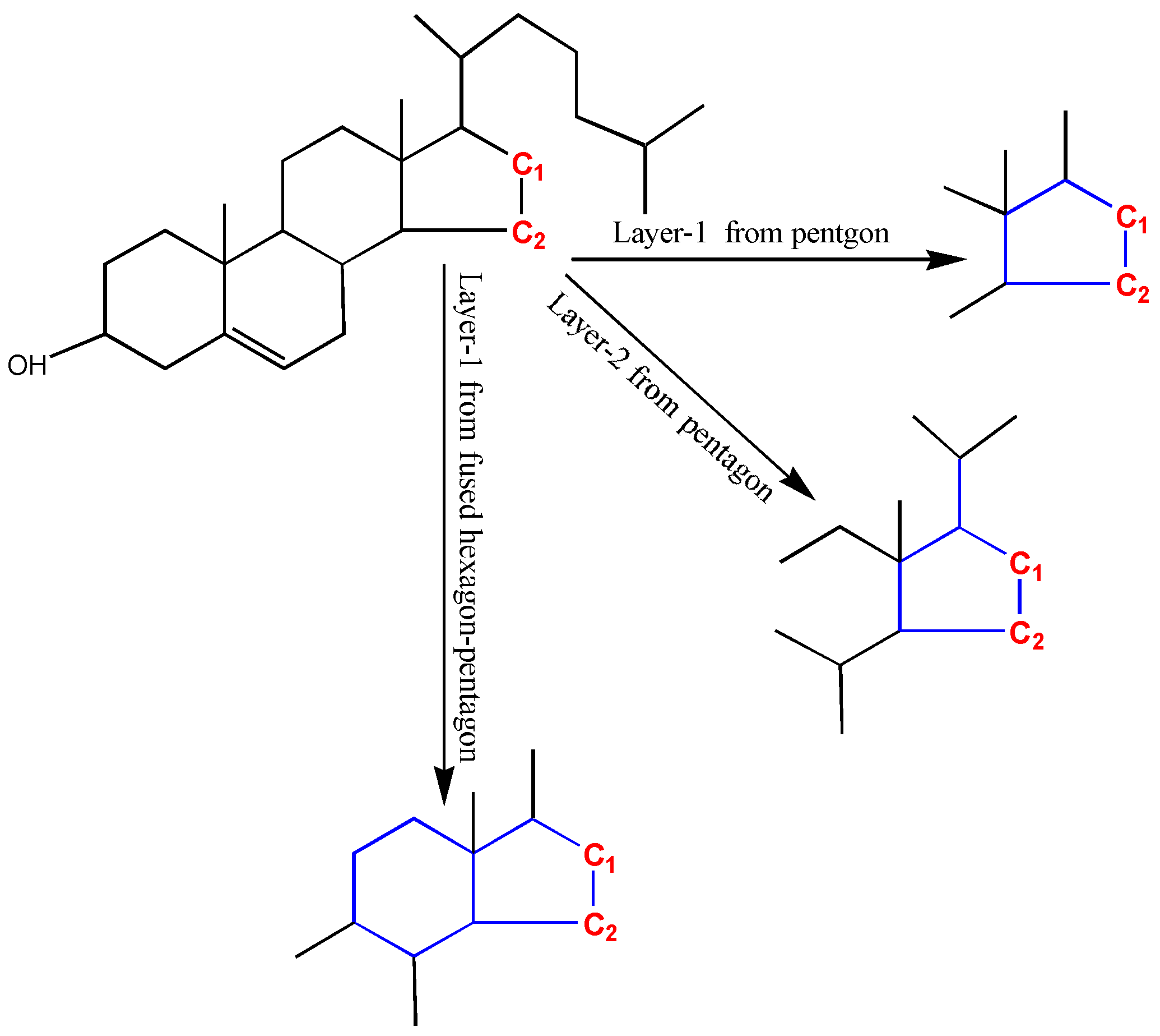
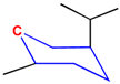
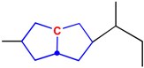
The accuracy and generality are conflicting. Discriminating similar substructures can enable more predicting accuracy, but less substructures can match the GACF in the knowledge base. In Figure 14, C1 and C2 (colored in red) should have very different chemical shifts. Taking pentagon atoms (colored in blue) as the core layer (superatom center), either 1-bond-away or 2-bonds-away from the pentagon ring, C1 and C2 cannot be distinguished. In order to distinguish C1 and C2, the fused hexagon and pentagon atoms are taken as the super-atom center. With this GACF measure, C1 and C2 are distinguished in 1-GACF.
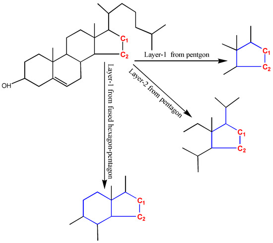
Figure 14.
C1 and C2 have very different chemical shifts (C1: 40 ppm, but C2: 24 ppm). In order to predict correctly, the substructure measurement should distinguish them. Topologically, if the pentagon is considered as core layer, C1 and C2 cannot be distinguished up to the second layer. But, if the fused hexagon-pentagon is measured as the core layer, C1 and C2 can be distinguished. The hexagon is encoded as remote fused ring in GACF substructure measurement scheme.
More discrimination, however, reduces generality. No matter how large the knowledge body is, many substructures are still not included. The mission of a prediction algorithm is to output the best estimation based upon existing knowledge collection.
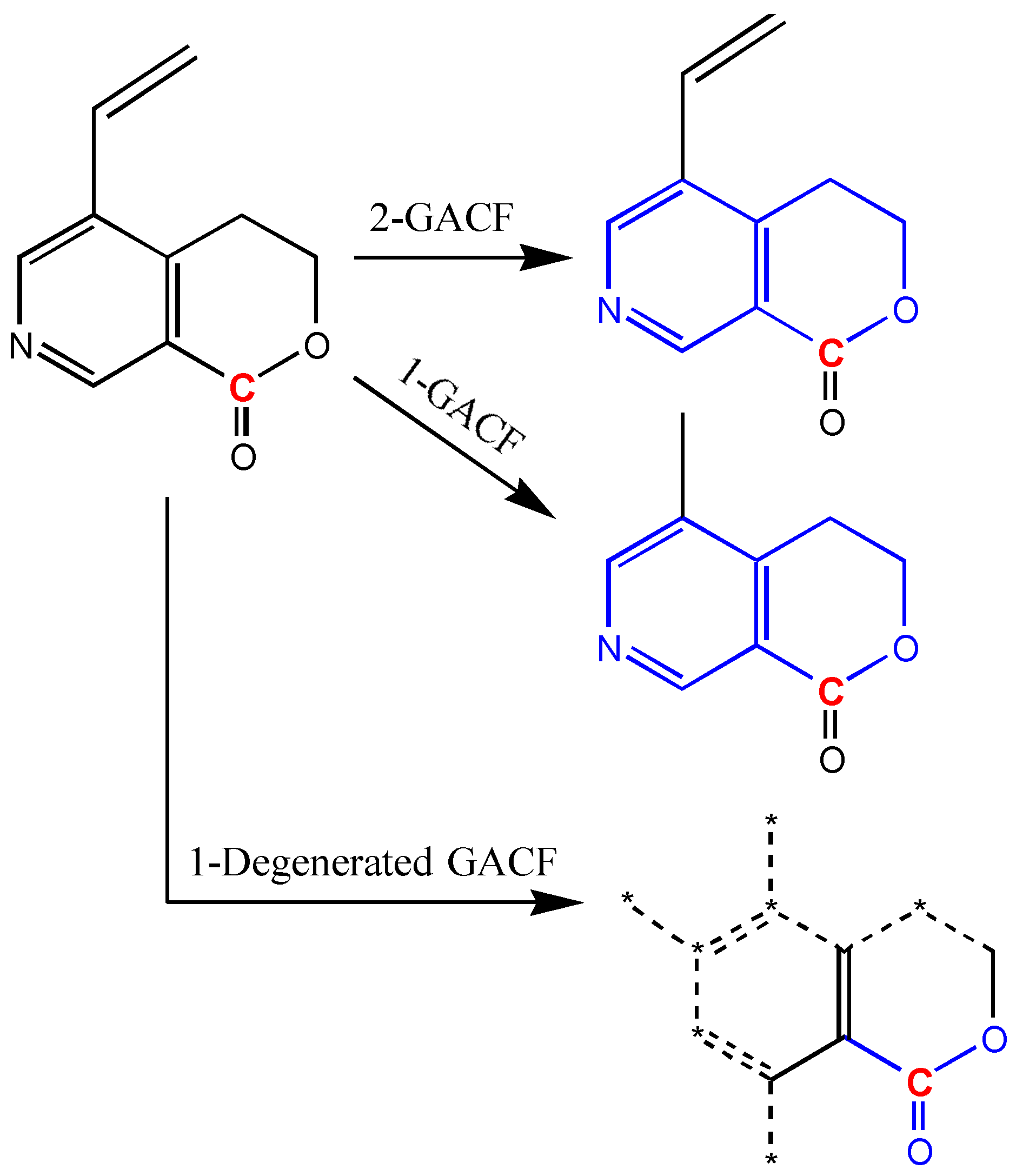
In order to compromise the accuracy and generality, degeneracy technique (way to loosen structural pattern match restriction) is introduced. If a GACF substructure is not found in a higher level GACF knowledge base, this substructure can be degenerated to become a simplified GACF, and enable more chance to match. Figure 15 shows a way to degenerate a GACF substructure.

Figure 15.
If 1-GACF and 2-GACF are not found in a knowledge base, the 1-Degenerated GACF may have more chance to match with a GACF in the knowledge base to get the closest estimation. “*” represents any atom; dashed bonds represent the bonds not in the Degenerated GACF.
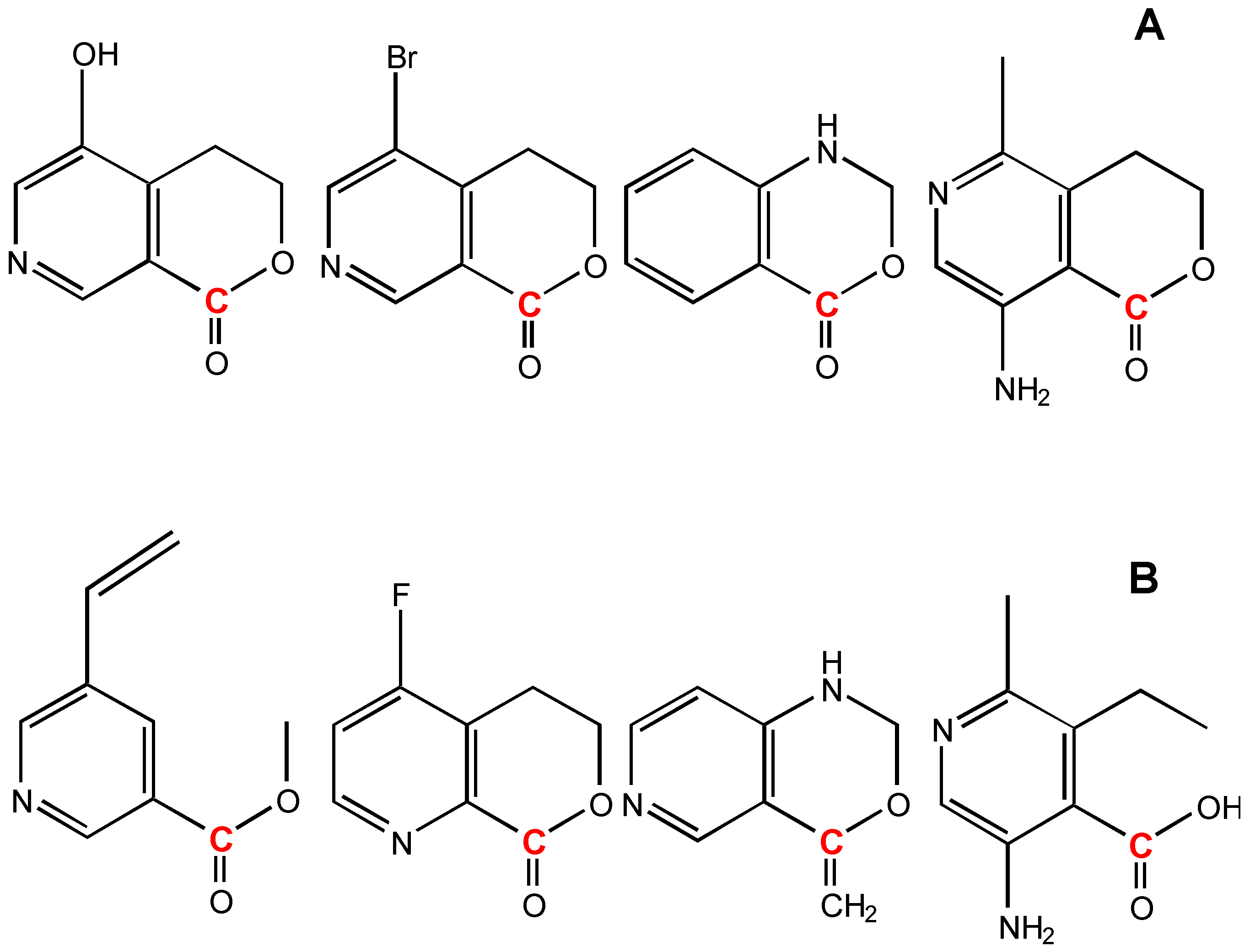
The degeneracy technique gains more generality for a knowledge base. Figure 16 A lists a set of structures used to estimated the carbon atom (colored in red) chemical shift of the 1-Degenerated GACF in Figure 15. Figure 16 B shows the structures not used for this estimation.
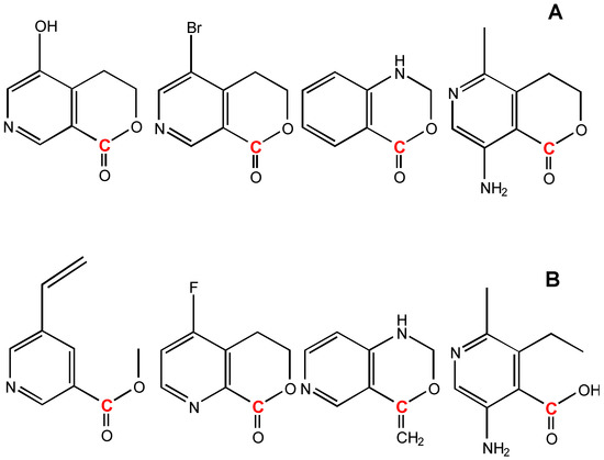
Figure 16.
A: structures used to estimate the carbon atom (colored in red) chemical shift of 1-Degenerated GACF in Figure 15. B: structures which cannot be used for this estimation.
Results and conclusions
GACF-based 13C NMR spectral prediction program has been implemented in C and Visual C++ in both UNIX (SUN or SGI) and NT/Windows platforms. The Knowledge Base occupies ~4 MB space. Average standard deviation of the prediction is 4.56 ppm. The average prediction time for a small structure (<255 carbon atoms) is less than a second. The program has been tested on a number of structures selected from other data resource by a third part chemist. Some of the testing results are listed in Table 3 for comparison.
Table 3.
Comparisons of observed chemical shift values, ACD/CNMR predictions and GACF predictions.
General speaking, KB-based NMR spectral prediction is influenced by the following factors:
- algorithms to correctly classify the center atoms and their chemical environment
- the quality of the structures-spectra database
The atomic chemical environment classification includes: (1) aromatic and non-aromatic, (2) cyclic and acyclic, (3) hetero-ring and homo-ring, (4) ring size, (5) ring types, such as single, fused, bridged, spiro, (6) saturated and unsaturated, (7) conjugated and nonconjugated, and (8) atom layers. These classifications require a set of structural perception algorithms, which have been solved in this paper.
The quality of the structures-spectra database consists of three aspects: (1) number of assignments for a atom center fragment; (2) structural diversity of the database; and (3) correctness of the database. In order to improve the prediction, we have developed tools to review the general atom center fragments, to analyze the atomic diversity of the structure database, and to correct wrong assignments. These will be discussed in a separate paper later.
References
- Pretsch, E.; Simon, W.; Seibl, J. Tables of Spectral Data for Structure Determination of Organic Compounds, 2nd Ed. ed; Springer Verlag: Berlin Heidelberg, 1989. [Google Scholar]
- Clerc, J. T.; Sommerauer, H. Anal. Chim. Acta 1977, 95, 33.
- Small, G. W.; Jurs, P. C. Analy. Chem. 1984, 56, 1314.
- Schweitzer, R. C.; Small, G. W. J. Chem. Info. Comput. Sci. 1996, 36, 310.
- Mitchell, B. E.; Jurs, P. C. J. Chem. Info. Comput. Sci. 1996, 36, 58.
- West, G. M. J. J. Chem. Info. Comput. Sci. 1993, 33, 577.
- Kvasnicka, V.; Skelenak, S.; Pospichal, J. J. Chem. Info. Comput. Sci. 1992, 32, 742.
- Anker, L. S.; Jurs, P. C. Anal. Chem. 1992, 64, 217.
- Bremser, W. Anal. Chim. Acta 1978, 103, 355.
- Robein, W. Mikrochim. Acta 1986, 2, 271.
- Chen, L.; Robien, W. Chemom. Intell. Lab. Syst. 1993, 19, 217.
- Dubois, J. E.; Carabedian, M.; Dagane, I. Anal. Chim. Acta 1984, 158, 217.
- Panaye, A.; Doucet, J.-P.; Fan, B. T. J. Chem. Info. Comput. Sci. 1993, 33, 258.
- Munk, M. E.; Lind, R. J.; Clay, M. E. Anal. Chim. Acta 1986, 184, 1.
- Xu, J. J. Chem. Inf. Comput. Sci. 1996, 36, 25.
- Sample Availability: not available.

© 1997 MDPI. All rights reserved