Entropy-Based Application Layer DDoS Attack Detection Using Artificial Neural Networks

Abstract

Distributed denial-of-service (DDoS) attack is one of the major threats to the web server. The rapid increase of DDoS attacks on the Internet has clearly pointed out the limitations in current intrusion detection systems or intrusion prevention systems (IDS/IPS), mostly caused by application-layer DDoS attacks. Within this context, the objective of the paper is to detect a DDoS attack using a multilayer perceptron (MLP) classification algorithm with genetic algorithm (GA) as learning algorithm. In this work, we analyzed the standard EPA-HTTP (environmental protection agency-hypertext transfer protocol) dataset and selected the parameters that will be used as input to the classifier model for differentiating the attack from normal profile. The parameters selected are the HTTP GET request count, entropy, and variance for every connection. The proposed model can provide a better accuracy of 98.31%, sensitivity of 0.9962, and specificity of 0.0561 when compared to other traditional classification models.

1. Introduction

On 31 August 2016, there was news of a recent attack with the headline “Rio 2016 Olympics suffered sustained 540 Gbps DDoS attacks”. These cyber-attacks from anonymous hackers across the globe are successful in targeting websites which even include the federal government’s official website for Rio Olympic 2016 and Brazilian Ministry of Sports. These attacks started several months before the game, and most of them were able to succeed due to the unpreparedness of the defenders. To carry out an attack on the server and deny service to other normal users, either a system or a group of systems simultaneously transmit an enormous amount of traffic to the server. The server cannot respond to the massive traffic, and therefore it denies services to benign clients or, in the worst case, even crashes. When this is achieved by a single system, we refer to it as a denial-of-service (DoS) attack [1]. When numerous systems are involved to achieve the same goal from different geographical areas, we refer to it as a distributed denial-of-service (DDoS) attack [2].

The system should be installed with an automated program to carry out the attack; this is made possible through system vulnerabilities [3], use of bot dropper [4], etc. Droppers are a piece of malware that bypass system defenses to implant a bot on other systems. Another form of recruiting bots includes inserting malicious code inside unauthorized software or as mail attachment and luring the clients into downloading it. Once the software is downloaded and installed, the malicious program is installed automatically and receives their updates from the command and control (C&C) server handled by the attacker. We refer to such an infected system used by the hacker to bring down a server as a bot, and the network of bots at different geographical areas as botnet [2]. DDoS attacks are major cybercrimes in the present society, with motives being enmity, ransom, hatred, competitions, political affairs, etc. [5,6].

Depending on the nature of the attack, we broadly classify DDoS attacks into a layer three or four DDoS and a layer seven DDoS attack [7]. Layer three or four attacks consume server bandwidth and are caused by manipulation of the working of layer three or four protocols, such as Internet control message protocol (ICMP), Synchronize sequence numbers (SYN), transport control protocol (TCP), user datagram protocol (UDP) [8], etc. A layer seven attack uses the open systems interconnection (OSI) and layer seven protocols such as hypertext transfer protocol (HTTP), domain name service (DNS) [8], etc. Application-layer DDoS attacks are hard to handle and detect as they can easily bypass the intrusion detection system (IDS) or intrusion prevention system (IPS). This attack uses genuine protocols to knock down the server either by exhausting the server resources or bandwidth [9].

In this paper, we describe how to detect application-layer DDoS attacks by computing the entropy of HTTP GET request count per connection, the variance of the entropy per IP address, and the number of HTTP GET request counts. We implemented a multilayer perceptron with genetic machine learning algorithm (MLP-GA) to classify an attack from normal clients. The objective of the use of a classification model is to accurately predict the class of the participating clients after analyzing the data. Another objective of the paper is to show that the entropy value decreases in cases of an attack. We also conclude that the nature of the packet transmission from an attack source is almost identical, as every source node is deployed with an automated program.

The rest of the paper is organized as follows. Section 2 describes the related works done. Section 3 describes the background of our approach to detect the application-layer DDoS attacks and the classification models, along with the computed data to validate the model. In Section 4, experimental setups and analysis are presented. Finally, Section 5 provides the conclusion and points out future work.

2. Related Works

A quantitative-based DDoS attack model for analyzing the DDoS detection schemes is proposed [10]. Two important factors used for detection were identified. The first factor is the proportion of the compromised clients that has the capability to access the victim. The second factor is the effect of the compromised clients on all the clients accessing the victim server. A traffic-monitoring point is set up to observe the state of the traffic, which is made possible through the concept of network traffic state (NTS). The Joint Deviation Rate metric is used to describe the deviation of the network traffic state. However, the paper does not consider the scenario where the monitoring point itself becomes the victim of the attack.

Detection and mitigation of known and unknown DDoS attacks in real-time environment using artificial neural network (ANN) are proposed [11]. The author used a training ANN algorithm to detect DDoS attacks based on distinct patterns, where it prevents DDoS-attacking traffic from reaching the target, but allows genuine traffic to pass through. Topological ANN structures such as TCP, ICMP, and UDP are specified, each having three layers (input, hidden, and output layers). The number of nodes in each topological structure is different. Hidden nodes deal with the computation process concerning input and output nodes. The output layer consists of one node to represent 1 (attack) and 0 (genuine traffic). However, if the system generates an output value of 2, traffic is unidentified by the ANN. As a solution to that, ANN needs to retrain using an up-to-date dataset.

Detection of a DDoS attack against a data center using correlation analysis is proposed [12]. It makes use of the correlation information of flow in the data center. The author provides a mechanism based on K-nearest neighbor with correlation (CKNN) and r-polling model to reduce the overhead due to the density of the training dataset. One of the important uses of the CKNN model is that it is suitable to classify network traffic even with a high noise signal.

A fuzzy estimator-based model [13] is proposed, not only to identify DDoS attacks, but also to detect offending IP addresses. It takes mean packet arrival time as the primary input metric. In the detection phase, the mean packet arrival for each IP address is compared with the fuzzy estimator. In the case of an attack, the computed value of the mean packet arrival time will not fit a Poisson description. The fuzzy estimator has an accuracy above 80%. When considered for the Defense Advanced Research Projects Agency (DARPA) dataset it has an accuracy of almost 99%. Depending on the datasets chunk, the fuzzy estimator provides an accuracy of 3/5, 5/5, and 5/6, which on average yields 81%.

Vulnerabilities in the use of entropy for DDoS attack detection have been proposed [14]. The paper used entropy to measure the amount of disorder in the data observed. It further states that entropy could be spoofed so that it remains in an expected range to raise a false positive in detection. However, in our work, we used entropy to measure the amount of disorder in the flow of the packets or request in the form of an HTTP GET request at multiple time slots. This work does not maintain a fixed range for entropy, so spoofing of packets will not create a problem. In our paper, we concentrate only on an application-layer DDoS attack caused by a protocol such as the HTTP GET request.

DDoS attack detection based on the browsing order of webpages had been proposed [15]. The authors used correlation with time of browsing to the size of the webpage information for classifying the attack from that of the normal profile.

Verification using CAPTCHA (completely automated public Turing test to tell computers and humans apart) [16] has been treated as one of the best-known mechanisms for mitigating application-layer DDoS attack. However, due to the frequent use of CAPTCHA for every webpage requested, clients became annoyed. This mechanism consumes large bandwidth and will be the bottleneck to the system itself.

A ScoreForCore [17] mechanism was introduced for DDoS attack detection and filtering. It is based on the score value which is calculated for each incoming packet; the mechanism then decides whether it is legal or not. In the ScoreForCore method, the input attributes used are IP address, port number, protocol type, packet size, time to live (TTL) value, and TCP flag.

Two submodule DDoS detection and mitigation techniques were proposed [18]. The first module is the detection stage that utilizes the Institute of Electrical and Electronics Engineers (IEEE) 802.11 distributed coordination function (DCF) standard and two-dimensional Markov chain. The second module is the mitigation of the DDoS attack using a cross-layer design technique.

3. Background

3.1. Attack Scenario

A layer seven DDoS attack on a web server is carried out by multiple abnormal clients sending massive HTTP GET requests to the web server. There are some cases when multiple normal clients transmit a huge HTTP GET request, but this could not be treated as DDoS attack. The difference between the above two cases is that in the second case, there is no particular order of the flow. There can be a high value and low value of the flow count at different instants of time. A normal client or human client accessing the web server in a random fashion results in the number of HTTP GET request counts being random. However, in the case of an attack, the clients are equipped with the automated program and, therefore, transmit an HTTP GET request in a particular fashion to overwhelm the web server. Figure 1 provides a typical DDoS attack scenario.

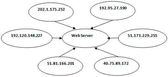
Figure 1. Attack scenario.

To overwhelm the web server, the attacker sends a large number of requests. In this work, the randomness of the flow is shown by computation of entropy. A smaller value of entropy will demonstrate that the flow is in order, otherwise the flow is out of order. In the case of an attack, the mean entropy value will be small when compared with a normal scenario.

In the paper, we consider the IP addresses 51.81.166.201 and 192.95.27.190 in Figure 1 as normal clients, while the rest are attacking clients. In Figure 1, we show only six IP addresses for easier and faster analyzing of the attack and normal scenario. The total number of clients considered for accessing the web server is 357. Each attack client is installed with an automated program to send a massive HTTP GET request. The details of experimental setup are described in Section 4. We consider and analyze the HTTP GET request, the entropy, and the variance for each IP address during a period of time.

3.2. Features Selected

In this work, we analyzed the dataset generated by a live DDoS attack obtained through experimental setup and standard EPA-HTTP (environmental protection agency-hypertext transfer protocol) datasets [19]. From the analysis of datasets, it is observed that number and characteristics of HTTP GET requests play an important role in differentiating the nature of the web-accessing clients. The important characteristics include the entropy of the HTTP GET request flow at different time intervals and variation in the flow.

From the analysis of the EPA-HTTP dataset we consider the following assumptions:

• DDoS attack from most of the attackers to a single target server occurs for at least 20 s.
• During the attack period, the attackers send HTTP at an almost constant high rate.
• Legitimate human clients could not access the web server in a constant fashion, i.e., the HTTP flow rate from a normal client is often random.

3.2.1. HTTP GET Request Count

HTTP is an important application-layer protocol used for hypertext document exchanges [20]. The operation of HTTP starts with a client by sending a request to the server in the form of a request method, uniform resource identifier (URI), and version of the protocol, followed by a multipurpose internet mail extension (MIME). On receiving the request from the client, the server responds with a status line, including the message’s version of the protocol used and a code indicating error or success, followed by a MIME. There are various methods in HTTP such as GET, POST, PUT, DELETE, HEAD, CONNECT, TRACE, and OPTIONS, which are used for the communication. In this context, we consider the HTTP GET request. We count the number of HTTP GET requests for a particular connection within a time window of 20 s. We consider 20 s as the time window since most of the automated tools (like Slowloris, High Orbit Ion Cannon (HOIC) [21], Low Orbit Ion Cannon (LOIC) [21], etc.) are programmed to bring down a web server within this time period.

We count the number of HTTP GET requests for a particular IP address by making a time slot of 20 s. The analysis is made possible by installing a Wireshark [21] at the targeted web server. Algorithm 1 provides the steps for counting the number of HTTP GET requests.

In Algorithm 1, $\mathrm{Frame}.{\mathrm{Time}}_i$ indicates the i-th time at which the packet capture starts. We denote the start time by strx (in s). ${\mathrm{IP}}_j$ denotes the j-th IP address of the participating client and ${\mathrm{IP}}_{\mathrm{dst}}$ refers to the IP address of the victim server. ${\mathrm{H}}_{\mathrm{GET}}$ indicates the selection of only the HTTP GET request. Therefore, the computed value of Final gives total flow count of HTTP GET requests for a j-th client during a 20 s time window.

Table 1, Table 2, Table 3, Table 4 and Table 5 show the captured flow count during the first timeframe window up to the fifth window respectively. It also shows the connection between source IP address and the destination IP address. For this paper, we picked up the best six connections for demonstration.

Table 1. Flow count for the first 20 s time window.

Number	Source Address	Destination Address	Flow Count
1	202.1.175.252	71.126.222.64	1213
2	192.120.148.227	71.126.222.64	1242
3	51.81.166.201	71.126.222.64	221
4	192.95.27.190	71.126.222.64	1856
5	51.173.229.255	71.126.222.64	739
6	40.75.89.172	71.126.222.64	1182

Table 2. Flow count for the second 20 s time window.

Number	Source Address	Destination Address	Flow Count
1	202.1.175.252	71.126.222.64	619
2	192.120.148.227	71.126.222.64	637
3	51.81.166.201	71.126.222.64	78
4	192.95.27.190	71.126.222.64	1025
5	51.173.229.255	71.126.222.64	322
6	40.75.89.172	71.126.222.64	600

Table 3. Flow count for the third 20 s time window.

Number	Source Address	Destination Address	Flow Count
1	202.1.175.252	71.126.222.64	1229
2	192.120.148.227	71.126.222.64	1278
3	51.81.166.201	71.126.222.64	301
4	192.95.27.190	71.126.222.64	1803
5	51.173.229.255	71.126.222.64	217
6	40.75.89.172	71.126.222.64	1201

Table 4. Flow count for the fourth 20 s time window.

Number	Source Address	Destination Address	Flow Count
1	202.1.175.252	71.126.222.64	1253
2	192.120.148.227	71.126.222.64	1273
3	51.81.166.201	71.126.222.64	334
4	192.95.27.190	71.126.222.64	1734
5	51.173.229.255	71.126.222.64	77
6	40.75.89.172	71.126.222.64	1099

Table 5. Flow count for the fifth 20 second time window.

Number	Source Address	Destination Address	Flow Count
1	202.1.175.252	71.126.222.64	1236
2	192.120.148.227	71.126.222.64	1277
3	51.81.166.201	71.126.222.64	377
4	192.95.27.190	71.126.222.64	1713
5	51.173.229.255	71.126.222.64	116
6	40.75.89.172	71.126.222.64	1148

Algorithm 1 HTTP GET Flow Count for the N Participating Clients for Every 20 s Time Window

1: Begin

2: for ($\mathrm{Frame}.{\mathrm{Time}}_i=\mathrm{strx};\mathrm{Frame}.{\mathrm{Time}}_i<\mathrm{Frame}.{\mathrm{Time}}_i+20;i++$)

3:   for (${\mathrm{IP}}_j=1;{\mathrm{IP}}_j\le \mathrm{N};j++$)

4:    Compute $\mathrm{I}=\left({\mathrm{IP}}_j\&\& {\mathrm{IP}}_{\mathrm{dst}}\right)$

5:    Compute ${\mathrm{H}}_{\mathrm{GET}}=\left(\mathrm{http}.\mathrm{request}.\mathrm{method}==\mathrm{GET}\right)$

6:    Compute Final $=\mathrm{I}\&\& {\mathrm{H}}_{\mathrm{GET}}$

7:   end for

8:  end for

9: end

3.2.2. Entropy and Variance of the Connection

For every particular connection, we calculate the entropy value of the HTTP GET flow count given in Table 1, Table 2, Table 3, Table 4 and Table 5. The entropy $E_{\left(i,w_t\right)}$ for a particular connection $C_{\left(i,w_t\right)}$ within the time slot $w_t$ is given by Equation (1) [22]. The computed entropy values for the connections are given in Table 6.

$$E_{\left(i,w_t\right)}=-log\frac{C_{\left(i,w_t\right)}}{{\sum }_{i=1}^n{C}_{\left(i,w_t\right)}}+{\lambda }_{\left(i,w_t\right)}$$

(1)

where

$${\lambda }_{\left(i,w_t\right)}=\{\begin{array}{c}\left|log\frac{c_{\left(i,w_{t+1}\right)}}{c_{\left(i,w_t\right)}}\right|,c_{\left(i,w_t\right)}\ge c_{\left(i,w_{t+1}\right)}\\ \left|log\frac{c_{\left(i,w_t\right)}}{c_{\left(i,w_{t+1}\right)}}\right|,c_{\left(i,w_t\right)}<c_{\left(i,w_{t+1}\right)}\end{array}$$

Table 6. Entropy, mean, and variance values for different time windows.

Source Address	Entropy					Mean	Variance	Approximate
	First Window	Second Window	Third Window	Fourth Window	Fifth Window
202.1.175.252	1.018	1.022	0.544	0.669	0.678	0.786	0.0386874	0.039
192.120.148.227	1.006	1.014	0.521	0.657	0.663	0.772	0.0402854	0.040
51.81.166.201	1.918	2.211	1.192	1.290	1.319	1.586	0.162998	0.163
192.95.27.190	0.799	0.751	0.387	0.527	0.548	0.602	0.0139102	0.014
51.173.229.255	1.302	1.179	1.739	2.052	2.106	1.676	0.143426	0.143
40.75.89.172	1.032	1.038	0.585	0.738	0.745	0.828	0.0319508	0.032

We consider the variance of the entropy value, since the value of the variance provides the variations in the entropy value. The variance V for a particular connection $c_i$ is given by Equation (2), where M is the mean value of the entropy and N is the number of entropy value considered. The calculated values of the variance for the particular connection are given in Table 6. In case of an attack, there is an almost identical fashion of packet transmission. As a result, the variance value is close to zero when compared with the normal client scenario.

$$V=\frac{{\sum }_i^n{\left(c_i-M\right)}^2}{N}$$

(2)

3.3. Multilayer Perceptron with Genetic Algorithm Learning

In the paper, for classifying the attacker from the normal clients based on the parameters discussed above, we consider multilayer perceptron (MLP) with genetic algorithm (GA) learning [23] as the classification model. We use GA to train the MLP neural network instead of the traditional gradient descent used in back-propagation (BP) and find the correct weights of the network. The steps are shown as follows:

● Step 1: Neural Network Model

The neural network that we used is the MLP. The structure of the neural network is given in Figure 2. The network contains three layers: input layer, one hidden layer, and output layer. The layers are connected by synaptic weights.

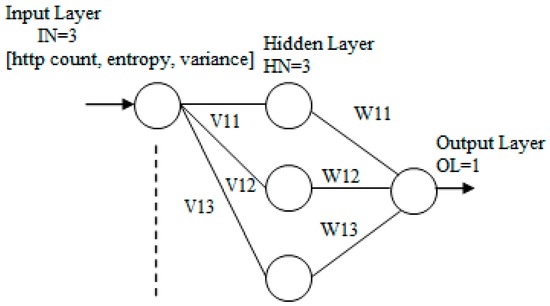
Figure 2. Structure of the multilayer perceptron (MLP) network.

In our application, the size of each input pattern is 3. The number of hidden neurons is 3. The number of output neurons is 1. The input layer consists of the combination of HTTP count, entropy, and variance, which is an attribute of the input neuron layer. The number of total weights, TW, will be given by Equation (3)

$$\mathrm{TW}=\mathrm{IN}·\mathrm{HN}+\mathrm{HN}·\mathrm{ON}$$

(3)

where IN is the size of input pattern, HN is the number of hidden neurons, and ON is the number of output neurons. In our paper, the total number of weights, TW, given in Equation (3) is 12.

● Step 2: Weights initialization

To find the correct weights of the connection of the layers of the MLP, we use GA. In the beginning, the GA randomly creates a population of complete strings called solutions or individuals. All the weights of the connection of MLP layers can be represented by each solution/individual of the GA population. The solution will be a bit string of 0 s and 1 s.

The genelength, GL, will be given by the Equation (4)

$$\mathrm{GL}=\left(\mathrm{B}·\left(\mathrm{IN}·\mathrm{HN}+\mathrm{HN}·\mathrm{ON}\right)\right)$$

(4)

where B = number of bits per weight. We represent each weight using 16 bits binary number, i.e., B = 16, then genelength, GL, from Equation (4) is 192. So, the genotype of our solution/individual is a 192 bit binary string.

● Step 3: Reconstruction of the phenotype from the genotype

After generating the solutions, we need to calculate the fitness value of each solution using a fitness equation. To calculate the fitness, we need to find the phenotype of each 16 bit substring, which represents each individual weight. The phenotype, $y_i,$ of each substring is a numeric value which is the actual value of each weight and is given by Equation (5).

$$y_i={\displaystyle \sum }_{k=1}^{\mathrm{B}}{\mathrm{b}}_{ik}{2}^{-k}$$

(5)

where, b_ik is the k-th bit of the i-th weight. The phenotype is again modified to put the weight value in some convenience range, and is given by Equation (6):

$$w_i=y_i·\mathrm{A}+\mathrm{B}$$

(6)

where $w_i$ is the i-th weight present in the string/solution, A is the scaling factor, and B is the shifting factor.

In this paper, we take the weight value from [−10,10], so we make A = 20 and B = −10 in Equation (6).

In this way, we get the weights, $v_{ij}$, which is the weight from the i-th input to the j-th hidden neuron and the weights, $w_{jk}$, which is the weight from the j-th hidden neuron to the k-th output neuron.

● Step 4: Output of the hidden layer and the output layer

Now the weights obtained will combine with the input and obtain from each layer. We get a training example x from the training set, and then calculate the outputs of the hidden neurons:

$$\mathrm{s}1={\displaystyle \sum }_{i,j}{v}_{ji}·x_{pi}$$

(7)

$$y_j=\mathrm{sigmoid}\left(\mathrm{s}1\right)$$

(8)

Using Equations (6) and (7) we calculate $y_j$, which is the output of the j-th hidden neuron.

● Step 5: Calculate the output of the output neurons

The output of the output neurons can be calculated by:

$$\mathrm{s}2={\displaystyle \sum }_{j,k}{w}_{kj}·y_j$$

(9)

$${\mathrm{o}}_k=\mathrm{sigmoid}\left(\mathrm{s}2\right)$$

(10)

where ${\mathrm{o}}_k$ is the output of the k-th output neuron. The function sigmoid ( ) is a unipolar sigmoid function given by:

$$\mathrm{sigmoid}\left(\mathrm{x}\right)=\frac{1}{1+{\mathrm{e}}^{-\mathsf{\lambda }·\mathrm{x}}}$$

(11)

These two operations of finding the output are performed for all the input patterns. Then we update the Error, E, with Equation (12) using Equations (9) and (10):

$$\mathrm{E}=\frac{1}{2}{\displaystyle \sum }_{k=0}^K{\left({\mathrm{d}}_k-{\mathrm{o}}_k\right)}^2$$

(12)

where ${\mathrm{d}}_k$ is the desired output. This process is performed until all the training samples have been used.

● Step 6: Calculate the fitness of the string/solution

The fitness of the string/solution can be calculated with the fitness definition using Equation (13).

$$\mathrm{fitness}=\raisebox{1ex}{$1-\mathrm{E}$}\!\left/ \!\raisebox{-1ex}{$\mathrm{N}$}\right.$$

(13)

where N is the number of patterns/training examples. The above processes are repeated from step 2 onward for all the strings/solutions of the population. In this paper, the generated fitness value is given in Table 7. To reduce the size of the table, we have taken the iterations that have different fitness values and omitted the any values that have same fitness value.

Table 7. Generated fitness values and comparisons with original fitness values.

Number	Iteration	Highest Fitness Value	Original Fitness Value (0.99)
1	1	0.928571	Less
2	5	0.92993	Less
3	9	0.937984	Less
4	22	0.94349	Less
5	26	0.957986	Less
6	50	0.95887	Less
7	55	0.96029	Less
8	68	0.96354	Less
9	112	0.96897	Less
10	132	0.97106	Less
11	145	0.97145	Less
12	176	0.973184	Less
13	187	0.97372	Less
14	196	0.978299	Less
15	204	0.97992	Less
16	215	0.98002	Less
17	227	0.98346	Less
18	231	0.998628	Equal

● Step 7: Selection

We find the string with the highest fitness value using Equation (13). If this highest fitness value is greater than the desired fitness value (=0.99 in our application), then the operation stops. The weights representing this string with the highest fitness value will be used for the testing/real operation phase. Table 7 shows the current fitness values at the given iterations and compares them with the original fitness values.

● Step 8: Reproduction

The population is modified using operators, namely, crossover and mutation. The above processes from step 3 onward are repeated for many generations until we get a string/solution whose fitness value is greater than or equal to the desired fitness. The weights with the highest fitness values are selected. Herein, we obtained the fitness value at the 231th iteration with the value 0.998628. The inputs to the MLP are the training populations obtained after GA optimization. The targeted outputs are the two classes, viz. attack represented by 1 and normal represented by 0. In this work, we obtained the weights of the hidden neurons and the output neurons as shown in Figure 3.

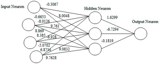
Figure 3. Weight of the hidden neuron and output neuron.

The best validation performance graph for training the input dataset is given in Figure 4. The X-axis represents the number of epoch and Y-axis represents the mean square error (mse). The best validation performance is 0.019529 at epoch 15. In Figure 4, the validation process, training process, and test error (represented by green, blue, and red lines, respectively) decrease with the increase in period of time or volume of training.

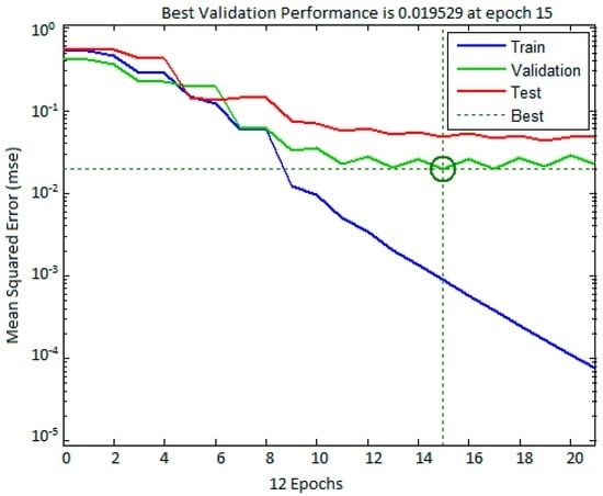
Figure 4. Validation performance graph for training the dataset.

3.4. An Illustrative Example

We consider six different inputs, each in the form of a tuple. Each tuple consists of number of HTTP flow, entropy value, and variance, respectively. The results of the operation phase for the six testing IP addresses are given in Table 8. The first column of Table 8 represents the input; the second, third, fourth, and fifth columns represents the values generated by Equations (7)–(10), respectively. The last column refers to the behavior of the packet-sending clients.

Table 8. A sample operation phase.

Input	s1	yj	s2		ok	Status
[2000,0.888,0.011]	7272.2	−1	6.22		1	Attack
[2000,4.55,4.44]	7270.9	−1	−3.74		0	Normal
[1151,0.012,0.22]	4180.5	−1	6.22		1	Attack
[1,3.33,4.77]	−5.7	−1	−3.74		0	Normal
[700,2.22,1.99]	2542.2	−1	−3.74		0	Normal
[700,0.19,0.11]	2540.8	−1	6.22		1	Attack
[400,0.001,0.022]	2122.3	−1	6.22		1	Attack
[400,5,4]	2310.7	−1	−3.74		0	Normal
[30,0.011,0.06]	−54.6	−1	6.22		1	Attack
[30,4,5]	−24.8	−1	−3.74		0	Normal

3.5. Comparison between MLP-GA with Other Classification Models

After the successful classification into either attack or normal class, we compared the classification strength of MLP-GA with that of other state-of-the-art classification models, such as MLP [24], radial basis function (RBF) network [25], naive Bayes [26], and random forest [27] in a population size of 357. We tested the accuracy of detecting the attack class and normal class, and the sensitivity and specificity of the whole population. To compare the different classifiers, we compared the receiver operating characteristic (ROC) [28] of the above-stated classifiers with MLP-GA as shown in Figure 5 and construct a confusion matrix for the given population shown in Table 9. ROC curves are plotted with X-axis representing false positive rate and Y-axis representing true positive rate using Weka 3.6 [29].

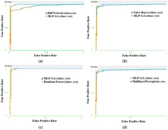
Figure 5. Comparison of receiver operating characteristic (ROC) curve of MLP-genetic algorithm (GA) with (a) radial basis function (RBF) network, (b) naive Bayes, (c) random forest, and (d) multilayer perceptron.

Table 9. Comparison for various classification models.

Classification Model	Confusion Matrix	Accuracy	Sensitivity	Specificity	Detection Time (in second)
MLP-GA	$\left[\begin{array}{cc}267\left(a\right)& 5\left(b\right)\\ 1\left(c\right)& 84\left(d\right)\end{array}\right]$	98.31	0.9962	0.0561	0.31
RBF Network	$\left[\begin{array}{cc}263\left(a\right)& 7\left(b\right)\\ 5\left(c\right)& 82\left(d\right)\end{array}\right]$	96.63	98.13	0.0787	0.53
Naive Bayes	$\left[\begin{array}{cc}165\left(a\right)& 5\left(b\right)\\ 6\left(c\right)& 81\left(d\right)\end{array}\right]$	96.92	97.79	0.0581	1.2
Random Forest	$\left[\begin{array}{cc}267\left(a\right)& 4\left(b\right)\\ 4\left(c\right)& 82\left(d\right)\end{array}\right]$	97.76	98.52	0.0465	1.6
MLP	$\left[\begin{array}{cc}260\left(a\right)& 11\left(b\right)\\ 6\left(c\right)& 80\left(d\right)\end{array}\right]$	95.23	0.9773	0.1208	0.31

To calculate the accuracy, sensitivity, and specificity from the confusion matrix for the classifiers, we use Equations (14)–(16), respectively. The comparison between the various classifier models are given in Table 10.

$$\mathrm{Accuracy}=\frac{a+d}{a+b+c+d}$$

(14)

$$\mathrm{Sensitivity}=\frac{a}{a+c}$$

(15)

$$\mathrm{Specificity}=\frac{b}{b+d}$$

(16)

Table 10. Configuration of attacks tools.

SL. No.	Tools Name	Operating System	Memory (GB)	Processors	HardDisk (GB)	Network Adapter	No. per OS
1	Slowhttptest	Red Hat 6.6	2	1	80	Bridged	1
2	LOIC	Window 8	1	1	500	NIC	4
3	HOIC	Window 7	1	1	500	NIC	3
4	R.U.D.Y	CentOS 6.8	2	1	80	Bridged	6
5	BONESI	Fedora 24	1	1	80	Bridged	1
6	Anonymous DDoSer	Window 7	1	1	500	NIC	5
7	HAVIJ	Window 8	1	1	500	NIC	5

From the comparison of the ROCs, it is concluded that MLP-GA has the perfect curve compared with the remaining classifiers.

4. Experimental Setup and Analysis

We carried out the experiments in a closed environment with a victim server and a combination of attackers and benign clients who are assessing the server. Our web server is an Apache wamp server (64 bits and PHP 5.5) 2.5 hosted on Window Operating System 7 (OS) with 8 GB RAM, 500 GB secondary memory, and Intel 7 processor. The attack tools were organized at different OS, such as Cent OS 6.8, Ubuntu 12.04, Fedora 24, Windows 7, and Window 8. To expand the number of attacker OS as well as legitimate clients, we installed at least four OS with the help of VMware Workstation version 10.0.3 in each system. We also ran at least four attack tools in each OS.

All these systems were targeting towards a common victim web server. The attack tools consisted of Slowloris attack from Slowhttptest 1.6 package, LOIC, HOIC, Anonymous DDoSer, Are You Dead Yet (R.U.D.Y), and HAVIJ, with the details given in Table 10. Havij is an SQL injection tool which employs the use of GET and POST requests. In this work, we mainly used Havij tool to make use of its GET request to the web server and not for SQL injection. Similarly, we employed R.U.D.Y tool as it makes use of HTTP POST request. To increase the number of network traffic and the number of bots, we installed botloader [30] in some of the host machines. It works on the principal of IP-aliasing to produce a large number of bots with unique IP addresses. When we ran the attack tools on the systems, the central processing unit (CPU) uses of the web server were analyzed. During the process, we found that there was a massive use of CPU resources as shown in Figure 6. Almost 88% of the CPU resources were used up during the attacking period.

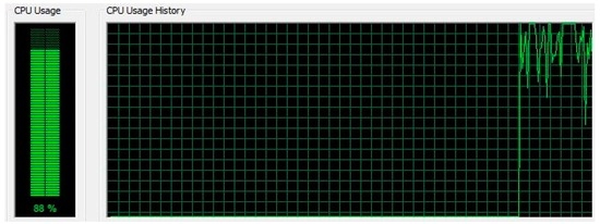
Figure 6. Central processing unit (CPU) resource utilization during attack period.

To capture all the incoming packets from different clients towards the targeted server, we installed a Wireshark of version 1.12.6 in Windows 7 OS hosting the wamp server. Wireshark as a packet analyzer can capture packets going in and out of the closed environment by adjusting the network interface card (NIC). Thus, we could get experimental log files of the DDoS attack scenario that even contained legitimate clients’ packets.

From Table 6, we observed that the mean entropy value of the third and fifth IP addresses is larger than the rest. It is concluded that for a normal client, the degree of randomness is more than that for the attack clients. This also shows that human clients normally do not have the ability to send a similar number of HTTP GET requests. The number of web requests sent during first 20 s was different from the number of requests sent afterward, whereas an attacker has the capability of sending a similar number of the requests until the web server becomes offline.

From Table 6 we also observed that the variance of the entropy for the attacking IP addresses is smaller than that of the normal clients. The variance value for the attack clients during 100 s is close to zero, which leads to the conclusion that there is much less variation in the entropy value. It is different from that of the normal clients, for which the variance of the entropy value during 100 s is large. It is concluded that a normal client has a large variation in generating the HTTP GET request.

From Table 9 it is observed that we can achieve 98.32% accuracy rate in the classification, which is more than that of simply using MLP with a back-propagation algorithm.

We used EPA-HTTP datasets for validation and verification of the methods used with live DDoS datasets. From the analysis of the dataset in Figure 7, Figure 8 and Figure 9, it is observed that attack clients have a high flow count but a lower value of entropy and variance. During flash events, the clients have a higher flow count value and higher value of entropy due to disorder in the request rate along with a higher variance value due to high variation in the flow.

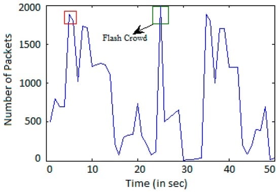
Figure 7. Hypertext transfer protocol (HTTP) count for the incoming traffic.

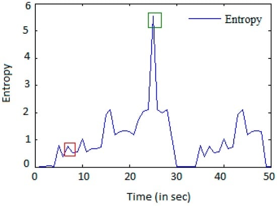
Figure 8. Mean entropy per IP address.

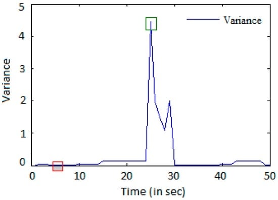
Figure 9. Variance of the entropy per IP address.

In Figure 7, Figure 8 and Figure 9, the box highlighted in red color indicates the characteristics of an attacking IP address, and the box highlighted in green color indicates the characteristics of normal clients. Considering the above assumptions, we observed that high HTTP flow is not the only criteria of identifying an attacking IP address.

An IP address having high HTTP flow rate and a high value of entropy and variance are not considered as attack clients since a high entropy value indicates that there is randomness in the transmission. A high variance value indicates that the entropy value for an IP address per 20 s varies to large extent. The green highlighted box indicates the flash events [31,32], which is a normal behavior.

Detection Time Analysis

Algorithm 2 provides the time taken by MLP-GA for detecting the nature of the clients accessing the web server.

Algorithm 2 Time Consumed by MLP-GA in Detection

Begin

Step 1: Calculate, $\mathrm{s}1={\sum }^{\text{}}\mathrm{V}·\mathrm{X}$

where X is an array of the three input attributes and V is the weight from input to hidden layers.

Step 2: Calculate, Y = Sigmoid (s1)

End

Begin

Step 3: Calculate, $\mathrm{s}2={\sum }^{\text{}}\mathrm{W}·\mathrm{Y}$

where W is the weight from the hidden to the output layers.

Step 4: Calculate, Output = Sigmoid (s2)

The value of the Output is either 0 or 1 only.

End

Step 5: if (Output = 1)

Status= Attack

Else

Status= Normal

End if

where status indicated the nature of the participating client.

GA was not involved during the testing stage. It was only used during the training stage to find the weights. Therefore, time consumed by GA is not part of the detection time. The time taken during training depends on the size of the sample and the number of the input attributes. However, training time is not part of the detection time. The detection time for 357 participating clients using different classifying models is shown in Table 9.

To carry out any DDoS attack on a target web server, the attacking clients should have constant high flow of HTTP. The duration of attack should be at least 100 s, and as a result the entropy rate for that IP address is low and only slight variations in the attacking rate occur during the attack duration. The training sets obtained from EPA-HTTP datasets were used to train the MLP-GA classification model. This model was tested against standard datasets such as CAIDA 2007 [33], DARPA 2009 [34], and BONESI-generated datasets, and the experimentally generated dataset (referred to as DATA in Figure 10). We compared the accuracy of detection in these three standard datasets by MLP-GA for a sample size of 900 as shown in Figure 10. The experimentally generated dataset (DATA) is a combination of the network traffic from multiple sources with different attack tools. The graph indicates that the accuracy of detection of DDoS attack increases with the rise in the sample size. The detection mechanism is effective for large DDoS attack datasets.

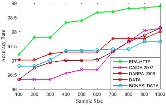
Figure 10. Accuracy curve for the proposed method.

5. Conclusions and Future Scope

In this paper, the impacts of the DDoS attacks were analyzed and important factors that influence the attack were compared. We have used a trained MLP with GA learning algorithm to detect the DDoS attack based on the number of HTTP GET requests, the entropy of the requests, and variance of the entropy. We have shown that there is higher value of entropy in the case of normal clients and lower value in the event of an attack. We have also evaluated that the amount of the variance for an attacking client is close to zero. It shows that there is not much variation in the generation of the number of HTTP GET requests during the attacking period. Our proposed approach can detect the DDoS attack with an accuracy of 98.32%, sensitivity rate of 0.9962, and specificity rate of 0.0561.

The paper is limited only to application-layer DDoS attack detection. However, its prevention mechanism is not illustrated in the paper. In future, we will extend the method to mitigate the attack on the web server by imposing fuzzy-based firewall rules to block the detected attacks. The method could be geared towards developing efficient detection for different types of DDoS attacks.

References

- Wang, B.; Zheng, Y.; Lou, W.; Hou, Y.T. DDoS attack protection in the era of cloud computing and Software-Defined Networking. Comput. Netw. 2015, 81, 308–319. [Google Scholar] [CrossRef]
- McGregory, S. Preparing for the next DDoS attack. Netw. Secur. 2013, 2013, 5–6. [Google Scholar] [CrossRef]
- Hunter, P. Distributed Denial of Service (DDoS) Mitigation Tools. Netw. Secur. 2003, 5, 12–14. [Google Scholar]
- Sood, A.K.; Enbody, R.J.; Bansal, R. Dissecting SpyEye–Understanding the design of third generation botnets. Comput. Netw. 2013, 57, 436–450. [Google Scholar] [CrossRef]
- Vissers, T.; Somasundaram, T.S.; Pieters, L.; Govindarajan, K.; Hellinckx, P. DDoS defense system for web services in a cloud environment. Future Gener. Comput. Syst. 2014, 37, 37–45. [Google Scholar] [CrossRef]
- Malecki, F. Simple ways to dodge the DDoS bullet. Netw. Secur. 2012, 2012, 18–20. [Google Scholar] [CrossRef]
- Beitollahi, H.; Deconinck, G. Tackling application-layer DDoS attacks. Procedia Comput. Sci. 2012, 10, 432–441. [Google Scholar] [CrossRef]
- Saad, R.M.A.; Anbar, M.; Manickam, S.; Alomari, E. An Intelligent ICMPv6 DDoS Fooding-attack Detection Framework (v6IIDS) Using Back-Propagation Neural Network. IETE Tech. Rev. 2015, 33, 244–255. [Google Scholar] [CrossRef]
- Ni, T.; Gu, X.; Wang, H.; Li, Y. Real-time detection of application-layer DDoS attack using time series analysis. J. Control Sci. Eng. 2013, 2013, 821315. [Google Scholar] [CrossRef]
- Wang, F.; Wang, H.; Wang, X.; Su, J. A new multistage approach to detect subtle DDoS attacks. Math. Comput. Model. 2012, 55, 198–213. [Google Scholar] [CrossRef]
- Saied, A.; Overill, R.E.; Radzik, T. Detection of known and unknown DDoS attacks using Artificial Neural Networks. Neurocomputing 2015, 172, 385–393. [Google Scholar] [CrossRef]
- Xiao, P.; Qu, W.; Qi, H.; Li, Z. Detecting DDoS attacks against data center with correlation analysis. Comput. Commun. 2015, 67, 66–74. [Google Scholar] [CrossRef]
- Shiaeles, S.N.; Katos, V.; Karakos, A.S.; Papadopoulos, B.K. Real time DDoS detection using fuzzy estimators. Comput. Secur. 2012, 31, 782–790. [Google Scholar] [CrossRef]
- Özçelik, İ.; Brooks, R.R. Deceiving entropy based DoS detection. Comput. Secur. 2015, 48, 234–245. [Google Scholar] [CrossRef]
- Yatagai, T.; Isohara, T.; Sasase, I. Detection of HTTP-GET flood Attack Based on Analysis of Page Access Behavior. In Proceedings of the IEEE Pacific Rim Conference on Communications, Computers and Signal Processing, Victoria, BC, Canada, 22–24 August 2007.
- Ko, N.-S.; Noh, S.-K.; Park, J.-D.; Lee, S.-S.; Park, H.-S. An efficient anti-DDoS mechanism using flow-based forwarding technology. In Proceedings of the 9th International Conference on Optical Internet (COIN 2010), Jeju, Korea, 11–14 July 2010.
- Kalkan, K.; Alagöz, F. A distributed filtering mechanism against DDoS attacks: ScoreForCore. Comput. Netw. 2016, 108, 199–209. [Google Scholar] [CrossRef]
- Soryal, J.; Saadawi, T. IEEE 802.11 DoS attack detection and mitigation utilizing Cross Layer Design. Ad Hoc Netw. 2014, 14, 71–83. [Google Scholar] [CrossRef]
- EPA-HTTP. Available online: http://ita.ee.lbl.gov/html/contrib/EPA-HTTP.html (accessed on 29 January 2015).
- Jestratjew, A.; Kwiecien, A. Performance of HTTP protocol in networked control systems. IEEE Trans. Ind. Inform. 2013, 9, 271–276. [Google Scholar] [CrossRef]
- Hoque, N.; Bhuyan, M.H.; Baishya, R.C.; Bhattacharyya, D.K.; Kalita, J.K. Network attacks: Taxonomy, tools and systems. J. Netw. Comput. Appl. 2014, 40, 307–324. [Google Scholar] [CrossRef]
- David, J.; Thomas, C. DDoS Attack Detection Using Fast Entropy Approach on Flow-Based Network Traffic. Procedia Comput. Sci. 2015, 50, 30–36. [Google Scholar] [CrossRef]
- Dahal, K.; Almejalli, K.; Hossain, M.A.; Chen, W. GA-based learning for rule identification in fuzzy neural networks. Appl. Soft Comput. 2015, 35, 605–617. [Google Scholar] [CrossRef]
- Yang, J.; Zeng, X.; Zhong, S. Computation of multilayer perceptron sensitivity to input perturbation. Neurocomputing 2013, 99, 390–398. [Google Scholar] [CrossRef]
- Ince, T.; Kiranyaz, S.; Gabbouj, M. Evolutionary RBF classifier for polarimetric SAR images. Expert Syst. Appl. 2012, 39, 4710–4717. [Google Scholar] [CrossRef]
- Kotsiantis, S. Integrating Global and Local Application of Naive Bayes Classifier. Int. Arab J. Inf. Technol. 2014, 11, 300–307. [Google Scholar]
- Aung, W.T.; Myanma, Y.; Hla, K.H.M.S. Random forest classifier for multi-category classification of web pages. In Proceedings of the IEEE Asia-Pacific Conference on Services Computing, Singapore, Singapore, 7–11 December 2009.
- Schubert, C.M.; Oxley, M.E.; Bauer, K.W. A comparison of ROC curves for label-fused within and across classifier systems. In Proceedings of the 7th International Conference on Information Fusion, Philadelphia, PA, USA, 25–28 July 2005.
- Jaswal, K.; Kumar, P.; Rawat, S. Design and development of a prototype application for intrusion detection using data mining. In Proceedings of the 4th International Conference on Infocom Technologies and Optimization, Noida, India, 2–4 September 2015.
- Bhatia, S.; Schmidt, D.; Mohay, G.; Tickle, A. A framework for generating realistic traffic for Distributed Denial-of-Service attacks and Flash Events. Comput. Secur. 2014, 40, 95–107. [Google Scholar] [CrossRef]
- Thapngam, T.; Yu, S.; Zhou, W.; Beliakov, G. Discriminating DDoS attack traffic from flash crowd through packet arrival patterns. In Proceedings of the IEEE Conference on Computer Communications Workshops (INFOCOM WKSHPS), Shanghai, China, 10–15 April 2011.
- Oikonomou, G.; Mirkovic, J. Modeling human behavior for defense against flash-crowd attacks. In Proceedings of the IEEE International Conference on Communications, Dresden, Germany, 14–18 June 2009.
- The CAIDA “DDoS Attack 2007” Dataset. Available online: https://www.caida.org/data/passive/ddos-20070804_dataset.xml (accessed on 20 September 2016).
- LANDER: Los Angeles Network Data Exchange and Repository. Available online: http://www.isi.edu/ant/lander (accessed on 25 May 2014).
© 2016 by the authors; licensee MDPI, Basel, Switzerland. This article is an open access article distributed under the terms and conditions of the Creative Commons Attribution (CC-BY) license (http://creativecommons.org/licenses/by/4.0/).