A Novel Numerical Method for Computing Subdivision Depth of Quaternary Schemes

Abstract

In this paper, an advanced computational technique has been presented to compute the error bounds and subdivision depth of quaternary subdivision schemes. First, the estimation is computed of the error bound between quaternary subdivision limit curves/surfaces and their polygons after kth-level subdivision by using $l_0$ order of convolution. Secondly, by using the error bounds, the subdivision depth of the quaternary schemes has been computed. Moreover, this technique needs fewer iterations (subdivision depth) to get the optimal error bounds of quaternary subdivision schemes as compared to the existing techniques.

1. Introduction

Subdivision schemes are major tools in Geometric Modeling. These tools are mainly used to produce curve and surface models. The schemes are categorized into binary, ternary, quaternary,…, n-ary schemes. Presently, thousands of schemes have been introduced in each category. All these schemes help the technologist to produce the refine models to meet the requirements of the investors in the area of engineering. The initial sketch and subdivision rules are the main ingredients of these schemes. The estimation of the error bounds of the limit models from its initial sketch is one of the important tasks. Another task is to find the number of subdivision steps (depth) required to get the user-defined tolerable error. These two tasks are also called the distance/error between the limit model & its kth level model and subdivision depth, respectively. In this paper, we address these tasks for quaternary schemes. First, we give an overview of quaternary subdivision schemes (QSS) before addressing these tasks.

In general, QSS has four rules to refine each edge of the initial polygon (sketch). These rules are the affine combination of the points of the polygon, and they produce successively refined sketches. In the limiting case, we get the limiting model. Initially, Mustafa and Faheem [1] introduced 4-point approximating QSS which produces $C^3$ models. The generalized idea of m-point approximating QSS is given by Siddiqi and Younis [2]. They also introduced interpolating QSS in the same year [3]. A 4-point QSS is presented by Pervaiz [4] in 2018. Moreover, the QSS also belongs to the classes of the schemes introduced by [5,6,7,8,9,10,11,12,13] in different years. So, the importance of the QSS cannot be denied. Furthermore, the tasks of finding the error bounds and subdivision depth of models produced by QSS are meaningful.

The first technique was introduced by Mustafa et al. [14] in 2006, then its generalized version for QSS was presented by Mustafa et al. [15] in 2010. The further generalization has also been done for other categories of the schemes [16]. This technique is not suitable to use for some subdivision schemes. We also mention the drawback of this technique in this paper. The second technique is introduced by Deng et al. [17]. It is not mature enough. It only works for binary interpolating schemes. Its generalization to the cases of n-ary subdivision schemes needs to be investigated.

The third technique is introduced by Moncayo and Amat [18] and Shahzad et al. [19]. It works for binary class of schemes. Its generalization for the ternary class of schemes was introduced by Faheem et al. [20]. In this work, we are interested in generalizing the technique for QSS.

The remaining part of the work is configured as follows: In Section 2 and Section 3, we present general inequalities to compute the error bound and subdivision depth of curve and surface models produced by QSS, respectively. In Section 4 and Section 5, we offer the applications of these inequalities for curve and surface models, respectively. The conclusion will be drawn in Section 6.

2. The Error Bounds and Subdivision Depth for Curve Models

If the sequence of points $\{p_i^k;i\in \mathbb{Z}\}$ show a succession in ${\mathbf{R}}^{\aleph }$, where $\aleph \ge 2$ and the index $k\ge 0$ represents the subdivision level (number of iterations) then the configuration of the $(k+1)$th level points computed by QSS is shown in Figure 1. A generalized mathematical form of the QSS is presented as the affine combination of the points [15],

$$p_{4i+\alpha }^{k+1}=\sum _{m=0}^{N-1}{a}_{\alpha ,m}{p}_{i+m}^k,\alpha =0,1,2,3.$$

(1)

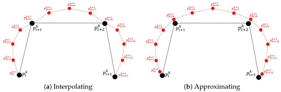
Figure 1. The configuration of new points for the interpolating and approximating QSS for curves; the solid lines are the control polygon, and the dotted lines are the refined polygon.

Since the combination is affine it holds

$$\sum _{m=0}^{N-1}{a}_{\alpha ,m}=1,\alpha =0,1,2,3.$$

(2)

The adjustment of the coefficients for the computation of error bound and subdivision depth is

$$\begin{array}{c}\hfill \left\{\begin{array}{c}{e}_{\beta ,m}={\displaystyle \sum _{l=0}^m}(a_{\beta ,l}-a_{\beta +1,l}),\beta =0,1,2,\hfill \\ e_{3,m}=a_{0,m}-{\displaystyle \sum _{\beta =0}^2}{e}_{\beta ,m},\hfill \end{array}\right.\end{array}$$

(3)

along with the strict condition (See [15])

$$\sum _{m=0}^{N-1}\left|e_{\beta ,m}\right|<1,\beta =0,1,2,3.$$

(4)

Here, we introduce some new notations, for $m=0,1,\dots ,N-1$, as follows

$$\begin{array}{c}\hfill \left\{\begin{array}{c}{b}_{4m}=e_{0,m},\hfill \\ b_{4m+1}=e_{1,m},\hfill \\ b_{4m+2}=e_{2,m},\hfill \\ b_{4m+3}=e_{3,m}.\hfill \end{array}\right.\end{array}$$

(5)

Furthermore, to be more specific, update the track defined in [20] for the computation of error bounds and subdivision depth. Let, at the kth level of resolution, the vector $v_i=p_i^k$ represents the approximation coefficients. Then the approximation coefficients of two consecutive stages k and $k+1$ in the reconstruction process of QSS is defined as

$$p_i^{k+1}=\sum _{n\in \mathbb{N}}{b}_{i-4n}{p}_n^k={(p^{k;0}🟉b)}_i,$$

(6)

where $v_i^0=p_i^{k;0}$ shows the $k^{th}$ resolution level and ${}^{\prime }🟉{}^{\prime }$ shows the convolution product. If $p^{k;0}=\{p^{k;0};n\ge 0\}$ and $b=\{b_n;n\ge 0\}$ are finite vectors with length ${\gamma }_1$ and ${\gamma }_2$ respectively then

$${(p^{k;0}🟉b)}_j=\sum _{n=max\{j-({\gamma }_2-1),0\}}^{min\{j,{\gamma }_1-1\}}{p}_n^{k;0}{b}_{j-4n},j=0,1,\dots ,{\gamma }_1+{\gamma }_1-2.$$

(7)

Now we move forward and present some results of successive convolutions for one-dimensional array of vectors based on QSS.

Lemma 1.

Let $p={\left\{p_n\right\}}_{n\ge 0}$ and $b={\left\{b_n\right\}}_{n=0}^{4N-1}$ with $b_n=0$ for $n\ge 4N$ be finite one-dimensional arrays of vectors. Then for QSS, the one-dimensional $l_0$ convolution of these vectors satisfies the following inequality

$$\begin{array}{c}\hfill \parallel ({(\dots {(({(p^{\left(0\right)}🟉b)}^{\left(0\right)})🟉b)}^{\left(0\right)}🟉\dots 🟉b)}^{\left(0\right)}🟉b){\parallel }_{\infty }\le {\parallel p\parallel }_{\infty }\underset{j}{max}\left\{\sum _{m=0}^{\lfloor j/4^{l_0}\rfloor }\left|A_{m,j}^{l_0}\right|\right\},\end{array}$$

(8)

where

$$\begin{array}{c}\hfill \left\{\begin{array}{c}{A}_{m,j}^1=b_{j-4m},\hfill \\ A_{m,j}^{l_0}={\displaystyle \sum _{p=4m}^{\lfloor j/4^{l_0-1}\rfloor }}{A}_{m,p}^1{A}_{p,j}^{l_0-1},l_0\ge 2,\hfill \end{array}\right.\end{array}$$

(9)

and

$$\begin{array}{ccc}\hfill j\in \sum (l_0,N)& =& \{\mathsf{\Omega }(l_0,N)-4^{l_0}+1,\mathsf{\Omega }(l_0,N)-4^{l_0}+2,\dots ,\mathsf{\Omega }(l_0,N)\},\hfill \end{array}$$

(10)

$$\begin{array}{ccc}\hfill \mathsf{\Omega }(l_0,N)& =& (4^{l_0}-3)(4N-1).\hfill \end{array}$$

(11)

Proof. 

See Appendix A.1. □

Lemma 2.

For QSS, the term $A_{m,j}^{l_0}$ defined by (9) satisfies the following equality

$$A_{m-1,j-4^{l_0}}^{l_0}=A_{m,j}^{l_0}=A_{m+1,j+4^{l_0}}^{l_0}.$$

(12)

Proof. 

See Appendix A.2. □

Corollary 1.

The term $\underset{j}{max}\left\{{\displaystyle \sum _{m=0}^{\lfloor j/4^{l_0}\rfloor }}\left|A_{m,j}^{l_0}\right|\right\}$ involved in the inequality (8) satisfies the following equality

$$B_{l_0}=\underset{j}{max}\left\{\sum _{m=0}^{\lfloor j/4^{l_0}\rfloor }\left|A_{m,j}^{l_0}\right|\right\}=\underset{j\in \sum (l_0,N)}{max}\left\{\sum _{m=0}^{\lfloor j/4^{l_0}\rfloor }\left|A_{m,j}^{l_0}\right|\right\}.$$

(13)

Proof. 

See Appendix A.3. □

Now, we present the inequalities to compute the error bound and subdivision depth for the curve models produced by QSS.

Theorem 1.

If $P^0=\{p_i^0,i\in \mathbb{Z}\}$ is the initial polygon and $P^k=\{p_i^k,i\in \mathbb{Z}\}$ is the polygon obtained by QSS at $k^{th}$ subdivision level. Then the error bound between two successive levels is

$$\begin{array}{c}\hfill \parallel P^{k+1}-P^k{\parallel }_{\infty }\le \psi \chi {\left(B_{l_0}\right)}^k,\end{array}$$

(14)

where $B_{l_0},l_0\ge 1$ defined in (13),

$$\chi =\underset{i}{max}∥p_{i+1}^0-p_i^0∥,\psi =\underset{\alpha }{max}\left(\left|\sum _{m=0}^{N-2}{\tilde{a}}_{\alpha ,m}\right|,\alpha =0,1,2,3\right),$$

and

$$\begin{array}{c}\hfill \left\{\begin{array}{c}{\tilde{a}}_{\alpha ,0}={\displaystyle \sum _{l=1}^{N-1}}{a}_{\alpha ,l}-\frac{\alpha }{4},\hfill \\ \\ {\tilde{a}}_{\alpha ,m}={\displaystyle \sum _{l=m+1}^{N-1}}{a}_{\alpha ,l},m\ge 1,\alpha =0,1,2,3.\hfill \end{array}\right.\end{array}$$

We omit the proof since it is similar to the one given in [15].

Theorem 2.

If we assume the same conditions as in the Theorem 1 with the limiting curve model $P^{\infty }$ then the error bounds ${\nabla }^k$ between the limiting curve model and its $k^{th}$ level polygon satisfies the inequality

$${\nabla }^k={\parallel P^{\infty }-P^k\parallel }_{\infty }\le \psi \chi \left(\frac{{\left(B_{l_0}\right)}^k}{1-B_{l_0}}\right),$$

(15)

where $l_0\ge 1$, such that $B_{l_0}<1$.

By looking at the proof of Theorem 2.1 of [15] one may lead to prove of Theorem 2.

Given a user tolerable error $ϵ>0$, the subdivision depth of limiting model $P^{\infty }$ generated by QSS concerning for $ϵ$ is a positive integer k such that the error bound ${\nabla }^k\le ϵ$. In the following theorem, we compute the subdivision depth.

Theorem 3.

If we assume the same conditions as in the Theorem 2 with the user tolerable error $ϵ>0$ and

$$k\ge {log}_{B_{l_0}}\left(\frac{ϵ(1-B_{l_0})}{\psi \chi }\right),$$

(16)

then ${\nabla }^k\le ϵ$.

3. The Error Bounds and Subdivision Depth for Surface Models

In this work, we first generalize the results presented in Lemma 1 to Lemma 2 and Corollary 1 for two-dimensional arrays then we generalize the inequalities of Theorems 1–3 to compute the error bound and subdivision depth of the limiting tensor product surface models generated by QSS.

For this, let ${\mathbf{P}}^k=\{p_{i,j}^k;i,j\in \mathbb{Z}\}$ be the polygon made by the sequence of points in ${\mathbf{R}}^{\aleph }$, where $\aleph \ge 2$ and the polygon ${\mathbf{P}}^{k+1}=\{p_{i,j}^{k+1};i,j\in \mathbb{Z}\}$ be obtained by the tensor product of the scheme (1). The graphical representation of the points at kth and $(k+1)$th levels is shown in Figure 2 whereas the mathematical form of tensor product QSS is described as

$$p_{4i+\alpha ,4j+\gamma }^{k+1}=\sum _{r=0}^{N-1}\sum _{s=0}^{N-1}{a}_{\alpha ,r}{a}_{\gamma ,s}{p}_{i+r,m+s}^k,\alpha ,\gamma =0,1,2,3,$$

(17)

where $a_{\alpha ,r}$ and $a_{\gamma ,s}$ satisfies (2).

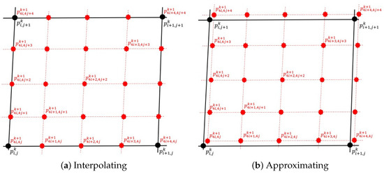
Figure 2. The configuration of new points for the interpolating and approximating QSS for the surface. The solid lines show one face of coarse polygon while the dotted lines show the faces of the refined polygon.

Here we introduce new notations $c={\left\{c_n\right\}}_{n\in N}$, $d={\left\{d_n\right\}}_{n\in N}$ for $r,s=0,1,\dots ,N-1,$ such that

$$\begin{array}{c}\hfill \left\{\begin{array}{c}{c}_{4r}=a_{0,N-r-1},\hfill \\ c_{4r+1}=a_{1,N-r-1},\hfill \\ c_{4r+2}=a_{2,N-r-1},\hfill \\ c_{4r+3}=a_{3,N-r-1}r=0,∆,N-1.\hfill \\ d_{4s}=b_{0,N-s-1}\hfill \\ d_{4s+1}=b_{1,N-s-1}\hfill \\ d_{4s+2}=b_{2,N-s-1}\hfill \\ d_{4s+3}=b_{3,N-s-1}s=0,∆,N-1.\hfill \end{array}\right.\end{array}$$

(18)

Since the extension of some of the results from one dimension array of vectors to two-dimensional array is straight forward (See [15]), therefore we skip the trivial explanations and directly come to the following result.

Lemma 3.

Let $p_{i,j}$ be a finite two-dimensional array of vectors and $d={\left\{d_n\right\}}_{n=0}^{4N-1}$, $c={\left\{c_n\right\}}_{n=0}^{4N-1}$ with $d_n=c_n=0$ for $n\ge 4N$ are one-dimensional arrays of vectors. Then, for QSS, the two-dimensional $l_0$ convolution satisfies the following inequality

$$\begin{array}{c}\hfill \underset{i,j}{max}|p_{i,j}^{l_0}|\le C_{l_0}{D}_{l_0}\underset{m,n}{max}\left|p_{m,n}^0\right|.\end{array}$$

(19)

Here

$$C_{l_0}=\underset{i}{max}\left\{\sum _{m=0}^{\lfloor i/4^{l_0}\rfloor }\left|A_{m,i}^{l_0,c}\right|\right\}$$

(20)

and

$$D_{l_0}=\underset{j}{max}\left\{\sum _{n=0}^{\lfloor j/4^{l_0}\rfloor }\left|A_{n,j}^{l_0,d}\right|\right\}.$$

(21)

where

$$\begin{array}{c}\hfill \left\{\begin{array}{c}{A}_{m,i}^{1,c}=c_{i-4m},\hfill \\ A_{m,i}^{l_0,c}={\displaystyle \sum _{p=4m}^{\lfloor i/4^{l_0-1}\rfloor }}{A}_{m,p}^{1,c}{A}_{p,i}^{l_0-1,c},\hfill \\ A_{n,j}^{1,d}=d_{j-4n},\hfill \\ A_{n,j}^{l_0,d}={\displaystyle \sum _{q=4n}^{\lfloor j/4^{l_0-1}\rfloor }}{A}_{n,q}^{1,d}{A}_{q,j}^{l_0-1,d},l_0\ge 2,\hfill \end{array}\right.\end{array}$$

Proof. 

See Appendix A.4. □

Now, we present the inequalities to compute the error bound and subdivision depth for the surface models produced by QSS. By using a similar approach of [15], one can easily prove the Theorems 4 and 5.

Theorem 4.

If ${\mathit{P}}^0=\{p_{i,j}^0,i\in \mathbb{Z}\}$ is the initial polygon and ${\mathit{P}}^k=\{p_{i,j}^k,i\in \mathbb{Z}\}$ is the polygon obtained by (17). Then the error bound between two successive levels is

$$\begin{array}{c}\hfill \parallel {\mathit{P}}^{k+1}-{\mathit{P}}^k{\parallel }_{\infty }\le \nu {\left(C_{l_0}{D}_{l_0}\right)}^k.\end{array}$$

(22)

Here $C_{l_0},D_{l_0}$ for $l_0\ge 1$ is defined in (20) and (21) and $\nu =\underset{\alpha ,\beta }{max}\left\{{\sum }_{t=1}^3\left({\chi }_t\right)\left({\psi }_{\alpha ,\beta }^t\right),\alpha ,\beta =0,1,2,3\right\},$ where ${\chi }_t$ and ${\psi }_{\alpha ,\beta }^t$ for $\alpha ,\beta =0,1,2,3$ are defined in [15].

Theorem 5.

If we assume the same conditions as in the Theorem 4 with the limiting surface model ${\mathit{P}}^{\infty }$ then the error bound ${\nabla }^k$ between the limiting surface model and its kth level polygon is defined by the inequality

$${\nabla }^k={\parallel {\mathit{P}}^{\infty }-{\mathit{P}}^k\parallel }_{\infty }\le \nu \left(\frac{{\left(C_{l_0}{D}_{l_0}\right)}^k}{1-C_{l_0}{D}_{l_0}}\right),$$

(23)

where $l_0\ge 1$, such that $C_{l_0}{D}_{l_0}<1$.

In the following theorem, we present the subdivision depth for the surface model.

Theorem 6.

If we assume the same conditions as in the Theorem 5 with the user tolerable error $ϵ>0$ and if

$$k\ge {log}_{\left(C_{l_0}{D}_{l_0}\right)}\left(\frac{ϵ(1-C_{l_0}{D}_{l_0})}{\nu }\right),$$

(24)

then ${\nabla }^k\le ϵ$.

4. Numerical Applications for Curve Models

In this section, we demonstrate the performance of our inequalities to compute error bound and subdivision depth of the curve models. First, we compute $B_{l_0}$ defined in (13) at different values of $l_0$.

Example 1.

If the curve model is produced by a 3-point approximating QSS [2] with coefficients $a_{0,0}=\frac{49}{128}$, $a_{0,1}=\frac{39}{64}$, $a_{0,2}=\frac{1}{128}$, $a_{1,0}=\frac{25}{128}$, $a_{1,1}=\frac{47}{64}$, $a_{1,2}=\frac{9}{128}$, $a_{2,0}=\frac{9}{128}$, $a_{2,1}=\frac{47}{64}$, $a_{2,2}=\frac{25}{128}$, $a_{3,0}=\frac{1}{128}$, $a_{3,1}=\frac{39}{64}$, $a_{3,2}=\frac{49}{128}$. Then for $N=3$, we have

$$B_{l_0}=\underset{j\in \sum (l_0,3)}{max}\left\{\sum _{m=0}^{\lfloor j/4^{l_0}\rfloor }\left|A_{m,j}^{l_0}\right|\right\}.$$

For $l_0=1$, we get

$$\begin{array}{ccc}\hfill B_1& =& \underset{j\in \sum (1,3)}{max}\left\{\sum _{m=0}^{\lfloor j/4\rfloor }\left|A_{m,j}^1\right|\right\}=\underset{j\in \{8,9,10,11\}}{max}\left\{\sum _{m=0}^{\lfloor j/4\rfloor }\left|b_{j-4m}\right|\right\}.\hfill \end{array}$$

Using (5) and Lemma 1, we have $b={\left\{b_n\right\}}_{n=0}^{11}$ with $b_n=0$ for $n\ge 12$. Hence

$$\left\{b_0,b_1,b_2,b_3,b_4,b_5,b_6,b_7,b_8,b_9,b_{10},b_{11}\right\}=\left\{\frac{24}{128},\frac{16}{128},\frac{8}{128},\frac{1}{128},\frac{8}{128},\frac{16}{128},\frac{24}{128},\frac{30}{128},0,0,0,\frac{1}{128}\right\}.$$

(25)

Now consider

$$\begin{array}{ccc}\hfill B_1& =& max\left\{\sum _{m=0}^{\lfloor 8/4\rfloor }|b_{8-4m}|,\sum _{m=0}^{\lfloor 9/4\rfloor }|b_{9-4m}|,\sum _{m=0}^{\lfloor 10/4\rfloor }|b_{10-4m}|,\sum _{m=0}^{\lfloor 11/4\rfloor }|b_{11-4m}|\right\}.\hfill \end{array}$$

This implies

$$\begin{array}{ccc}\hfill B_1& =& max\left\{|b_8|+|b_4|+|b_0|,|b_9|+|b_5|+|b_1|,|b_{10}|+|b_6|+|b_2|,|b_{11}|+|b_7|+|b_3|\right\}\hfill \\ & =& max\left\{0+\left|\frac{8}{128}\right|+\left|\frac{24}{128}\right|,0+\left|\frac{16}{128}\right|+\left|\frac{16}{128}\right|,0+\left|\frac{24}{128}\right|+\left|\frac{8}{128}\right|,\left|\frac{1}{128}\right|+\left|\frac{30}{128}\right|+\left|\frac{1}{128}\right|\right\}\hfill \\ & =& \frac{1}{4}.\hfill \end{array}$$

For $l_0=2$, we get

$$\begin{array}{ccc}\hfill B_2& =& \underset{j\in \sum (2,3)}{max}\left\{\sum _{m=0}^{\lfloor j/4^2\rfloor }\left|A_{m,j}^2\right|\right\}=\underset{j\in \{128,129,\dots ,143\}}{max}\left\{\sum _{m=0}^{\lfloor j/16\rfloor }\left|A_{m,j}^2\right|\right\}\hfill \\ & =& \underset{j\in \{128,129,\dots ,143\}}{max}\left\{\sum _{m=0}^{\lfloor j/16\rfloor }\left|\sum _{n=4m}^{\lfloor j/4\rfloor }{A}_{m,n}^1{A}_{n,j}^1\right|\right\}.\hfill \end{array}$$

This implies

$$\begin{array}{ccc}\hfill B_2& =& max\left\{\sum _{m=0}^{\lfloor 128/16\rfloor }\right|\sum _{n=4m}^{\lfloor 128/4\rfloor }{A}_{m,n}^1{A}_{n,128}^1|,\sum _{m=0}^{\lfloor 129/16\rfloor }|\sum _{n=4m}^{\lfloor 129/4\rfloor }{A}_{m,n}^1{A}_{n,129}^1|,\sum _{m=0}^{\lfloor 130/16\rfloor }|\sum _{n=4m}^{\lfloor 130/4\rfloor }{A}_{m,n}^1{A}_{n,130}^1|,\hfill \\ & & \sum _{m=0}^{\lfloor 131/16\rfloor }\left|\sum _{n=4m}^{\lfloor 131/4\rfloor }{A}_{m,n}^1{A}_{n,131}^1\right|,\sum _{m=0}^{\lfloor 132/16\rfloor }\left|\sum _{n=4m}^{\lfloor 132/4\rfloor }{A}_{m,n}^1{A}_{n,132}^1\right|,\sum _{m=0}^{\lfloor 133/16\rfloor }\left|\sum _{n=4m}^{\lfloor 133/4\rfloor }{A}_{m,n}^1{A}_{n,133}^1\right|,\hfill \\ & & \sum _{m=0}^{\lfloor 134/16\rfloor }\left|\sum _{n=4m}^{\lfloor 134/4\rfloor }{A}_{m,n}^1{A}_{n,134}^1\right|,\sum _{m=0}^{\lfloor 135/16\rfloor }\left|\sum _{n=4m}^{\lfloor 135/4\rfloor }{A}_{m,n}^1{A}_{n,135}^1\right|,\sum _{m=0}^{\lfloor 136/16\rfloor }\left|\sum _{n=4m}^{\lfloor 136/4\rfloor }{A}_{m,n}^1{A}_{n,136}^1\right|,\hfill \\ & & \sum _{m=0}^{\lfloor 137/16\rfloor }\left|\sum _{n=4m}^{\lfloor 137/4\rfloor }{A}_{m,n}^1{A}_{n,137}^1\right|,\sum _{m=0}^{\lfloor 138/16\rfloor }\left|\sum _{n=4m}^{\lfloor 138/4\rfloor }{A}_{m,n}^1{A}_{n,138}^1\right|,\sum _{m=0}^{\lfloor 139/16\rfloor }\left|\sum _{n=4m}^{\lfloor 139/4\rfloor }{A}_{m,n}^1{A}_{n,139}^1\right|,\hfill \\ & & \sum _{m=0}^{\lfloor 140/16\rfloor }\left|\sum _{n=4m}^{\lfloor 140/4\rfloor }{A}_{m,n}^1{A}_{n,140}^1\right|,\sum _{m=0}^{\lfloor 141/16\rfloor }\left|\sum _{n=4m}^{\lfloor 141/4\rfloor }{A}_{m,n}^1{A}_{n,141}^1\right|,\sum _{m=0}^{\lfloor 142/16\rfloor }\left|\sum _{n=4m}^{\lfloor 142/4\rfloor }{A}_{m,n}^1{A}_{n,142}^1\right|,\hfill \\ & & \sum _{m=0}^{\lfloor 143/16\rfloor }\left|\sum _{n=4m}^{\lfloor 143/4\rfloor }{A}_{m,n}^1{A}_{n,143}^1\right|\}.\hfill \end{array}$$

This further implies

$$\begin{array}{ccc}\hfill B_2& =& max\left\{{\lambda }_1,{\lambda }_2,{\lambda }_3,{\lambda }_4,{\lambda }_5,{\lambda }_6,{\lambda }_7,{\lambda }_8,{\lambda }_9,{\lambda }_{10},{\lambda }_{11},{\lambda }_{12},{\lambda }_{13},{\lambda }_{14},{\lambda }_{15},{\lambda }_{16}\right\}.\hfill \end{array}$$

Since $b_i=0$, for all $i>11$, therefore we have

$$\begin{array}{ccc}\hfill {\lambda }_1& =& |b_4{b}_{11}+b_8{b}_{10}|+|b_0{b}_8+b_4{b}_7+b_6{b}_8|+|b_0{b}_4+b_2{b}_8+b_3{b}_4|+|b_0{|}^2,\hfill \end{array}$$

$$\begin{array}{ccc}\hfill {\lambda }_2& =& |b_5{b}_{11}+b_9{b}_{10}|+|b_1{b}_8+b_5{b}_7+b_6{b}_9|+|b_1{b}_4+b_2{b}_9+b_3{b}_5|+\left|b_0{b}_1\right|,\hfill \end{array}$$

$$\begin{array}{ccc}\hfill {\lambda }_3& =& |b_6{b}_{11}+b_{10}^2|+|b_2{b}_8+b_6{b}_7+b_6{b}_{10}|+|b_2{b}_4+b_2{b}_{10}+b_3{b}_6|+|b_0+b_2|,\hfill \end{array}$$

$$\begin{array}{ccc}\hfill {\lambda }_4& =& |b_7{b}_{11}+b_{10}{b}_{11}|+|b_3{b}_8+b_6{b}_{11}+b_7^2|+|b_2{b}_{11}+b_3{b}_4+b_3{b}_7|+\left|b_0{b}_3\right|,\hfill \end{array}$$

$$\begin{array}{ccc}\hfill {\lambda }_5& =& \left|b_{11}{b}_8\right|+|b_0{b}_9+b_4{b}_8+b_7{b}_8|+|b_0{b}_5+b_3{b}_8+b_4^2|+|b_0{b}_1+b_0{b}_4|,\hfill \end{array}$$

$$\begin{array}{ccc}\hfill {\lambda }_6& =& \left|b_{11}{b}_9\right|+|b_1{b}_9+b_5{b}_8+b_7{b}_9|+|b_1{b}_5+b_3{b}_9+b_4{b}_5|+|b_0{b}_5+b_1^2|,\hfill \end{array}$$

$$\begin{array}{ccc}\hfill {\lambda }_7& =& \left|b_{10}{b}_{11}\right|+|b_2{b}_9+b_6{b}_8+b_7{b}_{10}|+|b_2{b}_5+b_3{b}_{10}+b_4{b}_6|+|b_0{b}_6+b_1{b}_2|,\hfill \end{array}$$

$$\begin{array}{ccc}\hfill {\lambda }_8& =& \left|b_{11}^2\right|+|b_3{b}_9+b_7{b}_8+b_7{b}_{11}|+|b_3{b}_5+b_3{b}_{11}+b_4{b}_7|+|b_0{b}_7+b_1{b}_3|,\hfill \end{array}$$

$$\begin{array}{ccc}\hfill {\lambda }_9& =& |b_0{b}_{10}+b_4{b}_9+b_8^2|+|b_0{b}_6+b_4{b}_5+b_4{b}_8|+|b_0{b}_2+b_0{b}_8+b_1{b}_4|,\hfill \end{array}$$

$$\begin{array}{ccc}\hfill {\lambda }_{10}& =& |b_1{b}_{10}+b_5{b}_9+b_8{b}_9|+|b_1{b}_6+b_4{b}_9+b_5^2|+|b_0{b}_9+b_1{b}_2+b_1{b}_5|,\hfill \end{array}$$

$$\begin{array}{ccc}\hfill {\lambda }_{11}& =& |b_2{b}_{10}+b_6{b}_9+b_8{b}_{10}|+|b_2{b}_6+b_4{b}_{10}+b_5{b}_6|+|b_0{b}_{10}+b_1{b}_6+b_2^2|,\hfill \end{array}$$

$$\begin{array}{ccc}\hfill {\lambda }_{12}& =& |b_3{b}_{10}+b_7{b}_9+b_8{b}_{11}|+|b_3{b}_6+b_4{b}_{11}+b_5{b}_7|+|b_0{b}_{11}+b_1{b}_7+b_2{b}_3|,\hfill \end{array}$$

$$\begin{array}{ccc}\hfill {\lambda }_{13}& =& |b_0{b}_{11}+b_4{b}_{10}+b_8{b}_9|+|b_0{b}_7+b_4{b}_6+b_5{b}_8|+|b_0{b}_3+b_1{b}_8+b_2{b}_4|,\hfill \end{array}$$

$$\begin{array}{ccc}\hfill {\lambda }_{14}& =& |b_1{b}_{11}+b_5{b}_{10}+b_9^2|+|b_1{b}_7+b_5{b}_6+b_5{b}_9|+|b_1{b}_3+b_1{b}_9+b_2{b}_5|,\hfill \end{array}$$

$$\begin{array}{ccc}\hfill {\lambda }_{15}& =& |b_2{b}_{11}+b_6{b}_{10}+b_9{b}_{10}|+|b_2{b}_7+b_5{b}_{10}+b_6^2|+|b_1{b}_{10}+b_2{b}_3+b_2{b}_6|,\hfill \end{array}$$

$$\begin{array}{ccc}\hfill {\lambda }_{16}& =& |b_3{b}_{11}+b_7{b}_{10}+b_9{b}_{11}|+|b_3{b}_7+b_5{b}_{11}+b_6{b}_7|+|b_1{b}_{11}+b_2{b}_7+b_3^2|\}.\hfill \end{array}$$

Now using (25), we acquire

$$\begin{array}{ccc}\hfill B_2& =& max\left\{\right|b_4{b}_{11}+b_8{b}_{10}|+|b_0{b}_8+b_4{b}_7+b_6{b}_8|+|b_0{b}_4+b_2{b}_8+b_3{b}_4|+|b_0{|}^2,|b_5{b}_{11}+b_9{b}_{10}|\hfill \\ & & +|b_1{b}_8+b_5{b}_7+b_6{b}_9|+|b_1{b}_4+b_2{b}_9+b_3{b}_5|+|b_0{b}_1|,|b_6{b}_{11}+b_{10}^2|+|b_2{b}_8+b_6{b}_7+b_6{b}_{10}|\hfill \\ & & +|b_2{b}_4+b_2{b}_{10}+b_3{b}_6|+|b_0+b_2|,|b_7{b}_{11}+b_{10}{b}_{11}|+|b_3{b}_8+b_6{b}_{11}+b_7^2|+|b_2{b}_{11}+b_3{b}_4\hfill \\ & & +b_3{b}_7|+|b_0{b}_3|,0+0+|b_0{b}_5+b_3{b}_8+b_4^2|+|b_0{b}_1+b_0{b}_4|,0+0+|b_1{b}_5+b_3{b}_9+b_4{b}_5|\hfill \\ & & +|b_0{b}_5+b_1^2|,0+0+|b_2{b}_5+b_3{b}_{10}+b_4{b}_6|+|b_0{b}_6+b_1{b}_2|,|b_{11}^2|+|b_3{b}_9+b_7{b}_8+b_7{b}_{11}|\hfill \\ & & +|b_3{b}_5+b_3{b}_{11}+b_4{b}_7|+|b_0{b}_7+b_1{b}_3|,0+|b_0{b}_6+b_4{b}_5+b_4{b}_8|+|b_0{b}_2+b_0{b}_8+b_1{b}_4|,\hfill \\ & & 0+|b_1{b}_6+b_4{b}_9+b_5^2|+|b_0{b}_9+b_1{b}_2+b_1{b}_5|,0+|b_2{b}_6+b_4{b}_{10}+b_5{b}_6|+|b_0{b}_{10}+b_1{b}_6+b_2^2|\hfill \\ & & ,0+|b_3{b}_6+b_4{b}_{11}+b_5{b}_7|+|b_0{b}_{11}+b_1{b}_7+b_2{b}_3|,|b_0{b}_{11}+b_4{b}_{10}+b_8{b}_9|+|b_0{b}_7+b_4{b}_6\hfill \\ & & +b_5{b}_8|+|b_0{b}_3+b_1{b}_8+b_2{b}_4|,|b_1{b}_{11}+b_5{b}_{10}+b_9^2|+|b_1{b}_7+b_5{b}_6+b_5{b}_9|+|b_1{b}_3+b_1{b}_9\hfill \\ & & +b_2{b}_5|,|b_2{b}_{11}+b_6{b}_{10}+b_9{b}_{10}|+|b_2{b}_7+b_5{b}_{10}+b_6^2|+|b_1{b}_{10}+b_2{b}_3+b_2{b}_6|,|b_3{b}_{11}+b_7{b}_{10}\hfill \\ & & +b_9{b}_{11}|+|b_3{b}_7+b_5{b}_{11}+b_6{b}_7|+|b_1{b}_{11}+b_2{b}_7+b_3^2\left|\right\}.\hfill \end{array}$$

This implies that

$$\begin{array}{ccc}\hfill B_2& =& max\left\{\frac{1}{16},\frac{1}{16},\frac{1}{16},\frac{1}{16},\frac{1}{16},\frac{1}{16},\frac{1}{16},\frac{1}{16},\frac{1}{16},\frac{1}{16},\frac{1}{16},\frac{1}{16},\frac{1}{16},\frac{1}{16},\frac{1}{16},\frac{1}{16}\right\}=\frac{1}{16}.\hfill \end{array}$$

Similarly, we can compute the values of $B_{l_0}$ for $l_0\ge 3$. For convenience, we have computed the values up to $l_0=4$, which are shown in Table 1. The subdivision depth k by Theorem 3 at different values of $B_{l_0}$ are given in Table 2.

Table 1. Values of $B_{l_0}$ for $l_0=1,2,3,4.$

Scheme/${\mathit{B}}_{{\mathit{l}}_0}$	${\mathit{B}}_1={\mathit{\delta }}_1$ [15]	${\mathit{B}}_2$	${\mathit{B}}_3$	${\mathit{B}}_4$
3-point approximating curve [2]	0.250000	0.062500	0.015625	0.003906
4-point approximating curve [1]	0.250000	0.062500	0.015625	0.003906
4-point interpolating curve [4]	0.328125	0.105957	0.034286	0.011092

Table 2. Depth of a 3-point approximating QSS curve model.

${\mathit{B}}_{{\mathit{l}}_0}$/$\mathit{ϵ}$	$2.45\times {10}^{-3}$	$9.57\times {10}^{-7}$	$3.74\times {10}^{-9}$	$1.46\times {10}^{-11}$	$5.7\times {10}^{-14}$	$2.23\times {10}^{-16}$	$8.7\times {10}^{-19}$
$B_1={\delta }_1$ [15]	4	8	12	16	20	24	28
$B_2$	2	4	6	8	10	12	14
$B_3$	1	3	4	5	7	8	9
$B_4$	1	2	3	4	5	6	7

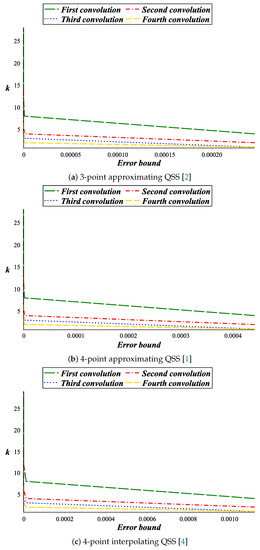
In this work, $B_{l_0}$ for $l_0=1$ is equal to ${\delta }_1$ defined in [15]. If ${\delta }_1>1$, then the error bound of QSS cannot be computed. However, in the proposed approach, if we increase the value of $l_0$, the values of $B_{l_0}$ decreases until $B_{l_0}$ becomes less than one. The main advantage of this approach also to compute error bounds of those QSS, whose ${\delta }_1$ is greater or equal to one. As in Table 2, twenty-eight iterations are needed to achieve a given error tolerance $8.7\times {10}^{-19}$ by technique given in [15], but by our technique, it needs only seven iterations corresponding to $B_4$. The graphical comparison between the results at first and fourth convolutions are demonstrated in Figure 3a.

Figure 3. The comparison between various convolutions for curve case.

Example 2.

The subdivision depth of the curve model produced by a 4-point approximating QSS [1] are given in Table 3. The graphical view of these depths is shown in Figure 3b.

Table 3. Depth of a 4-point approximating QSS curve model.

${\mathit{B}}_{{\mathit{l}}_0}$/$\mathit{ϵ}$	$4.41\times {10}^{-4}$	$1.72\times {10}^{-6}$	$6.73\times {10}^{-9}$	$2.63\times {10}^{-11}$	$1.03\times {10}^{-13}$	$4.01\times {10}^{-16}$	$1.57\times {10}^{-18}$
$B_1={\delta }_1$ [15]	4	8	12	16	20	24	28
$B_2$	2	4	6	8	10	12	14
$B_3$	1	3	4	5	7	8	9
$B_4$	1	2	3	4	5	6	7

Example 3.

The subdivision depths of the curve model produced by a 4-point interpolating QSS [4] for $B_{l_0},l_0\ge 1$ (see Table 1) are shown in Table 4. From Table 4, we can observe that the number of iterations k (subdivision depth) decreases with the increase of $l_0$ (order of convolution) to obtain a user given error tolerance. This is the main reason for the reduction of computational cost as compared to the technique given by [15]. The graphical analysis can be seen in Figure 3c.

Table 4. Depth of a 4-point interpolating QSS curve model.

${\mathit{B}}_{{\mathit{l}}_0}$/$\mathit{ϵ}$	$1.12\times {10}^{-3}$	$1.24\times {10}^{-5}$	$1.38\times {10}^{-7}$	$1.53\times {10}^{-9}$	$1.7\times {10}^{-11}$	$1.88\times {10}^{-13}$	$2.09\times {10}^{-15}$
$B_1={\delta }_1$ [15]	4	8	12	16	21	25	29
$B_2$	2	4	6	8	10	12	14
$B_3$	1	3	4	5	7	8	9
$B_4$	1	2	3	4	5	6	7

5. Numerical Applications for Surface Models

Now we demonstrate the performance of our results to compute error bound and subdivision depth of the surface models. First, we compute the term $C_{l_0}{D}_{l_0}$ for $l_0\ge 1$ by using (20) and (21). These are shown in Table 5. We see that the values of $C_{l_0}{D}_{l_0}$ decrease with the increase of $l_0$. This is the advantage of our approach.

Table 5. The values of $C_{l_0}{D}_{l_0}$ for $l_0=1,2,3,4$.

Scheme/${\mathit{C}}_{{\mathit{l}}_0}{\mathit{D}}_{{\mathit{l}}_0}$	${\mathit{C}}_1{\mathit{D}}_1={\mathit{\delta }}_2$ [15]	${\mathit{C}}_2{\mathit{D}}_2$	${\mathit{C}}_3{\mathit{D}}_3$	${\mathit{C}}_4{\mathit{D}}_4$
3-point QSS for surface [2]	0.250000	0.062500	0.015625	0.003906
4-point QSS for surface [1]	0.264140	0.065694	0.016672	0.004209
4-point QSS for surface [4]	0.389648	0.140310	0.049504	0.017476

Example 4.

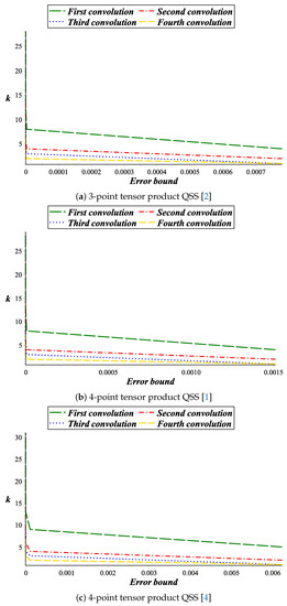
The subdivision depths of the surface model produced by the tensor product of a 3-point approximating QSS [2] are given in Table 6. The values are computed by using the Theorem 6. The graphical representation is shown in Figure 4a.

Table 6. Depth of the 3-point approximating QSS surface model.

${\mathit{C}}_{{\mathit{l}}_0}{\mathit{D}}_{{\mathit{l}}_0}$/$\mathit{ϵ}$	$7.8\times {10}^{-4}$	$3.05\times {10}^{-6}$	$1.19\times {10}^{-8}$	$4.65\times {10}^{-11}$	$1.82\times {10}^{-13}$	$7.1\times {10}^{-16}$	$2.77\times {10}^{-18}$
$C_1{D}_1=\delta 2$ [15]	4	8	12	16	20	24	28
$C_2{D}_2$	2	4	6	8	10	12	14
$C_3{D}_3$	1	3	4	5	7	8	9
$C_4{D}_4$	1	2	3	4	5	6	7

Figure 4. The comparison between different convolutions for the surface case.

Example 5.

The subdivision depths of the surface model produced by the tensor product of a 4-point approximating QSS [1] are shown in Table 7. Also, these depths are graphically shown in Figure 4b.

Table 7. Depth of the 4-point approximating QSS surface model.

${\mathit{C}}_{{\mathit{l}}_0}{\mathit{D}}_{{\mathit{l}}_0}$/$\mathit{ϵ}$	$1.51\times {10}^{-3}$	$6.36\times {10}^{-6}$	$2.68\times {10}^{-8}$	$1.13\times {10}^{-10}$	$4.74\times {10}^{-13}$	$1.99\times {10}^{-15}$	$8.4\times {10}^{-18}$
$C_1{D}_1={\delta }_2$ [15]	4	8	13	17	21	25	29
$C_2{D}_2$	2	4	6	8	10	12	14
$C_3{D}_3$	1	3	4	5	7	8	9
$C_4{D}_4$	1	2	3	4	5	6	7

Example 6.

The subdivision depth of a 4-point interpolating QSS surface model [4] corresponding to $C_{l_0}{D}_{l_0},l_0\ge 1$ (see Table 5) is shown in Table 8. The graphical view of the first and fourth convolutions is given in Figure 4c.

Table 8. Depth of a 4-point interpolating QSS surface model.

${\mathit{C}}_{{\mathit{l}}_0}{\mathit{D}}_{{\mathit{l}}_0}$/$\mathit{ϵ}$	$6.22\times {10}^{-3}$	$1.09\times {10}^{-4}$	$1.9\times {10}^{-6}$	$3.32\times {10}^{-8}$	$5.81\times {10}^{-10}$	$1.01\times {10}^{-11}$	$1.77\times {10}^{-13}$
$C_1{D}_1={\delta }_2$ [15]	5	9	13	18	22	26	31
$C_2{D}_2$	2	4	6	8	10	12	14
$C_3{D}_3$	1	3	4	5	7	8	9
$C_4{D}_4$	1	2	3	4	5	6	7

6. Conclusions

An advance computational technique has been developed to compute the error bounds of the quaternary subdivision model from its control polygon at $k^{th}$ level. This technique also predict the number of iterations (subdivision depth) which are required to reach user-defined error tolerance. This technique is the modified version of the technique presented in [15]. When the technique of [15] fails to work then the proposed technique can work by increasing the convolution steps. Moreover, we need fewer iterations to get the optimal subdivision depth as compared to the existing techniques.

Appendix A.1. Proof of Lemma 1

Proof. 

To prove this result, we start with the case of $(l_0=1)$ and $(l_0=2)$ convolutions then a general case will be derived.

• Case $l_0=1$

From (7), we obtain a relation given as follows

$${(p^{\left(0\right)}🟉b)}_{ j}=\sum _{n=0}^{\lfloor j/4\rfloor }{p}_n{b}_{j-4n},$$

(A1)

where $\lfloor .\rfloor$ indicates the integer part of ${}^{\prime }{.}^{\prime }$, this implies

$$\begin{array}{ccc}\hfill |{(p^{\left(0\right)}🟉b)}_{ j}|=|\sum _{n=0}^{\lfloor j/4\rfloor }{p}_n{b}_{j-4n}|& \le & {\parallel p\parallel }_{\infty }\sum _{n=0}^{\lfloor j/4\rfloor }\left|b_{j-4n}\right|.\hfill \end{array}$$

Then

$$\begin{array}{ccc}\hfill |{(p^{\left(0\right)}🟉b)}_j|=max|{(p^{\left(0\right)}🟉b)}_j|& \le & max\left({\parallel p\parallel }_{\infty }\sum _{n=0}^{\lfloor j/4\rfloor }\left|b_{j-4n}\right|\right)={\parallel p\parallel }_{\infty }max\left(\sum _{n=0}^{\lfloor j/4\rfloor }\left|A_{n,j}^1\right|\right),\hfill \end{array}$$

where $b_{j-4n}=A_{n,j}^1$. Thus

$$\parallel {(p^{\left(0\right)}🟉b)}_j{\parallel }_{\infty }\le {\parallel p\parallel }_{\infty }max\left(\sum _{n=0}^{\lfloor j/4\rfloor }\left|A_{n,j}^1\right|\right).$$

(A2)

• Case $l_0=2$

From (A1), we acquire

$$\begin{array}{ccc}\hfill {({(p^{\left(0\right)}🟉b)}^{\left(0\right)}🟉b)}_j& =& \sum _{m=0}^{\lfloor j/4\rfloor }{(p^{\left(0\right)}🟉b)}_m{b}_{j-4m}=\sum _{m=0}^{\lfloor j/4\rfloor }\left(\sum _{n=0}^{\lfloor m/4\rfloor }{p}_n{b}_{m-4n}\right)b_{j-4m}.\hfill \end{array}$$

This implies

$$\begin{array}{ccc}\hfill {({(p^{\left(0\right)}🟉b)}^{\left(0\right)}🟉b)}_j& =& p_0(b_0{b}_j+b_1{b}_{j-4}+b_2{b}_{j-8}+b_3{b}_{j-12}+b_4{b}_{j-16}+\dots +b_{\lfloor \frac{j}{4}\rfloor }{b}_0)\hfill \\ & +& p_1(b_0{b}_{j-16}+b_1{b}_{j-20}+\dots +b_0{b}_{\lfloor \frac{j}{4}\rfloor -4})+p_2(b_0{b}_{j-32}+b_1{b}_{j-36}+\dots \hfill \\ & +& b_0{b}_{\lfloor \frac{j}{4}\rfloor -8})+\dots +p_{\lfloor \frac{j}{4^2}\rfloor }{b}_0{b}_0\hfill \\ & =& p_0\left(\sum _{n=0}^{\lfloor j/4\rfloor }{b}_n{b}_{j-4n}\right)+p_1\left(\sum _{n=4}^{\lfloor j/4\rfloor }{b}_{n-4}{b}_{j-4n}\right)+p_2\left(\sum _{n=8}^{\lfloor j/4\rfloor }{b}_{n-8}{b}_{j-4n}\right)+\dots \hfill \\ & +& p_{\frac{j}{4^2}}\left(\sum _{n=4\lfloor \frac{j}{4^2}\rfloor }^{\lfloor j/4\rfloor }{b}_{n-4\lfloor \frac{j}{4^2}\rfloor }{b}_{j-4n}\right)\hfill \\ & =& \sum _{m=0}^{\lfloor j/4^2\rfloor }{p}_m\left(\sum _{n=4m}^{\lfloor j/4\rfloor }{b}_{n-4m}{b}_{j-4n}\right)=\sum _{m=0}^{\lfloor j/4^2\rfloor }{p}_m\left(\sum _{n=4m}^{\lfloor j/4\rfloor }{A}_{m,n}^1{A}_{n,j}^1\right)=\sum _{m=0}^{\lfloor j/4^2\rfloor }{p}_m{A}_{m,j}^2,\hfill \end{array}$$

where

$$A_{m,j}^2=\sum _{n=4m}^{\lfloor j/4\rfloor }{A}_{m,n}^1{A}_{n,j}^1.$$

(A3)

So

$$|{({(p^{\left(0\right)}🟉b)}^{\left(0\right)}🟉b)}_j|=|\sum _{m=0}^{\lfloor j/4^2\rfloor }{p}_m{A}_{m,j}^2|.$$

This implies

$$\parallel {({(p^{\left(0\right)}🟉b)}^{\left(0\right)}🟉b)}_j{\parallel }_{\infty }\le {\parallel p\parallel }_{\infty }\underset{j}{max}\left\{\sum _{m=0}^{\lfloor j/4^2\rfloor }\left|A_{m,j}^2\right|\right\}.$$

(A4)

• The general case

Applying the same argument, we acquire the reformulations for $l_0^{th}$ convolution as follows

$${({(\dots {(({(p^{\left(0\right)}🟉b)}^{\left(0\right)})🟉b)}^{\left(0\right)}🟉\dots 🟉b)}^{\left(0\right)}🟉b)}_j=\sum _{m=0}^{\lfloor j/4^{l_0}\rfloor }{p}_m{A}_{m,j}^{l_0},$$

where $A_{m,j}^{l_0}$ is defined recursively by

$$\begin{array}{c}\hfill \left\{\begin{array}{c}{A}_{m,j}^1=b_{j-4m},\hfill \\ A_{m,j}^{l_0}={\displaystyle \sum _{p=4m}^{\lfloor j/4^{l_0-1}\rfloor }}{A}_{m,p}^1{A}_{p,j}^{l_0-1},l_0\ge 2.\hfill \end{array}\right.\end{array}$$

(A5)

Hence

$$\parallel ({(\dots {(({(p^{\left(0\right)}🟉b)}^{\left(0\right)})🟉b)}^{\left(0\right)}🟉\dots 🟉b)}^{\left(0\right)}🟉b){\parallel }_{\infty }\le {\parallel p\parallel }_{\infty }\underset{j}{max}\left\{\sum _{m=0}^{\lfloor j/4^{l_0}\rfloor }\left|A_{m,j}^{l_0}\right|\right\}.$$

(A6)

□

Appendix A.2. Proof of Lemma 2

Proof. 

Here, we start from an induction process over $l_0$.

• Case l₀ = 1

$$A_{m,j}^1=b_{j-4m}=b_{j+4-4(m+1)}=A_{m+1,j+4}^1,$$

(A7)

similarly

$$A_{m+1,j}^1=b_{j-4(m+1)}=A_{m,j-4}^1.$$

(A8)

From (A3), we have

$$A_{m,j}^2=\sum _{n=4m}^{\lfloor j/4\rfloor }{A}_{m,n}^1{A}_{n,j}^1.$$

Using (A7), we have

$$A_{m,j}^2=\sum _{n=4m}^{\lfloor j/4\rfloor }{A}_{m,n}^1{A}_{n+1,j+4}^1,$$

then after replacing n by $n-4$, we acquire

$$A_{m,j}^2=\sum _{n=4(m+1)}^{\lfloor j/4+4\rfloor }{A}_{m,n-4}^1{A}_{n-3,j+4}^1.$$

Using (A8)

$$\begin{array}{ccc}\hfill A_{m,j}^2& =& \sum _{n=4(m+1)}^{\lfloor j/4+4\rfloor }{A}_{m+1,n}^1{A}_{n,j+4^2}^1=A_{m+1,j+4^2}^2.\hfill \end{array}$$

We suppose that it is true for an integer $l_0=M$ that is

$$A_{m,j}^M=A_{m+1,j+4^M}^M.$$

(A9)

Now, we will prove the statement for

• Case $l_0=M+1$

Consider

$$A_{m,j}^{M+1}=\sum _{n=4m}^{\lfloor j/4^M\rfloor }{A}_{m,n}^1{A}_{n,j}^M.$$

By using (A9), we acquire

$$A_{m,j}^{M+1}=\sum _{n=4m}^{\lfloor j/4^M\rfloor }{A}_{m,n}^1{A}_{n+1,j+4^M}^M.$$

Now, replace n by $n-4$

$$A_{m,j}^{M+1}=\sum _{n=4(m+1)}^{\lfloor j/4^M+4\rfloor }{A}_{m,n-4}^1{A}_{n-3,j+4^M}^M.$$

Using (A8) and (A9), we have

$$A_{m,j}^{M+1}=A_{m+1,j+4^{M+1}}^{M+1}.$$

Similarly we can prove

$$A_{m,j}^{M+1}=A_{m-1,j-4^{M+1}}^{M+1}.$$

Hence

$$A_{m-1,j-4^{l_0}}^{l_0}=A_{m,j}^{l_0}=A_{m+1,j+4^{l_0}}^{l_0}.$$

This completes the proof. □

Appendix A.3. Proof of Corollary 1

Proof. 

Assume that $b=\{b_0,b_1,\dots ,b_{4N-1}\},$ with $N\in \mathbb{N}$ and $\mathsf{\Omega }(l_0,N)=(4^{l_0}-3)(4N-1).$ Then for $j>\mathsf{\Omega }(l_0,N)$ and by using Lemma 1, we acquire

$$A_{0,j}^{l_0}=0.$$

(A10)

Similarly for $j>\mathsf{\Omega }(l_0,N)+m{4}^{l_0}$ and using Lemma 2, we have

$$A_{m,j}^{l_0}=0.$$

(A11)

Finally, using (A10) and (A11), we get (13). □

Appendix A.4. Proof of Lemma 3

Proof. 

To prove the proposed result, we start with the case of $(l_0=1)$th and $(l_0=2)$th convolutions then we discuss the general case.

• Case $l_0=1$

Consider an arbitrary sequence of vectors $p_{i,j}$. Then we have

$$p_{i,j}^1={(p^{0;0}🟉cd)}_{i,j}=\sum _{m=0}^{\lfloor i/4\rfloor }\sum _{n=0}^{\lfloor j/4\rfloor }{p}_{m,n}^0{c}_{i-4m}{d}_{j-4n},$$

where we are taking $A_{m,i}^{1,c}=c_{i-4m}$ and $d_{j-4n}=A_{n,j}^{1,d}$ for c and d. Thus

$$p_{i,j}^1={(p^{0;0}🟉cd)}_{i,j}=\sum _{m=0}^{[i/4]}\sum _{n=0}^{\lfloor j/4\rfloor }{p}_{m,n}^0{A}_{m,i}^{1,c}{A}_{n,j}^{1,d}.$$

This implies

$$\begin{array}{ccc}\hfill \underset{i,j}{max}\left|p_{i,j}^1\right|& =& \underset{i,j}{max}\left|\sum _{m=0}^{\lfloor i/4\rfloor }\sum _{n=0}^{\lfloor j/4\rfloor }{p}_{m,n}^0{A}_{m,i}^{1,c}{A}_{n,j}^{1,d}\right|,\hfill \\ & \le & \underset{i,j}{max}\sum _{m=0}^{\lfloor i/4\rfloor }\sum _{n=0}^{\lfloor j/4\rfloor }|A_{m,i}^{1,c}\left|\right|A_{n,j}^{1,d}|\underset{m,n}{max}\left|p_{m,n}^0\right|.\hfill \end{array}$$

(A12)

Consider

$$C_1=\underset{i}{max}\left\{\sum _{m=0}^{\lfloor i/4\rfloor }\left|A_{m,i}^{1,c}\right|\right\}$$

and

$$D_1=\underset{j}{max}\left\{\sum _{n=0}^{\lfloor j/4\rfloor }\left|A_{n,j}^{1,d}\right|\right\},$$

then from (A12), we obtain

$$\underset{i,j}{max}|p_{i,j}^1|\le C_1{D}_1\underset{m,n}{max}\left|p_{m,n}^0\right|.$$

• Case $l_0=2$

Now, after applying two time convolution, we obtain

$$p_{m,n}^1={(p^{0;0}🟉cd)}_{m,n}={((p^{1;0}🟉cd)🟉cd)}_{i,j}.$$

This implies

$$\begin{array}{ccc}\hfill p_{i,j}^1& =& \sum _{m=0}^{\lfloor i/4\rfloor }\sum _{n=0}^{\lfloor j/4\rfloor }{(p^{1;0}🟉cd)}_{i,j}{c}_{i-4m}{d}_{j-4n}\hfill \\ & =& \sum _{m=0}^{\lfloor i/4\rfloor }\sum _{n=0}^{\lfloor j/4\rfloor }\left(\sum _{p=0}^{\lfloor m/4\rfloor }\sum _{s=0}^{\lfloor n/4\rfloor }{p}_{p,s}^0{c}_{m-4p}{d}_{n-4s}\right)c_{i-4m}{d}_{j-4n}.\hfill \end{array}$$

This again implies that

$$\begin{array}{ccc}\hfill p_{i,j}^1& =& \sum _{m=0}^{\lfloor i/4^2\rfloor }\sum _{n=0}^{\lfloor j/4^2\rfloor }{p}_{m,n}^0\sum _{r=4m}^{\lfloor i/4\rfloor }{c}_{r-4m}{c}_{i-4r}\sum _{q=4n}^{\lfloor j/4\rfloor }{d}_{q-4n}{d}_{j-4q}\hfill \\ & =& \sum _{m=0}^{\lfloor i/4^2\rfloor }\sum _{n=0}^{\lfloor j/4^2\rfloor }{p}_{m,n}^0\sum _{r=4m}^{\lfloor i/4\rfloor }{A}_{m,r}^{1,c}{A}_{r,i}^{1,c}\sum _{q=4n}^{\lfloor j/4\rfloor }{A}_{n,q}^{1,d}{A}_{q,j}^{1,d}.\hfill \end{array}$$

Which implies

$$p_{i,j}^2=\sum _{m=0}^{\lfloor i/4^2\rfloor }\sum _{n=0}^{\lfloor j/4^2\rfloor }{p}_{m,n}^0{A}_{m,i}^{2,c}{A}_{n,j}^{2,d}.$$

Now

$$\begin{array}{ccc}\hfill \underset{i,j}{max}\left|p_{i,j}^2\right|& =& \underset{i,j}{max}\left|\sum _{m=0}^{\lfloor i/4^2\rfloor }\sum _{n=0}^{\lfloor j/4^2\rfloor }{p}_{m,n}^0{A}_{m,i}^{2,c}{A}_{n,j}^{2,d}\right|,\hfill \\ & \le & \underset{i,j}{max}\sum _{m=0}^{\lfloor i/4^2\rfloor }\sum _{n=0}^{\lfloor j/4^2\rfloor }|A_{m,i}^{2,c}||A_{n,j}^{2,d}|\underset{m,n}{max}|p_{m,n}^0|.\hfill \end{array}$$

(A13)

Consider

$$C_2=\underset{i}{max}\left\{\sum _{m=0}^{\lfloor i/4^2\rfloor }\left|A_{m,i}^{2,c}\right|\right\}$$

and

$$D_2=\underset{j}{max}\left\{\sum _{n=0}^{\lfloor j/4^2\rfloor }\left|A_{n,j}^{2,d}\right|\right\},$$

then we get

$$\underset{i,j}{max}|p_{i,j}^2|\le C_2{D}_2\underset{m,n}{max}\left|p_{m,n}^0\right|.$$

• The general case

By the same strategy, we acquire reformulations for $\left(l_0\right)$th convolutions given in the following

$$p_{i,j}^{l_0}={(p^{l_0-l_0;0}🟉cd)}_{m,n}={(\dots (((p^{l_0-1;0}🟉cd)🟉cd)🟉\dots 🟉cd)🟉cd)}_{\hspace{1em}\hspace{1em}i,j}.$$

This implies

$$p_{i,j}^{l_0}=\sum _{m=0}^{\lfloor i/4^{l_0}\rfloor }\sum _{n=0}^{\lfloor j/4^{l_0}\rfloor }{p}_{m,n}^{0;0}{A}_{m,i}^{l_0,c}{A}_{n,j}^{l_0,d}=\sum _{m=0}^{\lfloor i/4^{l_0}\rfloor }\sum _{n=0}^{\lfloor j/4^{l_0}\rfloor }{p}_{m,n}^0{A}_{m,i}^{l_0,c}{A}_{n,j}^{l_0,d},$$

where

$$A_{m,i}^{l_0,c}=\sum _{p=4m}^{\lfloor i/4^{l_0}-1\rfloor }{A}_{m,p}^{1,c}{A}_{p,i}^{l_0-1,c}$$

and

$$A_{n,j}^{l_0,d}=\sum _{q=4n}^{\lfloor j/4^{l_0}-1\rfloor }{A}_{n,q}^{1,d}{A}_{q,j}^{l_0-1,d}.$$

Thus

$$\begin{array}{ccc}\hfill \underset{i,j}{max}\left|p_{i,j}^{l_0}\right|& =& \underset{i,j}{max}\left|\sum _{m=0}^{\lfloor i/4^{l_0}\rfloor }\sum _{n=0}^{\lfloor j/4^{l_0}\rfloor }{p}_{m,n}^0{A}_{m,i}^{l_0,c}{A}_{n,j}^{l_0,d}\right|,\hfill \\ & \le & \underset{i,j}{max}\sum _{m=0}^{\lfloor i/4^{l_0}\rfloor }\sum _{n=0}^{\lfloor j/4^{l_0}\rfloor }\left|A_{m,i}^{l_0,c}\right|\left|A_{n,j}^{l_0,d}\right|\underset{m,n}{max}\left|p_{m,n}^0\right|.\hfill \end{array}$$

(A14)

Now consider

$$C_{l_0}=\underset{i}{max}\left\{\sum _{m=0}^{\lfloor i/4^{l_0}\rfloor }\left|A_{m,i}^{l_0,c}\right|\right\}$$

and

$$D_{l_0}=\underset{j}{max}\left\{\sum _{n=0}^{\lfloor j/4^{l_0}\rfloor }\left|A_{n,j}^{l_0,d}\right|\right\},$$

then, from (A14), we obtain

$$\underset{i,j}{max}|p_{i,j}^{l_0}|\le C_{l_0}{D}_{l_0}\underset{m,n}{max}\left|p_{m,n}^0\right|,$$

where

$$\underset{i,j}{max}\left\{\sum _{m=0}^{\lfloor i/4^{l_0}\rfloor }\sum _{n=0}^{\lfloor j/4^{l_0}\rfloor }|A_{n,j}^{l_0,d}\left|\right|A_{m,i}^{l_0,c}|\right\}=\underset{i,j\in \sum (l_0,N)}{max}\left\{\sum _{m=0}^{\lfloor i/4^{l_0}\rfloor }\sum _{n=0}^{\lfloor j/4^{l_0}\rfloor }|A_{n,j}^{l_0,d}\left|\right|A_{m,i}^{l_0,c}|\right\}.$$

(A15)

□

References

- Mustafa, G.; Faheem, K. A new 4-point C3 quaternary approximating subdivision scheme. Abstr. Appl. Anal. 2009, 9, 1–14. [Google Scholar] [CrossRef]
- Siddiqi, S.S.; Younis, M. The m-point quaternary approximating subdivision schemes. Am. J. Comput. Math. 2013, 13, 6–10. [Google Scholar] [CrossRef]
- Siddiqi, S.S.; Younis, M. The quaternary interpolating scheme for geometric design. ISRN Comput. Graph. 2013, 13, 1–8. [Google Scholar] [CrossRef]
- Pervaiz, K. Shape preservation of the stationary 4-point quaternary subdivision schemes. Commun. Math. Appl. 2018, 9, 249–264. [Google Scholar]
- Deslauriers, G.; Dubuc, S. Symmetric iterative interpolation processes. In Constructive Approximation; DeVore, R.A., Saff, E.B., Eds.; Springer: Boston, MA, USA, 1989; pp. 49–68. [Google Scholar]
- Zheng, H.C.; Song, Q. Designing general p-ary n-point smooth subdivision schemes. Appl. Mech. Mater. 2014, 472, 510–515. [Google Scholar] [CrossRef]
- Conti, C.; Romani, L. Dual univariate a-ary subdivision schemes of de Rham-type. J. Math. Anal. Appl. 2013, 407, 443–456. [Google Scholar] [CrossRef]
- Lian, J.-A. On a-ary subdivision for curve design III. 2m-point and (2m + 1)-point interpolatory schemes. Appl. Appl. Math. Int. J. 2009, 4, 434–444. [Google Scholar]
- Siddiqi, S.S.; Ahmad, N. A new five-point approximating subdivision scheme. Int. J. Comput. Math. 2008, 85, 65–72. [Google Scholar] [CrossRef]
- Pan, J.; Lin, S.; Luo, X. A combined approximating and interpolating subdivision scheme with C2 continuity. Appl. Math. Lett. 2012, 25, 2140–2146. [Google Scholar] [CrossRef]
- Hussain, S.M.; Aziz, U.R.; Baleanu, D.; Nisar, K.S.; Ghaffar, A.; Karim, S.A.A. Generalized 5-point Approximating Subdivision Scheme of Varying Arity. Mathematics 2020, 8, 474. [Google Scholar] [CrossRef]
- Aslam, M.; Abeysinghe, W.P. Odd-ary approximating subdivision schemes and RS strategy for irregular dense initial data. ISRN Math. Anal. 2012, 2012, 745096. [Google Scholar] [CrossRef][Green Version]
- Deng, C.; Li, Y.; Xu, H. Repeated local operations for m-ary 2N-point Dubuc–Deslauriers subdivision schemes. Comput. Aided Geom. Des. 2016, 44, 10–14. [Google Scholar] [CrossRef]
- Mustafa, G.; Chen, F.L.; Deng, J.S. Estimating error bounds for binary subdivision curves/surfaces. J. Comput. Appl. Math. 2006, 1, 596–613. [Google Scholar] [CrossRef][Green Version]
- Mustafa, G.; Hashmi, S. Estimating error bounds for quaternary subdivision schemes. J. Math. Anal. Appl. 2009, 10, 159–167. [Google Scholar]
- Mustafa, G.; Hashmi, S. Subdivision depth computation for n-ary subdivision curves/surfaces. Vis. Comput. 2010, 26, 841–851. [Google Scholar] [CrossRef]
- Deng, C.; Jin, W.; Li, Y.; Xu, H. A formula for estimating the deviation of a binary interpolatory subdivision curve from its data polygon. Appl. Math. Comput. 2017, 304, 10–19. [Google Scholar] [CrossRef]
- Moncayo, M.; Amat, S. Error bounds for a class of subdivision schemes based on the two-scale refinement equation. J. Comput. Appl. Math. 2011, 236, 265–278. [Google Scholar] [CrossRef][Green Version]
- Shahzad, A.; Faheem, K.; Ghaffar, A.; Mustafa, G.; Nisar, K.S.; Baleanu, D. A novel numerical algorithm to estimate the subdivision depth of binary subdivision schemes. Symmetry 2020, 12, 66. [Google Scholar] [CrossRef]
- Khan, F.; Mustafa, G.; Shahzad, A.; Baleanu, D.; Al-Qurashi, M.M. A computational method for subdivision depth of ternary schemes. Mathematics 2020, 8, 817. [Google Scholar] [CrossRef]
Publisher’s Note: MDPI stays neutral with regard to jurisdictional claims in published maps and institutional affiliations. |
© 2021 by the authors. Licensee MDPI, Basel, Switzerland. This article is an open access article distributed under the terms and conditions of the Creative Commons Attribution (CC BY) license (https://creativecommons.org/licenses/by/4.0/).