Parameter Estimation for Composite Dynamical Systems Based on Sequential Order Statistics from Burr Type XII Mixture Distribution

Abstract

Considering the impact of the heterogeneous conditions of the mixture baseline distribution on the parameter estimation of a composite dynamical system (CDS), we propose an approach to infer the model parameters and baseline survival function of CDS using the maximum likelihood estimation and Bayesian estimation methods. The power-trend hazard rate function and Burr type XII mixture distribution as the baseline distribution are used to characterize the changes of the residual lifetime distribution of surviving components. The Markov chain Monte Carlo approach via using a new Metropolis–Hastings within the Gibbs sampling algorithm is proposed to overcome the computation complexity when obtaining the Bayes estimates of model parameters. A numerical example is generated from the proposed CDS to analyze the proposed procedure. Monte Carlo simulations are conducted to investigate the performance of the proposed methods, and results show that the proposed Bayesian estimation method outperforms the maximum likelihood estimation method to obtain reliable estimates of the model parameters and baseline survival function in terms of the bias and mean square error.

1. Introduction

The components in a n-component composite system often fail sequentially when the system is on duty continuously until the system is declared as a failure system. An n-component composite system is an n-component composite dynamical system (CDS) if the failure of a component induces higher work loading on the surviving components of system. Nowadays, the CDS is one of the most widely used electronic devices. The lifespan of a CDS is usually defined as the $r^{th}(r\le n)$-ordered component failure time due to the system structure designed or efficiency concerned. The CDS is also named an r-out-of-n failure system, which includes a series $(r=1)$ and parallel $(r=n)$ systems of n components, respectively. Because each component failure can induce higher loading on the surviving components, the risk of the system is increased along with the increase of the number of failure components. One working assumption for characterizing the increased risk of the CDS is to assume that all surviving components in the system can equally share the loading of stress. Therefore, the observed ordered component failure times from the CDS system of equal load-share are called sequential order statistics (SOSs). Thereafter, the CDS will be simply called CDS. All acronyms in this study are given in

Table 1. The acronyms.

BXIID, mBXIID	Burr type-XII distribution, mixture-BXIID
CDF	cumulative density function
CDS	composite dynamical system
ECI	equal-tailed credible interval
GOS	generalized order statistic
GS	Gibbs sampling
HCI	highest credible interval
IS	important sampling
LED	light emitting diode
MCMC	Markov chain Monte Carlo
M-H	Metropolis–Hastings
MLE	maximum likelihood estimate
MSE	mean square error
PDF	probability density function
PTHR	power-trend hazard rate
SOS	sequential order statistic
VGA	video graphics array

.

1.1. Literature Review

Many researchers paid attention to the study of the reliability of CDSs in the past twenty years. Kamps [1] proposed a unified approach based on the concept of generalized order statistics (GOSs) for different models. When the components follow an exponential distribution, Cramer and Kamps [2] investigated the reliability of the r-out-of-n failure system. Cramer and Kamps [3] used SOS samples to study the methods of maximum likelihood estimation, best linear unbiased estimation, and uniformly minimal variance unbiased estimation. They used the three estimation methods to obtain the estimates of the Exponential distribution parameters. Cramer and Kamps [4] provided the marginal distribution function of SOS and GOSs with no restrictions on the parameters. Their findings can be connected to the revelation transform for the beta distribution and Meijer’s G-functions. Revathy and Chandrasekar [5] proposed statistical methods to obtain minimum risk equivalent estimates of the parameters in the exponential distribution, Gamma distribution, and location-scale families. Zhuang and Hu [6] investigated the stochastic properties of SOS and conducted multivariate stochastic comparisons based on SOS samples. Balakrishnan et al. [7] studied the reliability of CDS under the a conditionally proportional hazard rate model using semiparametric methods. They also studied the impact of using different link functions on the maximum likelihood estimates (MLEs) based on SOS samples.

Burkschat [8] extended the SOS concept to study exchangeable random variables under a weaker condition than the independent and identically distributed assumption. Burkschat’s idea is able to apply to general coherent systems, such as the coherent systems of which components have dependent and non-identically distributed failure time distributions. Beutner and Kamps [9] used SOS samples to obtain the estimates of scale parameters for different CDSs when the lifetimes of components have a general location-scale family. Deshpande et al. [10] developed a general semiparametric multivariate family of distributions. Their family can explicitly characterize CDSs using proportional conditional hazards, and they proposed a nonparametric test to test whether a failure happens earlier than the warrant or happens independently. Beutner [11] used a profile score process and multivariate intensity ratio to analyze the test statistics and investigate their asymptotical distribution. Bedbur [12] studied the uniformly most powerful unbiased tests with the assumption of conditionally proportional hazard rate for different hypotheses, in which the SOS samples are taken from a regular exponential family.

Schenk et al. [13] obtained the Bayes estimates of the Exponential distribution parameters based on multiple type-II censored SOS samples. They used inverse Gamma distributions as prior distributions to implement Bayesian estimation. Based on SOS samples, Navarro and Burkschat [14] presented a new lifetime representation for coherent systems. They assumed that the component lifetimes in a coherent system have a specific dependence-type relationship. Balakrishnan et al. [15] investigated the maximum likelihood estimation method when the SOS samples were obtained from a step stress test. Burkschat and Navarro [16] examined mixture representations of the residual lifetime and the inactivity time of system with failure-dependent components. Burkschat and Torrado [17] examined the reversed hazard rate property of SOS and presented the conditions of reversed hazard rate ordering and the decreasing reversed hazard rate property of SOS. Park [18] proposed an expectation-maximization algorithm to obtain the MLE of the survival function for an equally load-sharing system. Burkschat et al. [19] studied statistical inference methods based on type-I censored SOS samples.

Sutar and Naik-Nimbalkar [20] examined the load-sharing phenomenon in a CDS under accelerated life testing. They also proposed a method for testing the dependence of component lifetimes. Esmailian and Doostparast [21] studied the maximum likelihood estimation method based on Weibull progressive SOS samples with the conditionally proportional hazard rate. Shafay et al. [22] used Bayesian estimation methods to predict future SOSs for one- and two-parameter Exponential distributions. Hashempour and Doostparast [23] used a Fisher information matrix to obtain the approximate confidence intervals based on observed multiply system lifetimes. Bedbur et al. [24] proposed a multi-sample model for the SOS samples of general step-stress exponents. Their proposed methods can be applied for any absolutely continuous lifetime distribution.

Balakrishnan et al. [25] studied the reliability of a CDS when the baseline distribution of the component lifetimes in the CDS is Burr type-XII distribution (BXIID). They used the power-trend hazard rate (PTHR) function to characterize the increased hazard rate due to each component failure. Hashempour and Doostparast [26] studied the reliability of comparing heterogeneous exponential distributions based on multiply SOS samples and the assumption of a conditionally proportional hazard rate. Bedbur et al. [27] released the commonly used proportional assumption and allowed the hazard rates of the baseline lifetime distributions to have situations such that each component failure can influence the hazard rate of surviving components. When the component lifetimes have heterogeneous Exponential distributions, Hashempour and Doostparast [28] studied Bayesian estimation methods for multiple SOS samples. They used a generalized likelihood ratio test to test the homogeneity property. Baratnia and Doostparast [29] considered an extension of SOS to characterize the system lifetimes with independent but heterogeneous components for the distribution family studied by Burkschat and Navarro [30]. Barakat et al. [31] developed two pivotal quantities and established prediction intervals for future lifetimes from a two-parameter Exponential distribution based on GOSs with a general scheme. Katzur and Kamps [32] used a Bayesian two-class discrimination approach with known prior probabilities for classification based on the recorded data with a SOS scheme.

1.2. Motivation and Organization

One CDS application is in light-emitting diode (LED) panels. The LED panel is composed of an array of LEDs. Because the current on the LED panel is unchanged, each LED failure will enhance the stress loading of each surviving LED until the LED panel malfunctions. Tsai et al. [33] proposed a Bayesian estimation method to evaluate the reliability of the CDS with heterogeneity condition, and Tsai et al. [34] proposed a Bayesian method and a profile maximum likelihood estimation method to infer the reliability of a video graphics array (VGA) when the adapters come from dual suppliers based on interval-censored samples. When dual suppliers support components for a CDS company simultaneously, using a mixture distribution is better than using a single distribution for characterizing the baseline component lifetimes for the study of CDS reliability.

Among the existing relevant studies about the reliability inference of CDS based on SOS samples, we find that the parametric PTHR model proposed by Balakrishnan et al. [25] is flexible and simple to use. Balakrishnan et al. [25] presented the analytical statistical properties for their proposed maximum likelihood estimation method. It is important to consider the impact of the heterogeneous quality of component lifetimes from dual suppliers on the reliability inference of CDS with a PTHR function. Because the likelihood function based on the SOS sample drawn from a mixture-BXIID is very complicated, searching the MLEs of the CDS model parameters using gradient computation algorithms could be intractable. Therefore, the Bayesian estimation method is considered in this study to obtain the Bayes estimates of the CDS model parameters based on mixture-BXIID SOS samples. For Bayesian estimation, the algorithms of Gibbs sampling (GS), important sampling (IS), and Metropolis–Hastings (M-H) have been widely used to implement the Markov chain Monte Carlo (MCMC) approach. When the analytic form of the conditional posterior distribution is available, the GS MCMC method is efficient to obtain Bayes estimates. However, it often fails to obtain the analytic form of the conditional posterior distribution. In such situations, we can consider using either the IS MCMC or M-H MCMC method to replace the GS MCMC method to obtain Bayes estimates. However, we find that both GS MCMC and IS MCMC methods are difficult to directly apply in this study.

On the basis of the aforementioned discussions, the impact of the heterogeneous condition of the mixture baseline distribution on the parameter estimation of CDS is considered in this study. Moreover, maximum likelihood estimation and Bayesian estimation methods are proposed to infer the model parameters and the baseline survival function of CDS. In Section 2, we will show that the likelihood functions for the maximum likelihood estimation method in this study are very complicated. This fact could result in divergence results when using gradient iterative methods to find the MLEs of the model parameters. Another difficulty is getting the analytic form of the posterior distribution to find reliable Bayes estimates of the parameters in a CDS based on SOS samples. In order to overcome the computation complexity when obtaining the Bayes estimates of model parameters, the MCMC approach is used for Bayesian estimation, and we propose a new M-H within the GS algorithm to implement the MCMC approach. To the best of our knowledge, no existing works study the baseline distribution function of components in CDS by using SOS samples from a mixture of BXIIDs. We use the term “mixture-BXIID” to denote the mixture distribution of the two-component BXIIDs and keep the term BXIID to denote the typical Burr type-XII distribution hereafter. The major contribution of this study is to propose a maximum likelihood estimation and Bayesian estimation methods for estimating the model parameters and the baseline survival function of mixture-BXIID in the CDS. Moreover, the highest credible interval (HCI) and equal-tailed credible interval (ECI) of the baseline survival function are also obtained for the mixture-BXIID.

The rest of this paper is organized as follows. In Section 2, the BXIID and mixture-BXIID with the PTHR function are investigated based on SOS samples. The maximum likelihood estimation method and Bayesian estimation method are established. Moreover, we present the MH-GS MCMC approach to implement the Bayesian estimation method. In Section 3, the proposed MH-GS MCMC approach is illustrated with a numerical example. The parameter determination of the proposed MH-GS MCMC approach and the process via using Markov chains to establish the HCI and ECI of the baseline survival function of mixture-BXIID are also discussed in Section 3. In Section 4, Monte Carlo simulations are conducted to study the estimation performance of the proposed maximum likelihood estimation method and Bayesian estimation method in terms of the quality measures of bias and mean square error (MSE). Some concluding remarks are given in Section 5.

2. The Lifetime Distribution and Statistical Methods

Let the CDS components from a supplier have lifetimes that follow a baseline two-parameter BXIID, whose probability density function (PDF), cumulative density function (CDF), and hazard rate function are, respectively, defined by

$$f_0\left(x\right)\equiv f_0\left(x\mid \beta ,\delta \right)=\frac{\beta }{\delta }{\left(1+\frac{x}{\delta }\right)}^{-\beta -1},x>0,$$

(1)

$$F_0\left(x\right)\equiv F_0\left(x\mid \beta ,\delta \right)=1-{\left(1+\frac{x}{\delta }\right)}^{-\beta },x>0,$$

(2)

and

$$h_0\left(x\right)\equiv h_0\left(x\mid \beta ,\delta \right)=\frac{\beta }{\delta }{\left(1+\frac{x}{\delta }\right)}^{-1},x>0,$$

(3)

where $\delta >0$ is scale parameter and $\beta >0$ is the outer-shape parameter. This is a special case of three-parameter BXIID with inner-shape 1. Therefore, the survival function of each basic component is defined by

$$S_0\left(x\right)=1-F_0\left(x\right)={\left(1+\frac{x}{\delta }\right)}^{-\beta },x>0,$$

(4)

Because the three-parameter BXIID with two shape parameters could result in a model identification problem for parameter estimation, we only keep the outer-shape and scale parameters for the mixture-BXIID model in this study when dual suppliers occur. Denote the BXIID defined in Equations (1)–(4) by BXIID $(\beta ,\delta )$ hereafter. The format of the mixture-BXIID model for dual suppliers will be addressed later.

When all components come from a single supplier, each component failure means that the CDS equally redistributes the stress loading to all surviving components and changes their lifetime distributions. Under this situation, the lifetimes of the surviving components in the CDS follow BXIID with different hazard rates at each failure. At the jth SOS, the PDF, CDF, and hazard rate function of the lifetimes of surviving components can be defined by $f_j\left(x\right)$, $F_j\left(x\right)$, and $h_j\left(x\right)=\frac{f_j\left(x\right)}{1-F_j\left(x\right)}$, $j=1,2,\dots n$, respectively, where $h_j\left(x\right)\ge h_{j-1}\left(x\right)$, for $j=1,2,\dots n$, and $h_0\left(x\right)=\frac{f_0\left(x\right)}{1-F_0\left(x\right)}$. The PTHR model proposed by Balakrishnanet et al. [25],

$$h_j\left(x\right)={\alpha }_j{h}_0\left(x\right),j=1,2,\dots ,n,$$

(5)

is considered to model the increased hazard rate due to component failure, where ${\alpha }_j(\ge 1)$ denotes the multiple of baseline hazard rate for the hazard rate after the jth failure. The CDF corresponding to $h_j\left(x\right)$ in Equation (5) is $F_j\left(x\right)=1-{\left[1-F_0\left(x\right)\right]}^{{\alpha }_j}$ for $j=1,2,\dots ,n$.

When dual suppliers support the components simultaneously, the failure times of all baseline components should be modeled by the mixture-BXIID of BXIID $(\beta ,{\delta }_1)$ and BXIID $(\beta ,{\delta }_2)$. Then, the PDF of the baseline mixture-BXIID can be addressed by

$$g_0\left(x\right)\equiv p{f}_{10}\left(x\right)+q{f}_{20}\left(x\right),$$

(6)

where $f_{i0}\equiv f_{i0}\left(x\mid \beta ,{\delta }_i\right)$ is the PDF of BXIID $(\beta ,{\delta }_i)$, $i=1,2$; $0\le p\le 1$ and $q=1-p$. We can represent Equation (6) by

$$\begin{array}{ccc}\hfill g_0\left(x\right)& =& p{f}_{10}\left(x\right)+q{f}_{20}\left(x\right)\hfill \\ & =& p\times \frac{\beta }{{\delta }_1}{\left(1+\frac{x}{{\delta }_1}\right)}^{-\beta -1}+q\times \frac{\beta }{{\delta }_2}{\left(1+\frac{x}{{\delta }_2}\right)}^{-\beta -1}.\hfill \end{array}$$

(7)

Let $F_{i0}\equiv F_{i0}\left(x\mid \beta ,{\delta }_i\right)$ for $i=1,2$ be the corresponding CDFs. The CDF of the mixture-BXIID can be presented by

$$\begin{array}{ccc}\hfill G_0\left(x\right)& \equiv & p{F}_{10}\left(x\right)+q{F}_{20}\left(x\right)\hfill \\ & =& p\left(1-{\left(1+\frac{x}{{\delta }_1}\right)}^{-\beta }\right)+q\left(1-{\left(1+\frac{x}{{\delta }_2}\right)}^{-\beta }\right).\hfill \end{array}$$

(8)

Denote the mixture-BXIID defined by Equations (7) and (8) by mBXIID $(\beta ,{\delta }_1,{\delta }_2,p)$ hereafter.

Let $\mathbf{y}=\left(x_{\left(1\right)},x_{\left(2\right)},\dots ,x_{\left(r\right)}\right)=\left(y_1,y_2,\dots ,y_r\right)$ denote the realizations of the SOS sample of the first r component failure times from the mBXIID $\left(\beta ,{\delta }_1,{\delta }_2,p\right)$. The likelihood function based on the sample $\mathbf{y}$ can be defined by

$$\begin{array}{ccc}\hfill L\left(\beta ,{\delta }_1,{\delta }_2,{\alpha }_1,\dots ,{\alpha }_r,p\mid \mathit{y}\right)& =& a_{n,r}\left(\prod _{j=1}^r{\alpha }_j\right)\times \left(\prod _{j=1}^{r-1}{\left(1-G_0\left(y_j\right)\right)}^{m_j}{g}_0\left(y_j\right)\right)\hfill \\ & \times & {\left(1-G_0\left(y_r\right)\right)}^{m_r}{g}_0\left(y_r\right),\hfill \end{array}$$

(9)

where $a_{n,r}=n!/(n-r)!$, $m_j=(n-j+1){\alpha }_j-(n-j){\alpha }_{j+1}-1$ for $j=1,2,\dots ,r-1$ and $m_r={\alpha }_r(n-r+1)-1$. Using the PTHR model of ${\alpha }_j={\theta }^j$, $j=1,2,\dots ,r$ in Equation (9) with $\theta \ge 1$, it can be shown that $m_j=(n-j+1){\theta }^j-(n-j){\theta }^{j+1}-1$ and $m_r=(n-r+1){\theta }^r-1$. Let $\mathsf{\Theta }=({\theta }_1,{\theta }_2,{\theta }_3,{\theta }_4,{\theta }_5)=(\beta ,{\delta }_1,{\delta }_2,\theta ,p)$. The likelihood function of Equation (9) can be represented by

$$\begin{array}{ccc}\hfill L(\Theta \mid \mathit{y})& =& a_{n,r}\left(\prod _{j=1}^r{\theta }^j\right)\hfill \\ & \times & \left(\prod _{j=1}^{r-1}{\left(1-p{F}_{10}\left(y_j\right)-q{F}_{20}\left(y_j\right)\right)}^{m_j}\times \left(p{f}_{10}\left(y_j\right)+q{f}_{20}\left(y_j\right)\right)\right)\hfill \\ & \times & {\left(1-p{F}_{10}\left(y_r\right)-q{F}_{20}\left(y_r\right)\right)}^{m_r}\times \left(p{f}_{10}\left(y_r\right)+q{f}_{20}\left(y_r\right)\right)\hfill \end{array}$$

(10)

and the log-likelihood function can be presented by

$$\begin{array}{ccc}\hfill \ell (\Theta )& \equiv & log\left(L(\Theta \mid \mathit{y})\right)\hfill \\ & =& log\left(a_{n,r}\right)+\frac{r(r+1)}{2}log\left(\theta \right)+\sum _{j=1}^{r-1}\left\{m_{j}log\left(1-p{F}_{10}\left(y_j\right)-q{F}_{20}\left(y_j\right)\right)\right.\hfill \\ & +& log\left(p{f}_{10}\left(y_j\right)+q{f}_{20}\left(y_j\right)\right)+m_{r}log\left(1-p{F}_{10}\left(y_r\right)-q{F}_{20}\left(y_r\right)\right)\hfill \\ & +& log\left(p{f}_{10}\left(y_r\right)+q{f}_{20}\left(y_r\right)\right).\hfill \end{array}$$

(11)

After straightforward algebraic computation, it can be shown that the first derivatives of $\ell \left(\theta \right)$ with respect to $\beta ,{\delta }_1,{\delta }_2,\theta$ and p are given as follows:

$$\begin{array}{ccc}\hfill \frac{\partial \ell (\Theta )}{\partial \beta }& =& \sum _{j=1}^{r-1}\left[\frac{-m_j}{1-G_0\left(y_j\right)}\times \left(p\frac{\partial F_{10}\left(y_j\right)}{\partial \beta }+q\frac{\partial F_{20}\left(y_j\right)}{\partial \beta }\right)\right.\hfill \\ & +& \left.\frac{1}{g_0\left(y_j\right)}\left(p\frac{\partial f_{10}\left(y_j\right)}{\partial \beta }+q\frac{\partial f_{20}\left(y_j\right)}{\partial \beta }\right)\right]\hfill \\ & -& \frac{m_r}{1-G_0\left(y_r\right)}\times \left(p\frac{\partial F_{10}\left(y_r\right)}{\partial \beta }+q\frac{\partial F_{20}\left(y_r\right)}{\partial \beta }\right)\hfill \\ & +& \frac{1}{g_0\left(y_r\right)}\left(p\frac{\partial f_{10}\left(y_r\right)}{\partial \beta }+q\frac{\partial f_{20}\left(y_r\right)}{\partial \beta }\right)\hfill \end{array}$$

(12)

$$\begin{array}{ccc}\hfill \frac{\partial \ell (\Theta )}{\partial {\delta }_1}& =& \sum _{j=1}^{r-1}\left[\frac{-m_j}{1-G_0\left(y_j\right)}\times p\frac{\partial F_{10}\left(y_j\right)}{\partial {\delta }_1}+\frac{1}{g_0\left(y_j\right)}\times p\frac{\partial f_{10}\left(y_j\right)}{\partial {\delta }_1}\right]\hfill \\ & -& \frac{m_r}{1-G_0\left(y_r\right)}\times p\frac{\partial F_{10}\left(y_r\right)}{\partial {\delta }_1}+\frac{1}{g_0\left(y_r\right)}\times p\frac{\partial f_{10}\left(y_r\right)}{\partial {\delta }_1}\hfill \end{array}$$

(13)

$$\begin{array}{ccc}\hfill \frac{\partial \ell (\Theta )}{\partial {\delta }_2}& =& \sum _{j=1}^{r-1}\left[\frac{-m_j}{1-G_0\left(y_j\right)}\times q\frac{\partial F_{20}\left(y_j\right)}{\partial {\delta }_2}+\frac{1}{g_0\left(y_j\right)}\times q\frac{\partial f_{20}\left(y_j\right)}{\partial {\delta }_2}\right]\hfill \\ & -& \frac{m_r}{1-G_0\left(y_r\right)}\times q\frac{\partial F_{20}\left(y_r\right)}{\partial {\delta }_2}+\frac{1}{g_0\left(y_r\right)}\times q\frac{\partial f_{20}\left(y_r\right)}{\partial {\delta }_2}\hfill \end{array}$$

(14)

$$\frac{\partial \ell (\Theta )}{\partial \theta }=\frac{r(r+1)}{2\theta }+\sum _{j=1}^{r-1}\frac{\partial m_j}{\partial \theta }\times log\left(1-G_0\left(y_j\right)\right)+\frac{\partial m_r}{\partial \theta }\times log\left(1-G_0\left(y_r\right)\right)$$

(15)

$$\begin{array}{ccc}\hfill \frac{\partial \ell (\Theta )}{\partial p}& =& \sum _{j=1}^{r-1}\left\{\frac{m_j}{1-G_0\left(y_j\right)}\times \left(F_{20}\left(y_j\right)-F_{10}\left(y_j\right)\right)+\frac{1}{g_0\left(y_j\right)}\times \left(f_{10}\left(y_j\right)-f_{20}\left(y_j\right)\right)\right\}\hfill \\ & +& \frac{m_r}{1-G_0\left(y_r\right)}\times \left(F_{20}\left(y_r\right)-F_{10}\left(y_r\right)\right)+\frac{1}{g_0\left(y_r\right)}\times \left(f_{10}\left(y_r\right)-f_{20}\left(y_r\right)\right)\hfill \end{array}$$

(16)

where

$$\begin{array}{c}\hfill \frac{\partial F_{10}\left(y_j\right)}{\partial \beta }={\left(1+\frac{y_j}{{\delta }_1}\right)}^{-\beta }log\left(1+\frac{y_j}{{\delta }_1}\right),j=1,2,\dots ,r.\end{array}$$

$$\begin{array}{c}\hfill \frac{\partial F_{20}\left(y_j\right)}{\partial \beta }={\left(1+\frac{y_j}{{\delta }_2}\right)}^{-\beta }log\left(1+\frac{y_j}{{\delta }_2}\right),j=1,2,\dots ,r.\end{array}$$

$$\begin{array}{c}\hfill \frac{\partial f_{10}\left(y_j\right)}{\partial \beta }=\frac{1}{{\delta }_1}{\left(1+\frac{y_j}{{\delta }_1}\right)}^{-\beta -1}-\frac{\beta }{{\delta }_1}{\left(1+\frac{y_j}{{\delta }_1}\right)}^{-\beta -1}log\left(1+\frac{y_j}{{\delta }_1}\right),j=1,2,\dots ,r.\end{array}$$

$$\begin{array}{c}\hfill \frac{\partial f_{20}\left(y_j\right)}{\partial \beta }=\frac{1}{{\delta }_2}{\left(1+\frac{y_j}{{\delta }_2}\right)}^{-\beta -1}-\frac{\beta }{{\delta }_2}{\left(1+\frac{y_j}{{\delta }_2}\right)}^{-\beta -1}log\left(1+\frac{y_j}{{\delta }_2}\right),j=1,2,\dots ,r.\end{array}$$

$$\begin{array}{c}\hfill \frac{\partial F_{10}\left(y_j\right)}{\partial {\delta }_1}=-\beta {\left(1+\frac{y_j}{{\delta }_1}\right)}^{-\beta -1}\frac{y_j}{{\delta }_1^2},j=1,2,\dots ,r.\end{array}$$

$$\begin{array}{c}\hfill \frac{\partial f_{10}\left(y_j\right)}{\partial {\delta }_1}=-\frac{\beta }{{\delta }_1^2}{\left(1+\frac{y_j}{{\delta }_1}\right)}^{-\beta -2}\left(\left(1+\frac{y_j}{{\delta }_1}\right)-\frac{y_j}{{\delta }_1}(\beta +1)\right),j=1,2,\dots ,r.\end{array}$$

$$\begin{array}{c}\hfill \frac{\partial F_{20}\left(y_j\right)}{\partial {\delta }_2}=-\beta {\left(1+\frac{y_j}{{\delta }_2}\right)}^{-\beta -1}\frac{y_j}{{\delta }_2^2},j=1,2,\dots ,r.\end{array}$$

$$\begin{array}{c}\hfill \frac{\partial f_{20}\left(y_j\right)}{\partial {\delta }_2}=-\frac{\beta }{{\delta }_2^2}{\left(1+\frac{y_j}{{\delta }_2}\right)}^{-\beta -1}+\frac{\beta }{{\delta }_2}(\beta +1){\left(1+\frac{y_j}{{\delta }_2}\right)}^{-\beta -2}\frac{y_j}{{\delta }_2^2},j=1,2,\dots ,r.\end{array}$$

$$\begin{array}{c}\hfill \frac{\partial m_j}{\partial \theta }=(n-j+1)j{\theta }^{j-1}-(n-j)(j+1){\theta }^j,j=1,2,\dots ,r-1.\end{array}$$

and

$$\begin{array}{c}\hfill \frac{\partial m_r}{\partial \theta }=(n-r+1)r{\theta }^{r-1}.\end{array}$$

Because Equations (12)–(16) are complicated, it is very difficult to obtain the second derivative of the log-likelihood function with respect to $\beta$, ${\delta }_1$, ${\delta }_2$, $\theta$, and p, respectively, so as to obtain the Fisher information matrix. Therefore, it is intractable to find the asymptotical confidence intervals of the model parameters using the Fisher information matrix. In this paper, we propose a MH-GS MCMC method to obtain the Bayes estimates of the model parameters and the baseline survival function. Denote the Bayes estimators of $\beta$, $\lambda$, $\delta$, $\theta$, and p by ${\widehat{\beta }}_B$, ${\widehat{\lambda }}_B$, ${\widehat{\delta }}_B$, ${\widehat{\theta }}_B$, and ${\widehat{p}}_B$, respectively. Consider the following joint prior distribution:

$$\pi (\Theta )={\pi }_1\left(\beta \right)\times {\pi }_2\left({\delta }_1\right)\times {\pi }_3\left({\delta }_2\right)\times {\pi }_4\left(\theta \right)\times {\pi }_5\left(p\right),$$

(17)

where

$$\begin{array}{c}\hfill {\pi }_1\left(\beta \right)=\frac{{\eta }_1^{{\kappa }_1}}{\Gamma \left({\kappa }_1\right)}{\beta }^{{\kappa }_1-1}{e}^{-{\eta }_1\beta },\beta >0,\end{array}$$

$$\begin{array}{c}\hfill {\pi }_2\left({\delta }_1\right)=\frac{{\eta }_2^{{\kappa }_2}}{\Gamma \left({\kappa }_2\right)}{\delta }_1^{{\kappa }_2-1}{e}^{-{\eta }_2{\delta }_1},{\delta }_1>0,\end{array}$$

$$\begin{array}{c}\hfill {\pi }_3\left({\delta }_2\right)=\frac{{\eta }_3^{{\kappa }_3}}{\Gamma \left({\kappa }_3\right)}{\delta }_2^{{\kappa }_3-1}{e}^{-{\eta }_3{\delta }_2},{\delta }_2>0,\end{array}$$

$$\begin{array}{c}\hfill {\pi }_4\left(\theta \right)=\frac{1}{b_2-b_1},b_1<\theta <b_2.\end{array}$$

and

$$\begin{array}{c}\hfill {\pi }_5\left(p\right)=1,0<p<1.\end{array}$$

That is, we consider that the shape parameter is $\beta \sim Gamma({\eta }_1,{\kappa }_1)$ and the scale parameters are ${\delta }_1\sim Gamma({\eta }_2,{\kappa }_2)$ and ${\delta }_2\sim Gamma({\eta }_3,{\kappa }_3)$; $\theta$ follows a Uniform distribution over $(b_1,b_2)$, denoted by $\theta \sim U(b_1,b_2)$, and $p\sim U(0,1)$. Because the PTHR function is used in this study, it can be shown that $b_1=1$, and $b_2$ is a constant larger than but close to 1. The determination of $b_2$ will be studied in Section 3.

The posterior distribution of $\Theta$, given the SOS sample $\mathit{y}$, can be obtained by

$$\begin{array}{ccc}\hfill \pi (\Theta \mid \mathit{y})& \propto & L(\Theta \mid \mathit{y})\times \pi (\Theta )\hfill \\ & \propto & \left(\prod _{j=1}^r{\theta }^j\right)\times \left(\prod _{j=1}^{r-1}{\left(1-G_0\left(y_j\right)\right)}^{m_j}\times g_0\left(y_j\right)\right)\hfill \\ & \times & {\left(1-G_0\left(y_r\right)\right)}^{m_r}{g}_0\left(y_r\right)\times {\beta }^{{\kappa }_1-1}{e}^{-{\eta }_1\beta }\times {\delta }_1^{{\kappa }_2-1}{e}^{-{\eta }_2{\delta }_1}\times {\delta }_2^{{\kappa }_3-1}{e}^{-{\eta }_3{\delta }_2}.\hfill \end{array}$$

(18)

The conditional posterior PDFs of $\beta$, $\lambda$, $\delta$, $\theta$, and p can be presented by

$$\begin{array}{ccc}\hfill \pi (\beta \mid {\delta }_1,{\delta }_2,\theta ,p,\mathit{y})& \propto & \left(\prod _{j=1}^{r-1}{\left(1-G_0\left(y_j\right)\right)}^{m_j}\times g_0\left(y_j\right)\right)\hfill \\ & \times & {\left(1-G_0\left(y_r\right)\right)}^{m_r}{g}_0\left(y_r\right)\times {\beta }^{{\kappa }_1-1}{e}^{-{\eta }_1\beta },\hfill \end{array}$$

(19)

$$\begin{array}{ccc}\hfill \pi ({\delta }_1\mid \beta ,{\delta }_2,\theta ,p,\mathit{y})& \propto & \left(\prod _{j=1}^{r-1}{\left(1-G_0\left(y_j\right)\right)}^{m_j}\times g_0\left(y_j\right)\right)\hfill \\ & \times & {\left(1-G_0\left(y_r\right)\right)}^{m_r}{g}_0\left(y_r\right)\times {\delta }_1^{{\kappa }_2-1}{e}^{-{\eta }_2{\delta }_1},\hfill \end{array}$$

(20)

$$\begin{array}{ccc}\hfill \pi ({\delta }_2\mid \beta ,{\delta }_1,\theta ,p,\mathit{y})& \propto & \left(\prod _{j=1}^{r-1}{\left(1-G_0\left(y_j\right)\right)}^{m_j}\times g_0\left(y_j\right)\right)\hfill \\ & \times & {\left(1-G_0\left(y_r\right)\right)}^{m_r}{g}_0\left(y_r\right)\times {\delta }_2^{{\kappa }_3-1}{e}^{-{\eta }_3{\delta }_2},\hfill \end{array}$$

(21)

$$\begin{array}{ccc}\hfill \pi (\theta \mid \beta ,{\delta }_1,{\delta }_2,p,\mathit{y})& \propto & \left(\prod _{j=1}^r{\theta }^j\right)\times \left(\prod _{j=1}^{r-1}{\left(1-G_0\left(y_j\right)\right)}^{m_j}\right)\hfill \\ & \times & {\left(1-G_0\left(y_r\right)\right)}^{m_r},\hfill \end{array}$$

(22)

and

$$\begin{array}{ccc}\hfill \pi (p\mid \beta ,{\delta }_1,{\delta }_2,\theta ,\mathit{y})& \propto & \left(\prod _{j=1}^{r-1}{\left(1-G_0\left(y_j\right)\right)}^{m_j}\times g_0\left(y_j\right)\right)\hfill \\ & \times & {\left(1-G_0\left(y_r\right)\right)}^{m_r}{g}_0\left(y_r\right),\hfill \end{array}$$

(23)

respectively.

It is intractable to use the complete conditional probabilities of $\pi (\beta \mid {\delta }_1,{\delta }_2,\theta ,p,\mathit{y})$, $\pi ({\delta }_1\mid \beta ,{\delta }_2,\theta ,p,\mathit{y})$, $\pi ({\delta }_2\mid \beta ,{\delta }_1,\theta ,p,\mathit{y})$, $\pi (\theta \mid \beta ,{\delta }_1,{\delta }_2,p,\mathit{y})$, and $\pi (p\mid \beta ,{\delta }_1,{\delta }_2,\theta ,\mathit{y})$ to implement the GS MCMC or IS MCMC methods. Therefore, the MH-GS MCMC method is proposed to obtain the Bayes estimates of model parameters due to the fact that the proposed MH-GS MCMC method only uses the M-H algorithm and Equations (19)–(23) to update the parameters in the MCMC procedure. The steps to implement the MH-GS MCMC method are presented as follows.

• Method I: The MH-GS MCMC method.
• Initial Step: Give arbitrary initial vales of ${\beta }^{\left(0\right)}$, ${\delta }_1^{\left(0\right)}$, ${\delta }_2^{\left(0\right)}$, ${\theta }^{\left(0\right)}$, and $p_1^{\left(0\right)}$ from the respective parameter domains; propose a transition probability function, ${\omega }_j({\theta }_j^{*}\mid {\theta }_j^{\left(i\right)})$, to generate a possible ${\theta }_j^{*}$, given ${\theta }_j^i$ for $j=1,2,3,4,5$; and let $i=0$.

Step 1: 

Implementing Step 2 N times, i.e., $1\le i\le N$, where N is a big positive number.

Step 2: 

For $i=i+1$, use Step 2.1 to Step 2.5 to update ${\beta }^{\left(i\right)}$, ${\delta }_1^{\left(i\right)}$, ${\delta }_2^{\left(i\right)}$, ${\theta }^{\left(i\right)}$ and $p^{\left(i\right)}$. The acceptance criterion is based on the M-H algorithm, see in [35].

Step 2.1: 

Generate ${\beta }^{*}\sim {\omega }_1\left({\beta }^{*}\mid {\beta }^{\left(i\right)}\right)$ and $u\sim U(0,1)$.

If $u\le min\left\{1,\frac{\pi \left({\beta }^{*}\mid {\delta }_1^{\left(i\right)},{\delta }_2^{\left(i\right)},{\theta }^{\left(i\right)},p^{\left(i\right)},\mathit{y}\right){\omega }_1\left({\beta }^{\left(i\right)}\mid {\beta }^{*}\right)}{\pi \left({\beta }^{\left(i\right)}\mid {\delta }_1^{\left(i\right)},{\delta }_2^{\left(i\right)},{\theta }^{\left(i\right)},p^{\left(i\right)},\mathit{y}\right){\omega }_1\left({\beta }^{*}\mid {\beta }^{\left(i\right)}\right)}\right\}$, update ${\beta }^{(i+1)}$ by ${\beta }^{*}$;

otherwise, ${\beta }^{(i+1)}={\beta }^{\left(i\right)}$.

Step 2.2: 

Generate ${\delta }_1^{*}\sim {\omega }_2\left({\delta }_1^{*}\mid {\delta }_1^{\left(i\right)}\right)$ and $u\sim U(0,1)$.

If $u\le min\left\{1,\frac{\pi \left({\delta }_1^{*}\mid {\beta }^{(i+1)},{\delta }_2^{\left(i\right)},{\theta }^{\left(i\right)},p^{\left(i\right)},\mathit{y}\right){\omega }_2\left({\delta }_1^{\left(i\right)}\mid {\delta }_1^{*}\right)}{\pi \left({\delta }_1^{\left(i\right)}\mid {\beta }^{(i+1)},{\delta }_2^{\left(i\right)},{\theta }^{\left(i\right)},p^{\left(i\right)},\mathit{y}\right){\omega }_2\left({\delta }_1^{*}\mid {\delta }_1^{\left(i\right)}\right)}\right\}$, update ${\delta }_1^{(i+1)}$ by ${\delta }_1^{*}$;

otherwise, ${\delta }_1^{(i+1)}={\delta }_1^{\left(i\right)}$.

Step 2.3: 

Generate ${\delta }_2^{*}\sim {\omega }_3\left({\delta }_2^{*}\mid {\delta }_2^{\left(i\right)}\right)$ and $u\sim U(0,1)$.

If $u\le min\left\{1,\frac{\pi \left({\delta }_2^{*}\mid {\beta }^{(i+1)},{\delta }_1^{(i+1)},{\theta }^{\left(i\right)},p^{\left(i\right)},\mathit{y}\right){\omega }_2\left({\delta }_2^{\left(i\right)}\mid {\delta }_2^{*}\right)}{\pi \left({\delta }_2^{\left(i\right)}\mid {\beta }^{(i+1)},{\delta }_1^{(i+1)},{\theta }^{\left(i\right)},p^{\left(i\right)},\mathit{y}\right){\omega }_2\left({\delta }_2^{*}\mid {\delta }_2^{\left(i\right)}\right)}\right\}$, update ${\delta }_2^{(i+1)}$ by ${\delta }_2^{*}$;

otherwise, ${\delta }_2^{(i+1)}={\delta }_2^{\left(i\right)}$.

Step 2.4: 

Generate ${\theta }^{*}\sim {\omega }_4\left({\theta }^{*}\mid {\theta }^{\left(i\right)}\right)$ and $u\sim U(0,1)$.

If $u\le min\left\{1,\frac{\pi \left({\theta }^{*}\mid {\beta }^{(i+1)},{\delta }_1^{(i+1)},{\delta }_2^{(i+1)},p^{\left(i\right)},\mathit{y}\right)q_3\left({\theta }^{\left(i\right)}\mid {\theta }^{*}\right)}{\pi \left({\theta }^{\left(i\right)}\mid {\beta }^{(i+1)},{\delta }_1^{(i+1)},{\delta }_2^{(i+1)},p^{\left(i\right)},\mathit{y}\right)q_3\left({\theta }^{*}\mid {\theta }^{\left(i\right)}\right)}\right\}$, update ${\theta }^{(i+1)}$ by ${\theta }^{*}$;

otherwise, ${\theta }^{(i+1)}={\theta }^{\left(i\right)}$.

Step 2.5: 

Generate $p^{*}\sim {\omega }_5\left(p^{*}\mid p^{\left(i\right)}\right)$ and $u\sim U(0,1)$.

If $u\le min\left\{1,\frac{\pi \left(p^{*}\mid {\beta }^{(i+1)},{\delta }_1^{(i+1)},{\delta }_2^{(i+1)},{\theta }^{(i+1)},\mathit{y}\right)q_3\left(p^{\left(i\right)}\mid p^{*}\right)}{\pi \left(p^{\left(i\right)}\mid {\beta }^{(i+1)},{\delta }_1^{(i+1)},{\delta }_2^{(i+1)},{\theta }^{(i+1)},\mathit{y}\right)q_3\left(p^{*}\mid p^{\left(i\right)}\right)}\right\}$, update $p^{(i+1)}$ by $p^{*}$;

otherwise, $p^{(i+1)}=p^{\left(i\right)}$.

Step 3: 

Go to Step 2 until $i=N$.

Step 4: 

Denote the obtained Markov chains by $\left\{{\beta }^{\left(i\right)},i=1,2,\dots ,N\right\}$, $\left\{{\delta }_1^{\left(i\right)},i=1,2,\dots ,N\right\}$, $\left\{{\delta }_2^{\left(i\right)},i=1,2,\dots ,N\right\}$, $\left\{{\theta }^{\left(i\right)},i=1,2,\dots ,N\right\}$, and $\left\{p^{\left(i\right)},i=1,2,\dots ,N\right\}$, respectively. Based on the square error loss function, the Bayes estimator can be the sample mean of the obtained Markov chain after burn-in, $N_0$, and is denoted by

$${\widehat{\sigma }}_B=\frac{1}{N-N_0}\sum _{t=N_0+1}^N{\sigma }^{\left(t\right)},\sigma =\beta ,{\delta }_1,{\delta }_2,\theta ,p.$$

(24)

We suggest the proposed transition probability function, ${\omega }_j({\theta }_j^{*}\mid {\theta }_j^{\left(i\right)})$, as a symmetric function about ${\theta }_j^{\left(i\right)}$ for $j=1,2,3,4,5$ to reduce computational loading. For example, Normal and Uniform distributions with means of ${\theta }_j^{\left(i\right)}$ are two widely used transition probability functions. Based on the Markov chains of $\left\{{\beta }^{\left(i\right)},i=1,2,\dots ,N\right\}$, $\left\{{\delta }_1^{\left(i\right)},i=1,2,\dots ,N\right\}$, $\left\{{\delta }_2^{\left(i\right)},i=1,2,\dots ,N\right\}$, $\left\{{\theta }^{\left(i\right)},i=1,2,\dots ,N\right\}$, and $\left\{p^{\left(i\right)},i=1,2,\dots ,N\right\}$, we can establish the Markov chain of the baseline survival distribution

$$\begin{array}{ccc}\hfill {\widehat{S}}_{g_0}\left(x\right)& =& 1-{\widehat{G}}_0\left(x\mid {\widehat{\beta }}_B,{\widehat{{\delta }_1}}_B,{\widehat{{\delta }_2}}_B,{\widehat{\theta }}_B,{\widehat{p}}_B\right)\hfill \\ & =& {\widehat{p}}_B{\left(1+\frac{x}{{\widehat{\delta }}_{1B}}\right)}^{-{\widehat{\beta }}_B}+\left(1-{\widehat{p}}_B\right){\left(1+\frac{x}{{\widehat{\delta }}_{2B}}\right)}^{-{\widehat{\beta }}_B}.\hfill \end{array}$$

(25)

If we use a non-informative prior distribution to obtain the Bayes estimates, the major contribution of the posterior distribution comes from the likelihood function. Subsequently, the obtained Bayes estimates of the parameters are closed to the MLEs. In this study, we can select the hyperparameters such that the variances of the Gamma prior distributions of $\beta$, ${\delta }_1$, and ${\delta }_2$ are large enough to make the prior distribution non-informative. Then, the obtained Bayes estimates of parameters are closed to the MLEs. This method can overcome the possible divergence problem by using gradient methods of solving the likelihood equations of $\frac{\partial \ell (\Theta )}{\partial \beta }=0$, $\frac{\partial \ell (\Theta )}{\partial {\delta }_1}=0$, $\frac{\partial \ell (\Theta )}{\partial {\delta }_2}=0$, $\frac{\partial \ell (\Theta )}{\partial \theta }=0$, and $\frac{\partial \ell (\Theta )}{\partial p}=0$ to obtain the MLEs of the model parameters.

3. Discussions

In this section, a numerical SOS sample of $n=30$ and $r=15$ was generated from the baseline of mBXIID $(\beta =5,{\delta }_1=5,{\delta }_2=10,p=0.7)$ to demonstrate the implementation of the proposed MH-GS MCMC method. The PTHR model with $\theta =1.02$ is considered in this example. The scenario of this numerical example for CDS is to assume that the CDS is claimed as failure if 15 or half of the components fail; that is, the CDS is claimed as failed if half of the components in the CDS fail or the hazard rate increases to approximately $34.6\%$, $h_{15}\left(x\right)={\theta }^{15}{h}_0\left(x\right)=\left(1.346\right)h_0\left(x\right)$, from the baseline hazard rate. In order to generate a SOS sample from the mixture baseline distribution of mBXIID $(\beta =5,{\delta }_1=5,{\delta }_2=10,p=0.7)$, we need to generate one more random sample $\{u_1,u_2,...,u_r\}$ from $U(0,1)$. If $u_i<p$, then the ith SOS is generated from the BXIID $(\beta =5,{\delta }_1=5)$; otherwise, the ith SOS is generated from the BXIID $(\beta =5,{\delta }_2=10)$. The 15 generated SOSs from the mBXIID $(\beta =5,{\delta }_1=5,{\delta }_2=10,p=0.7)$ are reported in

Table 2. The numerical sequential order statistic (SOS) sample from mixture-BXIID for $\beta =5$, ${\delta }_1=5$, ${\delta }_2=10$, $p=0.7$, and $\theta =1.02$ when $n=30$ and $r=15$.

0.0081	0.1869	0.1962	0.2422	0.2572
0.2649	0.3477	0.3752	0.4324	0.5402
0.6523	0.6579	0.7236	0.7536	0.8726

.

To determine the parameters of N and $N_1$ in the proposed MH-GS MCMC method for practical use, we first generate N = 11,000 Markov chains for the MH-GS MCMC method, in which the first $N_1=$ 1000 chains are removed for burn-in. The posterior distribution and proposals for the MH-GS MCMC method are set up as follows: the prior distribution of $\pi (\Theta )$ defined in Equation (17) is considered with the hyperparameters ${\eta }_1={\eta }_2={\eta }_3=1,k_1=\beta ,k_2={\delta }_1,k_3={\delta }_2,b_1=1$ and constant $b_2$, where $b_2$ is the value when the hazard rate of CDS at the time of rth failure increases to 2 times of the baseline hazard rate. Let the one-step-ahead parameters of ${\beta }^{*},{\delta }_1^{*},{\delta }_2^{*}$, $p^{*}$, and ${\theta }^{*}$ be ${\beta }^{\left(i\right)},{\delta }_1^{\left(i\right)},{\delta }_2^{\left(i\right)}$, $p^{\left(i\right)}$, and ${\theta }^{\left(i\right)}$, respectively. The normal distributions of ${\beta }^{*}\sim N({\beta }^{\left(i\right)},1^2)$, ${\delta }_1^{*}\sim N({\delta }_1^{\left(i\right)},1^2)$, ${\delta }_2^{*}\sim N({\delta }_2^{\left(i\right)},1^2)$, $p^{*}\sim N(p^{\left(i\right)},0.3^2)$ and the uniform distribution ${\theta }^{*}\sim U(1,b_2)$ are used as proposals to generated the values of ${\beta }^{*},{\delta }_1^{*},{\delta }_2^{*},p^{*}$, and ${\theta }^{*}$ in Method I. If ${\beta }^{(*)}<0$, then ${\beta }^{*}={\beta }^{\left(i\right)}$; if ${\delta }_1^{*}<0$, then ${\delta }_i^{*}={\delta }_i^{\left(i\right)}$ for $i=1,2$; and if $p^{*}<0$ or $p^{*}>1$, then $p^{*}=p^{\left(i\right)}$.

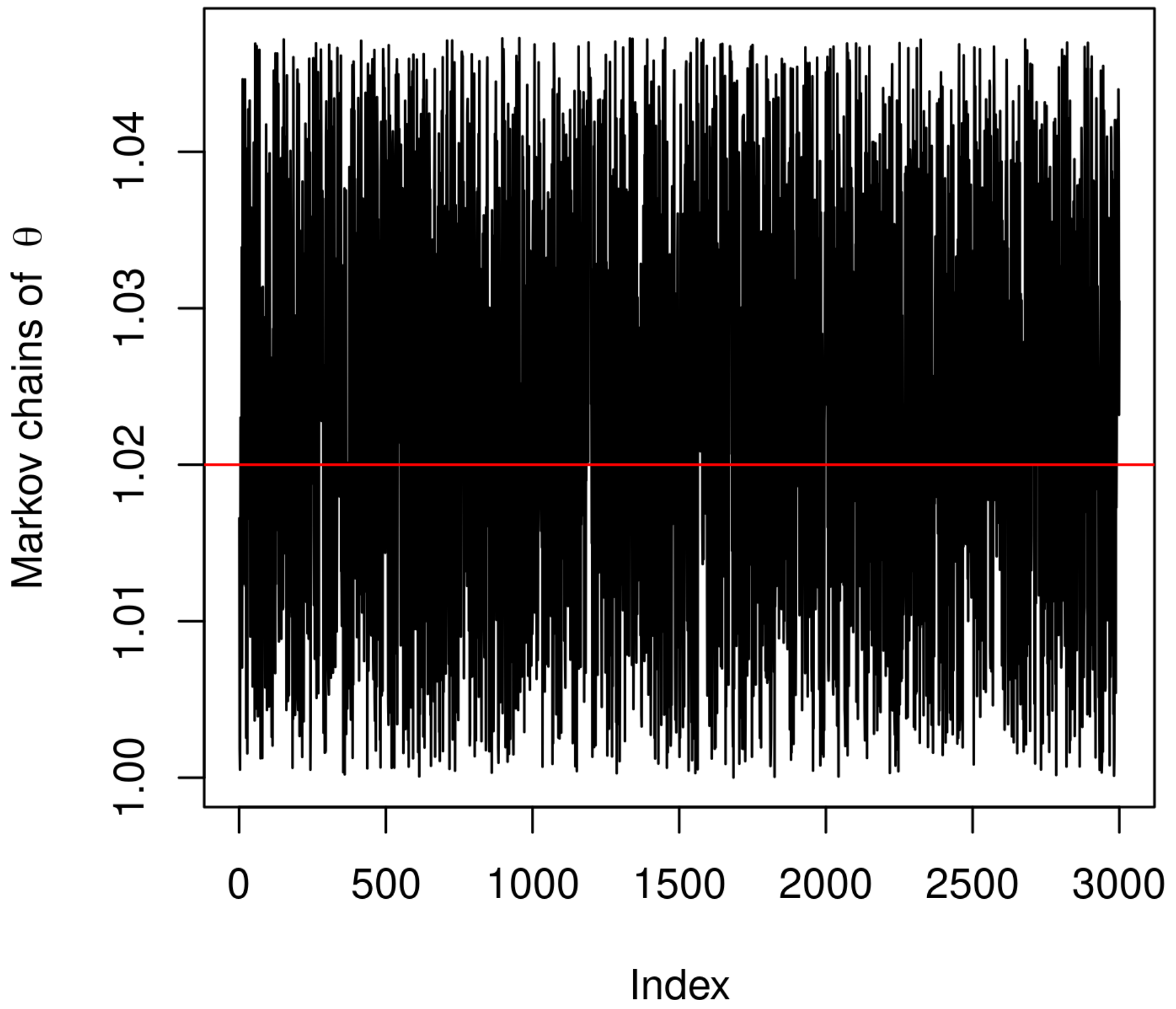
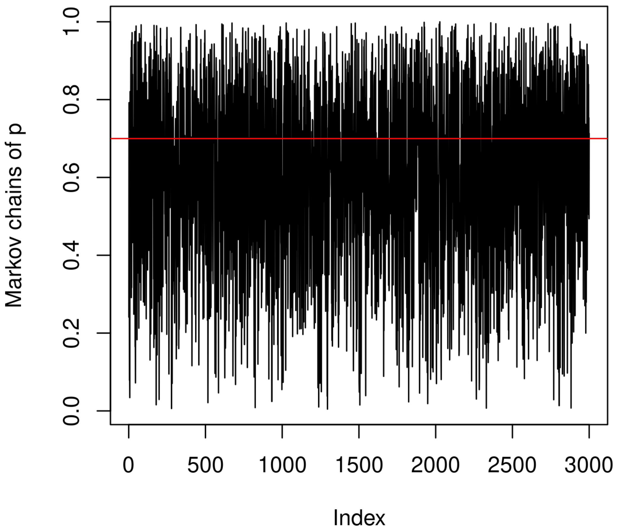
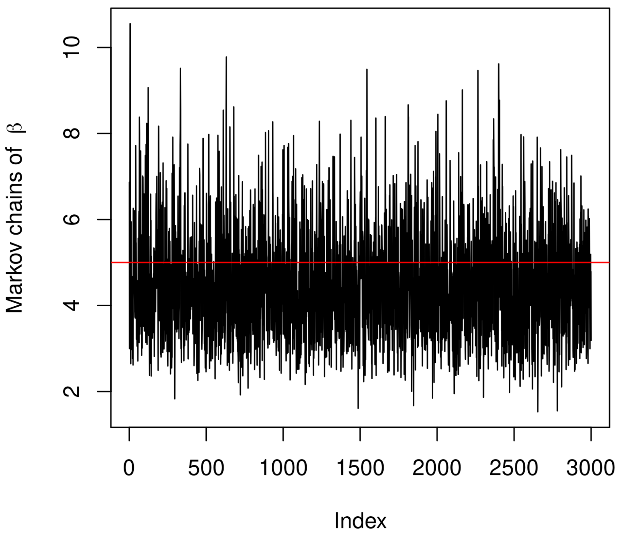
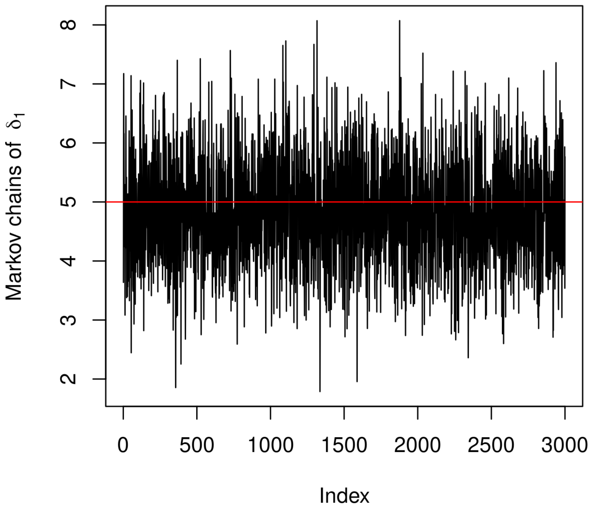
We found that the Markov chains of $\beta$ are highly correlated as their first-order autocorrelation coefficient is about 0.80, and the first-order autocorrelation coefficients of the other Markov chains of ${\delta }_1,{\delta }_2,\theta$ and p are smaller than 0.15. Therefore, we need to trim the Markov chains by spacing to reduce the autocorrelation among the Markov chains of $\beta$. To study the adequate interval length for spacing by simulations, we regenerate Markov chains of length $N=$ 31,000 and remove the first $N_1=$ 1000 chains for burn-in based on the SOS sample in Table 2 by using the proposed MH-GS MCMC method and check the first-order autocorrelation coefficient of the Markov chains of $\beta$ by spacing with the interval lengths of 1, 3, 5, 10, 15, and 20, respectively. We find that the spacing of interval length 10 can significantly reduce the first-order autocorrelation coefficient among the Markov chains of $\beta$ below 0.2. Based on the simulation findings, all Markov chains are slimmed by taking one of every 10 Markov chains to reduce the autocorrelation of Markov chains.

Figure 1, Figure 2, Figure 3, Figure 4 and Figure 5 present the 3000 slimmed Markov chains of $\beta ,{\delta }_1,{\delta }_2,\theta$ and p. In the scan of Figure 1, Figure 2, Figure 3, Figure 4 and Figure 5, we find that the proposed MH-GS MCMC method performs well to obtain the Bayes estimates of the CDS model parameters. The Bayes estimates are ${\widehat{\beta }}_B=4.471$, ${\widehat{\delta }}_1=4.826$, ${\widehat{\delta }}_2=9.706$, ${\widehat{\theta }}_B=1.023$, and ${\widehat{p}}_B=0.60$. All Markov chains well cover their true parameter. All the acceptance rates are high and reported by 0.715, 0.823, 0.95, 0.708, and 0.582 for the Markov chains of $\beta ,{\delta }_1,{\delta }_2,\theta$, and p, respectively. The first-order autocorrelation coefficients are 0.192, −0.001, 0.009, −0.004, and 0.058 for the slimmed Markov chains of $\beta ,{\delta }_1,{\delta }_2,\theta$, and p, respectively. Let $x=0.5$, it can be shown that the baseline survival function is $S_{g0}\left(x\right)=1-G_0\left(x\right)=0.669$ for $x=0.5$. The Markov chains of $S_{g0}(x=0.5)$ can be established through using the slimmed Markov chains of $\beta ,{\delta }_1,{\delta }_2,\theta ,p$ and Equation (8). The Bayes estimate of $S_{g0}(x=0.5)$ is ${\widehat{S}}_{g0,B}\left(x\right)=0.709$.

The Markov chains of $S_{g0}\left(x\right)$ can be used to establish the empirical distribution of ${\widehat{S}}_{g0,B}\left(x\right)$, and then the HCI and ECI of $S_{g0}\left(x\right)$ can be obtained. Based on the SOS sample in Table 2, the 95% HCI of $S_{g0}(x=0.5)$ is (0.588, 0.820) and the 95% ECI of $S_{g0}(x=0.5)$ is (0.581, 0.815). The coverage probabilities of the 95% HCI and ECI of $S_{g0}(x=0.5)$ are evaluated using the proposed MH-GS MCMC method with 1000 iterations. We obtain coverage probabilities of 0.961 and 0.974 for the HCI and ECI of $S_{g0}(x=0.5)$, respectively. The simulation results indicate that the coverage probability of HCI is closer to the nominal coverage probability than the coverage probability of ECI. Therefore, the HCI outperforms the ECI for the proposed MH-GS MCMC method in terms of the coverage probability.

4. Monte Carlo Simulations

To explore the estimation quality of the proposed Bayesian estimation method using an MH-GS MCMC approach, an intensive simulation study was conducted, and the proposed Bayesian estimation method is used to obtain the Bayes estimates of the CDS model parameters based on the SOS samples. As the parameter setting in Section 3, we consider the baseline of mBXIID $(\beta =5,{\delta }_1=5,{\delta }_2=10,p=0.7)$ for simulations with the parameters of $(n,r)=(30,15),(50,25),(80,30),(100,30),\theta =1.02$, and $p=0.2,0.3,0.5$. The CDS is defined as failure if half or over 30 of the components fail. We are also interested to evaluate the estimation quality of the proposed Bayesian estimation method for different mixture probabilities. We use $N=$ 31,000, $N_1=$ 1000, and interval length 10 for spacing to implement the MH-GS MCMC method. Moreover, the posterior distribution of $\pi (\Theta )$ in Equation (18) with the hyperparameters ${\eta }_1={\eta }_2={\eta }_3=1,k_1=\beta ,k_2={\delta }_1,k_3={\delta }_2,b_1=1$ and constant $b_2$ is used to obtain the Bayes estimates of the model parameters, where $b_2$ is the value when the hazard rate of CDS at the time of rth failure increases to 2 times of the baseline hazard rate. The proposals of ${\beta }^{*}\sim N({\beta }^{\left(i\right)},1^2)$, ${\delta }_1^{*}\sim N({\delta }_1^{\left(i\right)},1^2)$, ${\delta }_2^{*}\sim N({\delta }_2^{\left(i\right)},1^2)$, $p^{*}\sim N(p^{\left(i\right)},0.3^2)$, and ${\theta }^{*}\sim U(1,b_2)$ are used to generated the values of ${\beta }^{*},{\delta }_1^{*},{\delta }_2^{*},{\theta }^{*}$ and $p^{*}$ in Method I. If ${\beta }^{*}<0$, then ${\beta }^{*}={\beta }^{\left(i\right)}$; if ${\delta }_1^{*}\le 0$, then ${\delta }_i^{*}={\delta }_i^{\left(i\right)}$ for $i=1,2$; and if $p^{*}<0$ or $p^{*}>1$, then $p^{*}=p^{\left(i\right)}$.

We repeat the proposed Bayesian estimation method 10,000 times to obtain 10,000 Bayes estimates of $\beta ,{\delta }_1,{\delta }_2,\theta$ and p, then the 10,000 Bayes estimates are used to evaluate the bias and MSE for each Bayes estimate. Because the scales of the parameters are different, we use relative bias and relative square root of MSE, which are free of the scale, as the performance measures to study the estimation quality of the proposed Bayesian estimation method. The relative bias stands for the bias over the true parameter, and the relative square root of MSE stands for the square root of MSE over the true parameter. We use rBias and rsqMSE to denote the relative bias and relative square root of MSE for simplicity hereafter. All simulation results based on the proposed Bayesian estimation method are reported in

Table 3. The relative bias (rBias) and relative square root of the mean square error (rsqMSE) of Bayes estimates for $p=0.2$.

n	r		${\widehat{\mathit{\beta }}}_{\mathit{B}}$	${\widehat{\mathit{\delta }}}_{1\mathit{B}}$	${\widehat{\mathit{\delta }}}_{2\mathit{B}}$	${\widehat{\mathit{\theta }}}_{\mathit{B}}$	${\widehat{\mathit{p}}}_{\mathit{B}}$
30	15	rBiae	0.1032	−0.0279	−0.0134	0.0039	0.6278
		rsqMSE	0.1034	0.0281	0.0135	0.0039	0.6282
50	25	rBias	0.0953	0.0001	−0.0078	−0.0055	0.6083
		rsqMSE	0.0955	0.0032	0.0080	0.0055	0.6086
80	30	rBias	0.0275	0.0506	0.0194	−0.0060	0.6146
		rsqMSE	0.0280	0.0507	0.0195	0.0060	0.6149
100	30	rBias	−0.1522	0.0073	−0.0199	−0.0070	0.5168
		rsqMSE	0.1522	0.0079	0.0200	0.0070	0.5172

,

Table 4. The rBias and rsqMSE of Bayes estimates for $p=0.3$.

n	r		${\widehat{\mathit{\beta }}}_{\mathit{B}}$	${\widehat{\mathit{\delta }}}_{1\mathit{B}}$	${\widehat{\mathit{\delta }}}_{2\mathit{B}}$	${\widehat{\mathit{\theta }}}_{\mathit{B}}$	${\widehat{\mathit{p}}}_{\mathit{B}}$
30	15	rBias	0.0092	−0.0029	0.0359	0.0053	0.2283
		rsqMSE	0.0112	0.0044	0.0359	0.0053	0.2288
50	25	rBias	0.2052	−0.0036	−0.0421	−0.0053	0.2994
		rsqMSE	0.2054	0.0047	0.0422	0.0053	0.2997
80	30	rBias	0.3267	0.0425	0.0054	−0.0099	0.2757
		rsqMSE	0.3268	0.0426	0.0057	0.0099	0.2761
100	30	rBias	0.0895	−0.0443	0.0009	−0.0086	0.2236
		rsqMSE	0.0897	0.0444	0.0019	0.0086	0.2241

and

Table 5. The rBias and rsqMSE of Bayes estimates for $p=0.5$.

n	r		${\widehat{\mathit{\beta }}}_{\mathit{B}}$	${\widehat{\mathit{\delta }}}_{1\mathit{B}}$	${\widehat{\mathit{\delta }}}_{2\mathit{B}}$	${\widehat{\mathit{\theta }}}_{\mathit{B}}$	${\widehat{\mathit{p}}}_{\mathit{B}}$
30	15	rBias	0.0697	−0.0113	0.0217	0.0041	0.0035
		rsqMSE	0.0701	0.0118	0.0217	0.0041	0.0099
50	25	rBias	−0.0310	0.0114	−0.0155	−0.0044	−0.0167
		rsqMSE	0.0315	0.0118	0.0156	0.0044	0.0192
80	30	rBias	−0.2359	<0.0001	0.0165	−0.0075	−0.0646
		rsqMSE	0.2359	0.0029	0.0166	0.0075	0.0653
100	30	rBias	0.1844	−0.0119	0.0060	−0.0066	0.0442
		rsqMSE	0.1845	0.0122	0.0062	0.0066	0.0452

.

In order to compare the estimation performance of the proposed Bayesian estimation method with the maximum likelihood estimation method, the MLEs of $\beta ,{\delta }_1,{\delta }_2,\theta$, and p are also obtained and denoted by $\widehat{\beta },\widehat{{\delta }_1},\widehat{{\delta }_2},\widehat{\theta }$, and $\widehat{p}$, respectively. Moreover, the rBias and rsqMSE of each MLE are evaluated based on 10,000 obtained MLEs. Because there is a high probability that the gradient methods cannot successfully solve log-likelihood equations to obtain the MLEs of model parameters, we use the proposed Bayesian estimation method with a non-informative prior distribution to obtain approximate MLEs. Let ${\kappa }_1={\kappa }_2={\kappa }_3=100$ and ${\eta }_1={\eta }_2={\eta }_3=1$ in Equation (17) to make the Gamma distributions of $\beta$, ${\delta }_1$, and ${\delta }_2$ have a big variance, and then the prior distribution of Equation (17) becomes non-informative. All simulation results based on the maximum likelihood estimation method are reported in

Table 6. The rBias and rsqMSE of maximum likelihood estimates (MLEs) for $p=0.2$.

n	r		$\widehat{\mathit{\beta }}$	${\widehat{\mathit{\delta }}}_1$	${\widehat{\mathit{\delta }}}_2$	$\widehat{\mathit{\theta }}$	$\widehat{\mathit{p}}$
30	15	rBias	5.3671	0.0603	0.0549	−0.0179	−0.7863
		rsqMSE	5.3673	0.0604	0.055	0.0179	0.7863
50	25	rBias	5.5802	0.1087	0.0203	−0.0185	−0.8204
		rsqMSE	5.5804	0.1087	0.0204	0.0185	0.8205
50	30	rBias	3.3028	0.0643	0.0206	−0.0187	−0.8855
		rsqMSE	3.3029	0.0644	0.0207	0.0187	0.8855
100	30	rBias	4.2000	0.0955	0.0556	−0.0185	−0.8890
		rsqMSE	4.2001	0.0955	0.0557	0.0185	0.8891

,

Table 7. The rBias and rsqMSEs of MLEs for $p=0.3$.

n	r		$\widehat{\mathit{\beta }}$	${\widehat{\mathit{\delta }}}_1$	${\widehat{\mathit{\delta }}}_2$	$\widehat{\mathit{\theta }}$	$\widehat{\mathit{p}}$
30	15	rBias	7.8958	0.0631	0.0374	−0.0174	−0.8314
		rsqMSE	7.8961	0.0632	0.0374	0.0174	0.8315
50	25	rBias	5.0357	0.0586	0.0811	−0.0184	−0.8866
		rsqMSE	5.0358	0.0587	0.0811	0.0184	0.8867
50	30	rBias	2.9665	0.0719	0.0419	−0.0187	−0.9196
		rsqMSE	2.9665	0.0720	0.0419	0.0187	0.9197
100	30	rBias	4.7010	0.0766	0.0574	−0.0188	−0.9245
		rsqMSE	4.7011	0.0766	0.0574	0.0188	0.9245

and

Table 8. The rBias and rsqMSEs of MLEs for $p=0.5$.

n	r		$\widehat{\mathit{\beta }}$	${\widehat{\mathit{\delta }}}_1$	${\widehat{\mathit{\delta }}}_2$	$\widehat{\mathit{\theta }}$	$\widehat{\mathit{p}}$
30	15	rBias	6.5672	0.1020	0.0448	−0.0175	−0.8937
		rsqMSE	6.5674	0.1021	0.0448	0.0175	0.8937
50	25	rBias	4.5287	0.0565	0.0442	−0.0182	−0.9311
		rsqMSE	4.5288	0.0567	0.0442	0.0182	0.9312
50	30	rBias	5.6215	0.0777	0.0278	−0.0186	−0.9380
		rsqMSE	5.6216	0.0778	0.0279	0.0186	0.9381
100	30	rBias	4.4166	0.1011	0.0533	−0.0188	−0.9485
		rsqMSE	4.4167	0.1012	0.0534	0.0188	0.9485

. In view of Table 3, Table 4, Table 5, Table 6, Table 7 and Table 8, we find the following results.

• The Bayes estimates in Table 3, Table 4 and Table 5 are more reliable and outperform the MLEs in Table 5, Table 6 and Table 7 in terms of the measures of bias and MSE. The rBias and rsqMSE of the Bayes estimate are smaller than the rBias and rsqMSE of MLE.
• The estimation results in Table 3, Table 4 and Table 5 indicate that the estimation quality of the Bayes estimate for the mixture proportion is worse than the estimation quality of the Bayes estimates for other parameters. Moreover, the censoring rate significantly influences the estimation quality of Bayes estimates.
• The maximum likelihood estimation method is less reliable for estimating the mixture proportion and shape parameter. Moreover, the acceptance rate is low for the Markov chains of the parameters of $\theta$ and p if non-informative prior is used to implement the Bayesian estimation methods. The rBias and rsqMSE of the MLEs of $\beta$ and p in Table 6, Table 7 and Table 8 are large even when the sample size increases to 100 or the censoring rate is high. The findings mean that it could fail to use the maximum likelihood estimation method to obtain reliable estimates of the model parameters if the component lifetimes in CDS follow a baseline mixture distribution.

5. Conclusions

In this study, we proposed a maximum likelihood estimation method and a Bayesian estimation procedure using the MH-GS MCMC approach to obtain reliable Bayes estimators of the CDS model parameters and baseline survival function based on SOS samples when the component lifetimes follow the baseline of mixture-BXIID. The PTHR function is used to characterize the increased system hazard caused by component failures. For each component failure, the stress loading can be equally redistributed to the surviving components in the CDS. The proposed methods include the Bayesian estimation for a single baseline of BXIID for CDS as special case when $p=1$.

The implementation of the proposed Bayesian estimation method with the MH-GS MCMC approach is presented systematically in Method I. The proposed Bayesian estimation method is studied by utilizing a numerical example. An intensive simulation study is conducted to evaluate the performance of the proposed Bayesian estimation method and the maximum likelihood estimation method. Based on the simulation results in Section 4, we find that the proposed Bayesian estimation method outperforms the maximum likelihood estimation method to obtain reliable estimates of the CDS model parameters and its baseline survival function in terms of the relative bias and MSE.

The maximum likelihood estimation method does not perform well in obtaining reliable MLEs of the shape parameter and mixture proportion, and it is also intractable to obtain the Fisher information matrix to construct an approximate confidence interval for the baseline survival function of mixture-BXIID. Therefore, one major contribution of this study is to propose a simple Bayesian estimation method to overcome the divergence problem of the typical maximum likelihood estimation method to obtain approximate MLEs using a non-informative prior distribution. Moreover, the proposed HCI and ECI methods based on using the Markov chains of the baseline survival function can help practitioners to carry out interval inference for the baseline survival function.

The simulation results in Section 4 also show that the estimation quality of the Bayes estimate for the mixture proportion is worse than the estimation quality of the Bayes estimates for other parameters. Moreover, the censoring rate significantly influences the estimation quality of Bayes estimates. When the censoring rate is low, the rBias and rsqMSE of the Bayes estimate could be less stable and fail to decrease along the sample size. There is also room to improve the estimation quality of using the proposed Bayesian estimation method to estimate the shape parameter of the mixture-BXIID. It is also important to extend the proposed Bayesian estimation method to other mixture distributions. These topics can be studied in the future.

References

1. Kamps, U. A concept of generalized order statistics. J. Stat. Plan. Inference 1995, 48, 1–23. [Google Scholar] [CrossRef]
2. Cramer, E.; Kamps, U. Sequential order statistics and k-out-of-n systems with sequentially adjusted failure rates. Ann. Inst. Stat. Math. 1996, 48, 535–549. [Google Scholar] [CrossRef]
3. Cramer, E.; Kamps, U. Estimation with sequential order statistics from exponential distributions. Ann. Inst. Stat. Math. 2001, 53, 307–324. [Google Scholar] [CrossRef]
4. Cramer, E.; Kamps, U. Marginal distributions of sequential and generalized order statistics. Metrika 2003, 58, 293–310. [Google Scholar] [CrossRef]
5. Revathy, S.A.; Chandrasekar, B. Equivariant estimation of parameters based on sequential order statistics from (1,3) and (2,3) Systems. Commun. Stat. Theory Methods 2007, 36, 541–548. [Google Scholar] [CrossRef]
6. Zhuang, W.; Hu, T. Multivariate stochastic comparisons of sequential order statistics. Probab. Eng. Inform. Sci. 2007, 21, 47–66. [Google Scholar] [CrossRef]
7. Balakrishnan, N.; Beutner, E.; Kamps, U. Modeling parameters of a load-sharing system through link functions in sequential order statistics models and associated inference. IEEE Trans. Reliab. 2011, 60, 605–611. [Google Scholar] [CrossRef]
8. Burkschat, M. Systems with failure-dependent lifetimes of components. J. Appl. Probab. 2009, 46, 1052–1072. [Google Scholar] [CrossRef] [Green Version]
9. Beutner, E.; Kamps, U. Order restricted statistical inference for scale parameters based on sequential order statistics. J. Stat. Plan. Inference 2009, 139, 2963–2969. [Google Scholar] [CrossRef]
10. Deshpande, J.V.; Dewan, I.; Naik-Nimbalkar, U.V. A family of distributions to model load sharing systems. J. Stat. Plan. Inference 2010, 140, 1441–1451. [Google Scholar] [CrossRef]
11. Beutner, E. Nonparametric model checking for k-out-of-n systems. J. Stat. Plan. Inference 2010, 140, 626–639. [Google Scholar] [CrossRef]
12. Bedbur, S. UMPU tests based on sequential order statistics. J. Stat. Plan. Inference 2010, 140, 2520–2530. [Google Scholar] [CrossRef]
13. Schenk, N.; Burkschat, M.; Cramer, E.; Kamps, U. Bayesian estimation and prediction with multiply Type-II censored samples of sequential order statistics from one- and two-parameter exponential distributions. J. Stat. Plan. Inference 2011, 141, 1575–1587. [Google Scholar] [CrossRef]
14. Navarro, J.; Burkschat, M. Coherent systems based on sequential order statistics. Nav. Res. Log. 2011, 58, 123–135. [Google Scholar] [CrossRef]
15. Balakrishnan, N.; Kamps, U.; Kateri, M.A. Sequential order statistics approach to step-stress testing. Ann. Inst. Stat. Math. 2012, 64, 303–318. [Google Scholar] [CrossRef]
16. Burkschat, M.; Navarro, J. Dynamic signatures of coherent systems based on sequential order statistics. J. Appl. Probab. 2013, 50, 272–287. [Google Scholar] [CrossRef]
17. Burkschat, M.; Torrado, N. On the reversed hazard rate of sequential order statistics. Stat. Probabil. Lett. 2014, 85, 106–113. [Google Scholar] [CrossRef]
18. Park, C. Parameter estimation from load-sharing system data using the expectation-maximization algorithm. IIE Trans. 2013, 45, 147–163. [Google Scholar] [CrossRef]
19. Bedbur, S.; Burkschat, M.; Kamps, U. Inference in a model of successive failures with shape-adjusted hazard rates. Ann. Inst. Stat. Math. 2016, 68, 639–657. [Google Scholar] [CrossRef]
20. Sutar, S.S.; Naik-Nimbalkar, U.V. Accelerated failure time models for load sharing systems. IEEE Trans. Reliab. 2014, 63, 706–714. [Google Scholar] [CrossRef]
21. Esmailian, M.; Doostparast, M. Estimation based on sequential order statistics with random removals. Probab. Math. Stat. 2014, 34, 81–95. [Google Scholar]
22. Shafay, R.; Balakrishnan, N.; Sultan, K.S. Two-sample Bayesian prediction for sequential order statistics from exponential distribution based on multiply Type-II censored samples. J. Stat. Comput. Simul. 2014, 84, 526–544. [Google Scholar] [CrossRef]
23. Hashempour, M.; Doostparast, M. Estimation with non-homogeneous sequential k-out-of-n system lifetimes. Reliab. Theory Appl. 2015, 49, 49–52. [Google Scholar]
24. Bedbur, S.; Kamps, U.; Kateri, M. Meta-analysis of general step-stress experiments under repeated type-II censoring. Appl. Math. Model. 2015, 39, 2261–2275. [Google Scholar] [CrossRef]
25. Balakrishnan, N.; Jiang, N.; Tsai, T.R.; Lio, Y.L.; Chen, D.G. Reliability Inference on composite dynamic systems based on Burr type-XII distribution. IEEE Trans. Reliab. 2015, 64, 144–153. [Google Scholar] [CrossRef]
26. Hashempour, M.; Doostparast, M. Statistical evidences in sequential order statistics arising from a general family of lifetime distributions. Istatistik 2016, 9, 29–41. [Google Scholar]
27. Burkschat, M.; Cramer, E.; Górny, J. Type-I censored sequential k-out-of-n systems. Appl. Math. Model 2016, 40, 8156–8174. [Google Scholar] [CrossRef]
28. Hashempour, M.; Doostparast, M. Bayesian inference on multiply sequential order statistics from heterogeneous exponential populations with GLR test for homogeneity. Commun. Stat. Theory Methods 2017, 46, 8086–8100. [Google Scholar] [CrossRef]
29. Baratnia, M.; Doostparast, M. Modelling lifetime of sequential r-out-of-n systems with independent and heterogeneous components. Commun. Stat. Simul. Comput. 2017, 46, 7365–7375. [Google Scholar] [CrossRef]
30. Burkschat, M.; Navarro, J. Ageing properties of sequential order statistics. Probab. Eng. Inform. Sci. 2011, 25, 1–19. [Google Scholar] [CrossRef]
31. Barakat, H.M.; Nigm, E.M.; El-Adll, M.E.; Yusuf, M. Prediction of future generalized order statistics based on exponential distribution with random sample size. Stat. Pap. 2018, 59, 605–631. [Google Scholar] [CrossRef]
32. Katzur, A.; Kamps, U. Classification using sequential order statistics. Adv. Data Anal. Classif. 2020, 14, 201–230. [Google Scholar] [CrossRef]
33. Tsai, T.R.; Xin, H.; Kao, C.H. Bayesian estimation based on sequential order statistics for heterogeneous baseline Gompertz distributions. Mathematics 2021, 9, 145. [Google Scholar] [CrossRef]
34. Tsai, T.R.; Ng, H.K.; Pham, H.; Lio, Y.L.; Chiang, J.Y. Reliability inference for VGA adapter from dual suppliers based on contaminated type-I interval-censored data. Qual. Reliab. Eng. Int. 2019, 35, 2297–2313. [Google Scholar] [CrossRef]
35. Robert, C.P. The Metropolis-Hastings Algorithm. In Wiley StatsRef: Statistics Reference Online; Wiley: Hoboken, NJ, USA, 2016. [Google Scholar]
Figure 1. The Markov chains of β . The horizontal line is the true value of β .
Mathematics 09 00810 g001
Figure 2. The Markov chains of δ 1 . The horizontal line is the true value of δ 1 .
Mathematics 09 00810 g002
Figure 3. The Markov chains of δ 2 . The horizontal line is the true value of δ 2 .
Mathematics 09 00810 g003
Figure 4. The Markov chains of θ . The horizontal line is the true value of θ .
Mathematics 09 00810 g004
Figure 5. The Markov chains of p. The horizontal line is the true value of p.
Mathematics 09 00810 g005