Abstract
In this paper we modify a standard SIR model used to study the spread of some diseases by incorporating a disease that destroys the immunity that is conferred by having one of the other diseases or being vaccinated against the disease. A specific biological example of this occurs with measles. Studies of recent measles’ patients has shown that many patients have lost some (or all) of their immunity to other diseases from which they were previously protected. In the future, models like those developed here might be helpful in understanding how viruses that affect multiple organ systems can impact the effect the disease has on at risk populations.
1. Introduction
Many viral diseases such as measles, chicken pox, mumps, smallpox, and so on confer immunity to the survivor of the disease. Unfortunately, diseases such as these can inflict serious damage on the infected individual, including death, as well as being spread to uninfected individuals who come in contact with infected ones. Consequently, it is a top priority of nearly all health organizations to vaccinate as many individuals as possible against diseases such as those mentioned here. For example, smallpox is a lethal (30% death rate) and highly contagious disease. Due to a well-documented global immunization campaign, the last documented case of smallpox occurred in Somalia in 1977 and, subsequently, smallpox was declared eradicated in 1980. As a consequence, individuals are no longer vaccinated against smallpox. (The interested reader may study the ramifications of this policy. Some have worried that the smallpox virus could be used as a biological weapon. As a consequence, it is theorized that many governments have stockpiled smallpox vaccines to prevent a global pandemic in the event that there was an attack using a virus such as smallpox as the weapon.) However, it is not known what percent of the population that was vaccinated against smallpox is still immune to smallpox. Thus, if a disease such as measles destroys immunity to existing diseases, if a person contracted measles and transmitted the infection to various individuals immune to smallpox, the measles infection might destroy their immunity to smallpox creating the possibility of a smallpox epidemic. The eradication of smallpox, which is frequently thought to be the only disease eradicated, is readily available. The Centers for Disease Control and Prevention provides a comprehensive overview of smallpox which you can access by pointing your browser to https://www.cdc.gov/smallpox/index.html (accessed on 7 April 2021).
For example, recently measles has seen outbreaks throughout the United States that have led to local epidemics that have been documented in scientific literature [1], as well as observed in popular media [2]. Additionally, recent research indicates that although surviving measles confers immunity to measles, having measles may damage and/or destroy the immunity to other diseases that was obtained by surviving infection or vaccination. For a few examples, refer to articles by Mina et al. [3], Petrova et al. [4], Griffin [5], or Kelland [6].
The phrase as many individuals deserves special explanation. Mathematical models studying the spread of diseases are classified into a variety of different groups. A few such groups include
- Susceptible-infected-susceptible (SIS). After an individual has the disease and recovers from the disease, they are again susceptible to the disease. Many bacterial infections (such as strep throat and many sinus infections) are frequently included in this category.
- Susceptible-infected-recovered (SIR). After an individual has had the disease, they are no longer susceptible to the disease. Many viral infections (such as measles and chickenpox) are frequently included in this category because if an individual recovers from the disease, they are immune to subsequent occurrences of the disease.
This list is quite limited. Mathematical models take a variety of forms that take into consideration many variables such as including not taking births and deaths (without vital dynamics) or taking births and deaths (with vital dynamics) into consideration. In mathematical models such as these, the phrase as many individuals is quantified by a number, typically denoted as , which is called the basic reproductive ratio. The basic reproductive ratio, , is defined in different ways depending upon the context of the problem under consideration. We use Britton’s [7], definition. In the context of a disease that may be spread through a population by an individual’s contact with another, often is interpreted to mean the percentage of the population of individuals that need to be vaccinated so that an infected individual is not statistically likely to interact with a susceptible individual and, consequently, increase the spread of the disease. In situations such as this, the percentage that needs to be vaccinated to prevent the disease from being spread among the population is referred to as herd immunity and used interchangeably with basic reproductive ratio. Refer to introductory mathematical biology texts such as Britton [7], for a comprehensive introduction to mathematical biology and the vocabulary used here.
The value of to achieve herd immunity is very important. If the fraction vaccinated against a disease is less than its -value, the disease may become epidemic, a “widespread” occurrence of an infectious disease at a particular time, or endemic, regularly occurring or persistent, in the population. For many health-related issues there are reasons why some individuals cannot be vaccinated for various diseases. On the other hand, some individuals choose to not vaccinate for other reasons. Adding the two groups may result in the fraction of the population being vaccinated against a particular disease may result in the fraction of the population vaccinated less than its -value. Once the fraction of the population vaccinated is below its -value, epidemics and/or endemics can arise.
Many of the terms and concepts presented here were first introduced in the article that forms the foundations for the mathematical models of epidemics by Kermack and McKendrick [8], in 1927, which we summarize next.
2. Summary of the Basic SIR Model without Vital Dynamics
We summarize the case when the disease under consideration spreads and confers immunity, as is the case with many viral infections, such as chickenpox mentioned above, that was discussed by Kermack and McKendrick [8], for completeness purposes. In this situation, we have a susceptible (S), infected (I), and recovered (R) population where it is assumed that the R population is immune from contracting the disease again, such as is suspected with viral diseases such as measles. Without taking vital dynamics (such as births and deaths) into consideration, we assume that the population is closed with constant size N so that
Schematically we have
so the model takes the form
In this model, represents the proportion of interactions that result in I infections, often referred to as the (pairwise) infectious contact rate, and represents the rate of recovery. In the subsequent discussion, the interpretations of the constants remain the same however we use subscripts to denote relationships between the , , and classes of the population. Now we non-dimensionalize the equations by letting
The equations become
where is the basic reproductive ratio. Observe that if , then as so . On the other hand, if , then as . For
we have two rest points and . The Jacobian for system (3) is
Evaluated at , the Jacobian
has eigenvalues and . Thus, is stable, but not asymptotically stable. On the other hand, evaluated at the Jacobian is
which has eigenvalues and . Once again, the equilibrium point is stable, but not asymptotically stable. The two situations are illustrated in Figure 1. In (a), while in (b) .
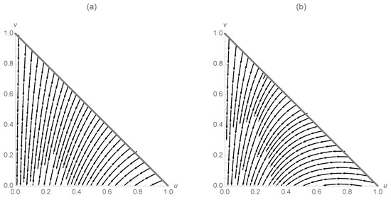
Figure 1.
(a) Trajectories for and (b) trajectories for .
It is important to note that the scaling performed on system (1) cannot be performed if the population is not assumed to be constant, which would be the case if vital dynamics (such as births, deaths, immigration, emigration, and so on) were taken into consideration.
3. Summary of the Basic SIR Model with Vital Dynamics
An SIR model that takes basic vital dynamics (births and deaths) into consideration is
where B is interpreted to be a constant birth rate, d is the natural death rate, c is the disease induced death rate, and , where N represents the total population. Refer to texts like [7] or [9]. and have the same interpretations as before. Adding the three equations in system (4) gives us
Because is not constant, it is not possible to perform the same scaling to dimensionless variables as with system (1).
Because of the equation , we can analyze any three of the equations. We follow Britton’s convention [7], and choose to analyze the equations.
We first find the rest points (equilibrium points) of system (6) by solving
resulting in
and
where (the basic reproductive ratio [7]) takes the form
to make infectious contacts and
Comment: One interpretation of is that it is a number that guarantees that will be unstable so that the diseases persists (i.e., is endemic) as shown in the following calculation.
The Jacobian of system (6) is
Evaluated at , the Jacobian is
with eigenvalues , and
To guarantee that is unstable, we will further assume that
On the other hand, evaluated at (assuming that exists) the Jacobian is
with eigenvalues and . is stable when it exists. See Figure 2. In the figure, (total population) is in black, (the susceptible population) is in gray, and (the infected population) is in dashed gray. Observe in (a) that the disease dies out so that . On the other hand, in (b) the disease is endemic in the form of a stable equilibrium point. That is, the prevalence of each class is constant.
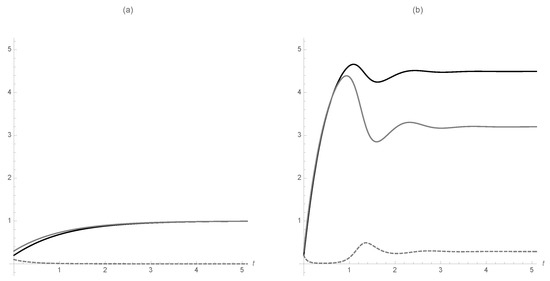
Figure 2.
(a) The disease dies out. (b) The disease is endemic in the population at a constant rate. (In the figure S is in black, I is in gray, and R is dashed).
4. Two Infectious SIR Diseases Where One Disease Destroys Immunity to the Other Endemic to the Population
To consider two infectious SIR diseases, we first rewrite system (4) as two systems, using the subscripts one and two, respectively, to separate the two diseases. The birth rates and natural death rates (B and d) are assumed to be the same for each disease. The notation is the same as that used previously: denotes the portion of the population susceptible to disease i, denotes the portion of the population infected by disease i, and denotes the portion of the population recovered from disease i.
We will assume that the second disease destroys immunity to the first. To form the model, we introduce three additional variables, , , and . The interpretations of the nine dependent variables change slightly
- The Equations.
- -
- represents the portion of the population that is susceptible to disease one but not disease two. The population increases as those in the and the populations recover.
- -
- represents the portion of the population that were initially in the group but are now infected.
- -
- represents the portion of the population that were initially in the group but are now recovered.
- The Equations.
- -
- represents the portion of the population that is susceptible to disease two but not disease one.
- -
- represents the portion of the population that were initially in the group but are now infected.
- -
- represents the portion of the population that were initially in the group but are now recovered.
- The Equations.
- -
- represents the portion of the population that is susceptible to diseases one and two. The growth rate of is assumed to be constant, B, but those in the class move to the and classes, and classes, or class.
- -
- represents the portion of the population that were initially in the group but are now infected by both diseases. Those in the class who survive the disease move to the class.
- -
- represents the portion of the population that were initially in the group but are now recovered from both diseases. Those in the class move to the class, which models the destruction of immunity to the first disease by the second disease.
With the above in mind, we start by forming the equation using the standard equations, (8) as a guide. The interpretations of the constants remain the same.
All are born into the class. The susceptibles are born into the class and then removed to class and , and , or so the equation takes the form
where the constants have the same interpretation as discussed previously. The equations for the infected and recovered portions of the population are nearly the same, other than the growth rates might differ with this model.
The equation takes into consideration the infectives to both the first and second diseases. An individual can become a member of the class by an interaction. Once an individual recovers from both diseases they move to the class and the class because the second diseases destroys immunity to the first disease.
Observe that an interaction could result in an or infection, as well. Similarly, it is possible that an and simultaneously could occur that would result in an infection. For now, we will assume that the number of , , and infections as a result of such interactions is small enough to be ignored but will be revisited in a later study.
If an individual moves into the class then they move into the class and if an individual moves into the class they move into the class. Thus,
We now turn our attention to the equation: the individuals susceptible to the first disease. These are individuals who have contracted the second disease but not the first so moved to class . However, because we are assuming that the second disease destroys immunity to the first, the class also includes the survivors of the second disease which are included in the class. Thus, the equation takes the form
Combining Equations (9)–(12) yields the system of interest.
where all the initial conditions are nonnegative and at least one initial condition is positive. The , , , and d terms have the same interpretation as discussed previously. Because the second disease destroys immunity to the first we consider it to be the more “dangerous” disease.
A diagram of the model is shown in Figure 3.
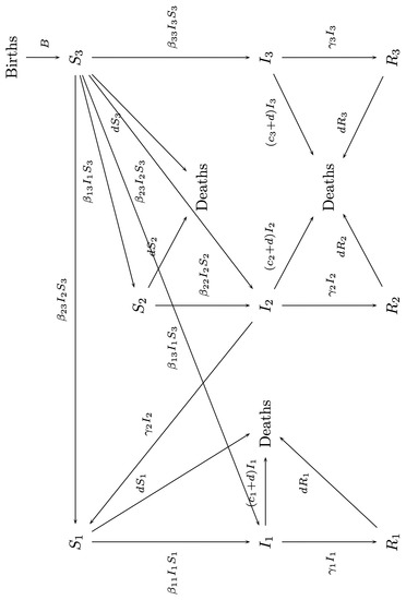
Figure 3.
A diagram of the dynamics modeled by system (13).
5. The Boundary Rest Points
Observe that if , then it is not possible for to be a rest point. Boundary rest points of interest occur if and or if , , and . Note that if and then and .
- , ; ,
If and (and/or and ), solving
results in , (and/or , ), , and , which we will denote as
We define . A second equilibrium point is
The Jacobian of system (13) evaluated at is
with eigenvalues
for , 2, and 3 and then . Thus, will be stable when
B (the constant birth rate) and d (the natural death rate are constant for all three populations). The disease induced death rates, , are assumed to be different as well as the recovery rates, . The transmission coefficients for moving from the class to the class are given by . In (15), we assume that is the largest of these three numbers: being susceptible to both diseases is more risky than being susceptible to only one of them.
With the interpretation of the variables in mind, we solve for when
as follows.
The results coincide with what most would predict: the diseases are eliminated when the transmission coefficients (contact rates) are sufficiently small.
If is stable, both diseases are eliminated from the population. Observe that exists if is unstable (otherwise, the -component is negative). If exists, the Jacobian of system (13) evaluated at is
with eigenvalues for , 2, and
In the numerical examples, we have chosen parameter values that illustrate the variety of situations and outcomes that we observed. Because the variables are dimensionless, we cannot use real data here.
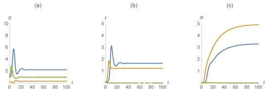
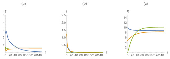
Example 1.
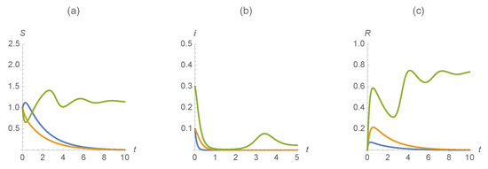
Our first example illustrates a scenario with , , , , , , . Figure 4 indicates that in the case when individuals are susceptible, infected, and recovered from both diseases persist while the cases when individuals are susceptible, infected, and recovered from one disease are eliminated.
Figure 4.
(a) , (b) , and (c) . The first disease is represented in blue, the second in orange and those susceptible/infected/recovered by diseases in green.
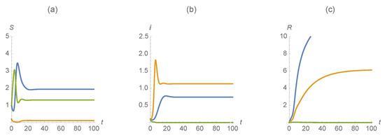
Example 2.
Our second example illustrates a scenario with , , , , , , , , , . Figure 5 indicates that in the case when individuals are susceptible, infected, and recovered from one of the diseases persist while the cases when individuals are susceptible, infected, and recovered from both diseases are eliminated.
Figure 5.
(a) , (b) , and (c) . The first disease is represented in blue, the second in orange and those susceptible/infected/recovered by diseases in green.
The two examples reveal the extremes possible as well as some of the limitations of the model.
6. Simple Vaccination
System (13) does not take vaccination against the disease into consideration. We will assume that vaccination of an individual in the class moves the individual to the class. Let denote the vaccination rate of the population . For example, denotes the vaccination rate of the the population against both diseases. Then, system (13) becomes
where all the initial conditions are nonnegative and at least one initial condition is positive. The , , , and d terms have the same interpretation as discussed previously.
The most desirable outcome is that . It is not possible for but , but , but or that exactly one of , , or but the other two infection rates do not. In any of these situations, the only rest points have at least one negative component, which is not meaningful in the context of the discussion as we are discussing populations sizes which must be greater than or equal to zero.
The Jacobian of system (18) is
where and .
The most desirable outcome is that both diseases are eliminated. In the case that , system (18) has a single rest point
Evaluated at , is
with eigenvalues , , , , , , and .
Observe that will be stable when are all negative, which occurs if
In the same manner as in Equation (15), in inequality (19), we assume that is the largest of these three numbers because being susceptible to both diseases creates more risk than only be susceptible to one of them. We are assuming that the transmission rate is greater for those susceptible to both diseases rather than those susceptible to only one. (Thus, we are fundamentally assuming that a single vaccination against both diseases is more desirable than multiple vaccinations against several.)
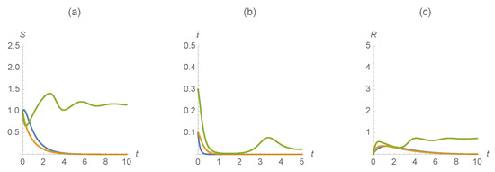
Example 3.
The first example uses the parameter values , , , , , , , , , . Figure 6 indicates the dramatic difference of how vaccination changes the outcome. With this scenario, we see that individuals infected with one of the diseases persist while those infected with both are not. On the other hand, using the same parameter values without vaccination we saw that the infectives with both diseases persisted.
Figure 6.
(a) , (b) , and (c) . The first disease is represented in blue, the second in orange and those susceptible/infected/recovered by diseases in green.
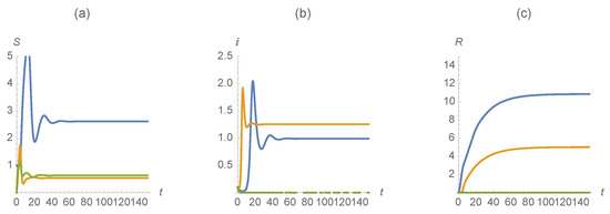
Example 4.
Next we use the parameter values , , , , , , , , , , . Figure 7 indicates the dramatic difference of how vaccination changes the outcome. With this scenario, we see that individuals infected with both of the diseases persist while infected with one are not, even with very high vaccination rates for both the and populations.
Figure 7.
(a) , (b) , and (c) . The first disease is represented in blue, the second in orange and those susceptible/infected/recovered by diseases in green.
Example 5.

Finally, we illustrate a desired solution that comes with a “cost." We illustrate with the parameter values , , , , , , , , , , . Observe that the “cost" is the portion of vaccinations of to the group to achieve elimination of both diseases. Figure 8 illustrates that if the population is illustrated at a very high rate, both diseases can be eradicated from the population.
Figure 8.
(a) , (b) , and (c) . The first disease is represented in blue, the second in orange and those with susceptible/infected/recovered by diseases in green.
7. Selective Vaccination
One of the main limitations of the model represented by system (18) is that is the vaccination rate of the population class and moves them from the class to the class. We propose a different vaccination scheme that might be more realistic in many situations as follows.
- (1)
- We assume that the first disease (modeled with the equations) is well understood and that the population is vaccinated at a high enough rate to achieve herd immunity. Thus the population class is vaccinated against the first disease so a portion of the class moves to the class and the class. This is represented by a term in the population that is then added to the and equations in system (20).
- (2)
- The second disease (modeled with the equations) is not well understood but is considered to be more harmful than the first disease. Some ways it might be more harmful are listed as follows,
- The second disease may have a higher death rate than the first disease.
- The second disease may destroy the immunity conferred by either having the first disease or being vaccinated against the first disease.
- (3)
- Once the second disease is understood, those in the class are vaccinated against the second disease and those in the class are vaccinated against both the first and second diseases. In system (20), this is represented by the term in the equation that is then added to the equation in the same way as in (18). The term now has the same interpretation as it did in system (18).
These assumptions are taken into consideration with
where all the initial conditions are nonnegative and at least one initial condition is positive. The , , , and d terms have the same interpretation as discussed previously.
The Jacobian of system (20) is -4.6cm0cm
where and .
- .
If we obtain the rest point
We now abbreviate with . Evaluated at , is
with eigenvalues , , , , , , and
Finding reasonable conditions for which all the eigenvalues, particular are negative so that is stable is difficult. Nevertheless, examples can indicate some of the possible outcomes.
Example 6.
We choose parameter values similar to those used in the previous examples. Here, , , , , , , , , , , , , and . These parameter values are interpreted to mean that a large portion of the population is vaccinated against the first disease. As seen in Figure 9, the results are interesting. Even with the high vaccination rate against the first disease, both the first and second diseases continue to persist in the population, although the individuals infected by both are effectively removed.
Figure 9.
(a) , (b) , and (c) . The first disease is represented in blue, the second in orange and those susceptible/infected/recovered by diseases in green.
Example 7.
We slightly vary the parameter values from the previous example. In this example, we choose , , , , , , , , , , , , , and . These parameter values are interpreted to mean that a large portion of the population is vaccinated against the first disease as well as a large portion of the population vaccinated against the second disease. As seen in Figure 10, the results indicate that vaccinating appropriately and at high enough levels to achieve herd immunity can (theoretically) combat the endemic.
Figure 10.
(a) , (b) , and (c) . The first disease is represented in blue, the second in orange and those susceptible/infected/recovered by diseases in green.
8. Conclusions
We have developed a basic model of two interacting diseases where we assume that one is detrimental to the immunity conferred by the other. Recovering from or being vaccinated against a viral disease often confers immunity. Here, we have assumed that the second disease, assumed to be the more lethal disease, destroys any immunity conferred by having the first disease or being immunized against it.
These are very simple assumptions yet the relatively simple mathematical model developed here results in complicated calculations.
For example, to list a few of the limitations of this introductory model, we did not consider the possibility that an interaction could result in an , , or no infections. We hope to investigate these situations in future studies as well as SIS dynamics as well as a combination of SIS and SIR dynamics.
Nevertheless, the calculations do indicate that strategic vaccination of diseases will help control their infection rates.
We suspect that these results agree with observed data. We hope that this introductory model will help motivate the study of more comprehensive models that study the effects of emerging diseases and how they interact with and affect the populations that are affected by them.
Author Contributions
The authors contribution in this work are equal. J.P.B. and M.L.A. contributed to the writing and numerical simulations in this paper. All authors have read and agreed to the published version of the manuscript.
Funding
This research received no external funding.
Institutional Review Board Statement
Not applicable.
Informed Consent Statement
Not applicable.
Data Availability Statement
Not applicable.
Conflicts of Interest
The authors declare no conflict of interest.
Computational Notes
The graphics and computations in this paper were carried out with Mathematica 12.0 [10]. You can receive a copy of the Mathematica notebooks used here by sending a request to jbraselton@georgiasouthern.edu.
References
- CDC. Measles Cases and Outbreaks. 2019. Available online: https://www.cdc.gov/measles/cases-outbreaks.html/ (accessed on 31 December 2019).
- Rivera, L.S. Measles Outbreaks 2019: This Is Why We Get Vaccinated. 2019. Available online: https://blog.uvahealth.com/2019/05/10/measles-outbreaks/ (accessed on 31 December 2019).
- Mina, M.J.; Kula, T.; Leng, Y.; Li, M.; de Vries, R.D.; Knip, M.; Siljander, H.; Rewers, M.; Choy, D.F.; Wilson, M.S.; et al. Measles virus infection diminishes preexisting antibodies that offer protection from other pathogens. Science 2019, 366, 599–606. [Google Scholar] [CrossRef] [PubMed]
- Petrova, V.N.; Sawatsky, B.; Han, A.X.; Laksono, B.M.; Walz, L.; Parker, E.; Pieper, K.; Anderson, C.A.; de Vries, R.D.; Lanzavecchia, A.; et al. Incomplete genetic reconstitution of B cell pools contributes to prolonged immunosuppression after measles. Sci. Immunol. 2019, 4. [Google Scholar] [CrossRef] [PubMed]
- Griffin, A.H. Measles and Immune Amnesia. 2019. Available online: https://asm.org/Articles/2019/May/Measles-and-Immune-Amnesia (accessed on 31 December 2019).
- Kelland, K. Infection Amnesia: Measles ‘Destroys Immune System Memory’. 2019. Available online: https://www.reuters.com/article/us-health-measles-immunity-idUSKBN1XA2E4 (accessed on 31 December 2019).
- Britton, N.F. Essential Mathematical Biology; Springer: London, UK, 2003. [Google Scholar]
- Kermack, W.O.; McKendrick, A.G. A Contribution to the Mathematical Theory of Epidemics. Proc. R. Soc. Lond. Ser. Contain. Pap. Math. Phys. Character 1927, 115, 700–721. [Google Scholar]
- Murray, J.D. Mathematical Biology I: An Introduction; Interdisciplinary Applied Mathematics; Springer: New York, NY, USA, 2002; Volume 17. [Google Scholar] [CrossRef]
- Research, W. Mathematica 12.0; Champaign: Illinois, IL, USA, 2019. [Google Scholar]
Publisher’s Note: MDPI stays neutral with regard to jurisdictional claims in published maps and institutional affiliations. |
© 2021 by the authors. Licensee MDPI, Basel, Switzerland. This article is an open access article distributed under the terms and conditions of the Creative Commons Attribution (CC BY) license (https://creativecommons.org/licenses/by/4.0/).