A Two-Stage Location Problem with Lockers and Mini-Depots Under Crowdsourced Last Mile Delivery in E-Commerce Logistics
Abstract
1. Introduction
- (1)
- The main contribution of this paper lies in extending the two-stage location model from the literature, from a spatiotemporal perspective, to the location problem of mini-depots and lockers.
- (2)
- This paper optimizes the locations of lockers and mini-depots through a two-stage location model, balancing location costs and customer satisfaction, and innovatively addresses the multi-facility, multi-attribute location problem in logistics.
- (3)
- Unlike existing studies that focus on micro-level delivery efficiency, this paper adopts a macro-level perspective to introduce the crowdsourced delivery model and systematically explores its application in last mile delivery location selection in the context of e-commerce.
- (4)
- This paper proposes an improved AHEEFO, which optimizes the initial solution generation process through a spatial constraint mechanism, thereby accelerating the convergence speed and enhancing the stability of the algorithm.
2. Literature Review
2.1. Crowdsourced Last Mile Delivery in E-Commerce
2.2. Mini-Depots and Lockers
2.3. Two-Stage Location Framework
3. Methodology
3.1. Problem Description
3.2. Assumptions
- (1)
- The supply capacity of each mini-depot is sufficient to meet the delivery demands of its assigned customer points.
- (2)
- Each customer demand point and locker package is served exclusively by a single mini-depot, and inter-depot package transfer is not allowed.
- (3)
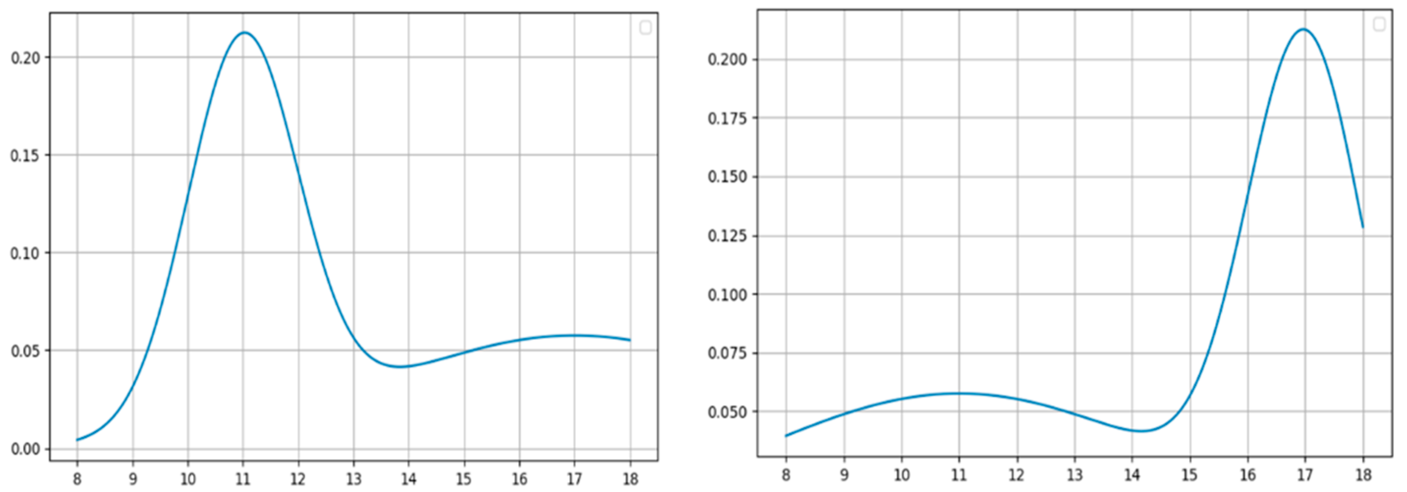
- Within each mini-depot’s service area, the demand time distribution of customer points is assumed to be known and predictable.
3.3. Model Establishment
3.3.1. Model Notation Definition
3.3.2. Clustering Stage
3.3.3. Optimizing Stage
4. Two-Stage Heuristic Algorithm
4.1. Clustering Stage: AP Clustering Algorithm
4.2. Optimizing Stage: Adaptive Heuristic Electric Eel Foraging Optimization
4.2.1. Algorithm Introduction
4.2.2. Fitness Function and Initial Solution
4.2.3. Algorithm Principle
- (1)
- Interacting behavior
- (2)
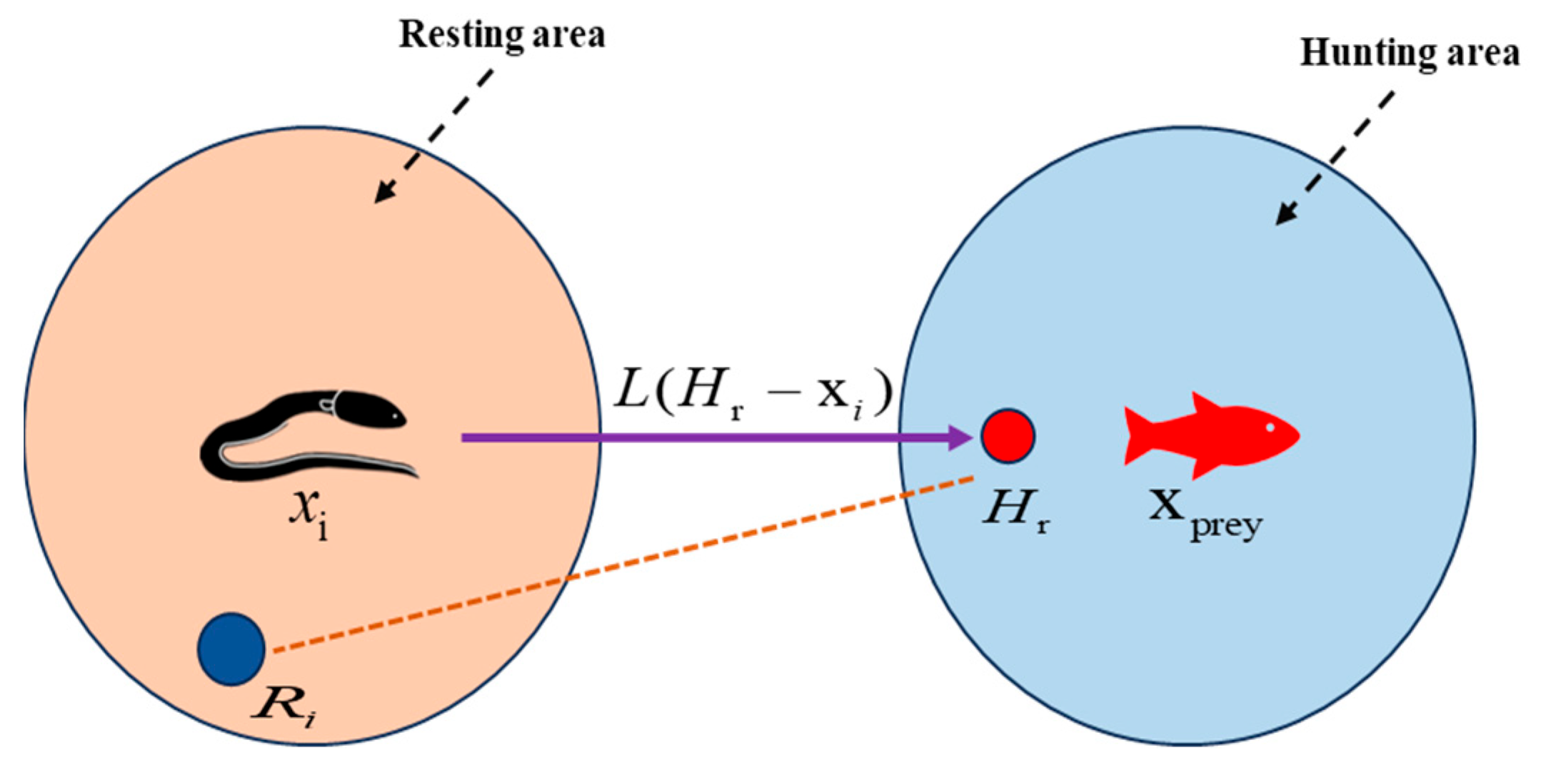
- Resting behavior
- (3)
- Hunting behavior
- (4)
- Migrating behavior
4.2.4. The Improvement Strategy of Limiting the Solution Space
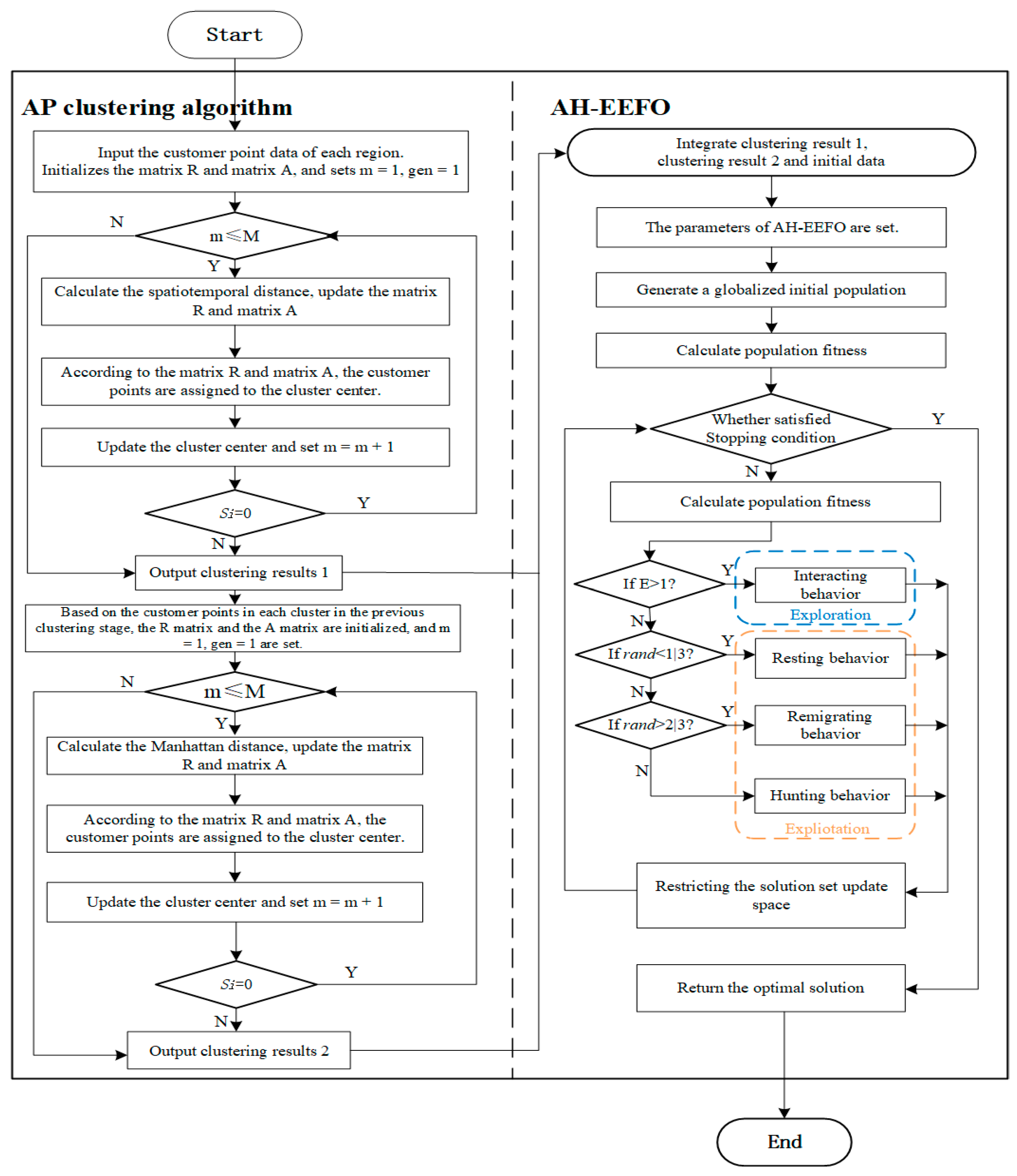
4.3. Two-Stage Heuristic Algorithm Procedure
| Algorithm 1 AHEEFO (Adaptive Heuristic Electric Eel Foraging Optimization) | |
| Input: Set parameters n and T. Randomly initialize the eel population Xi (i = 1,…,n), The population contains continuous variable part and discontinuous variable part (decision variable). And then evaluate their fitness Fiti, and Xprey is the best solution found so far. | |
| Output: The best solution Xprey | |
| 1 | while the stopping condition is not satisfied do |
| 2 | for each eel Xi do |
| 3 | Calculate E. |
| 4 | if E >1 |
| 5 | Perform the interacting behavior. |
| 6 | Evaluate the fitness Fiti. |
| 7 | Limit the update space of the current solution. |
| 8 | else |
| 9 | if rand > 1/3 |
| 10 | Determining the resting region. |
| 11 | Perform the resting behavior. |
| 12 | Evaluate the fitness Fiti. |
| 13 | Limit the update space of the current solution. |
| 14 | else If rand > 2/3 |
| 15 | Perform the migrating behavior. |
| 16 | Limit the update space of the current solution. |
| 17 | else |
| 18 | Determining the hunting region. |
| 19 | Perform the hunting behavior. |
| 20 | Limit the update space of the current solution. |
| 21 | end If |
| 22 | Update each eel’s position. |
| 23 | end For |
| 24 | Update the best solution found so far X |
| 25 | end While |
| 26 | return Xprey. |
5. Example Validation and Analysis
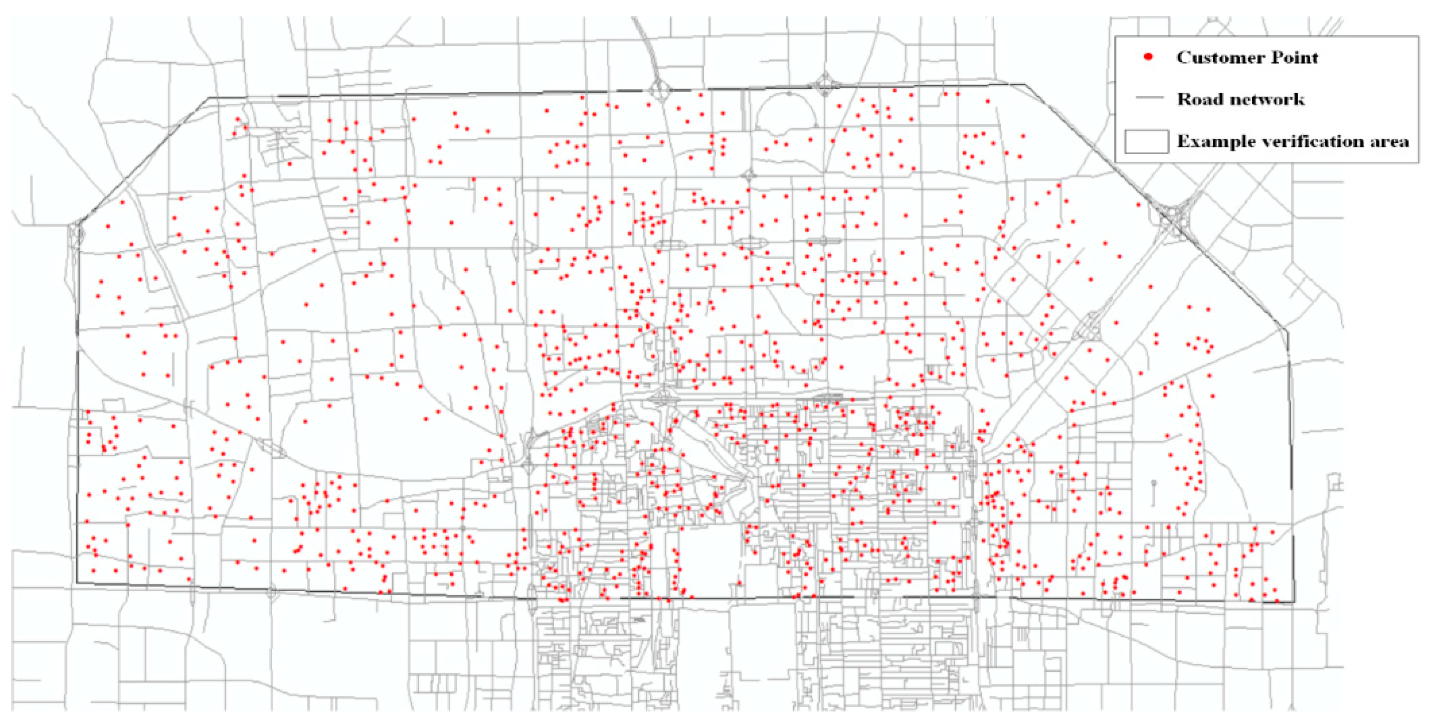
5.1. Generation of Problem Instances and Parameter Settings
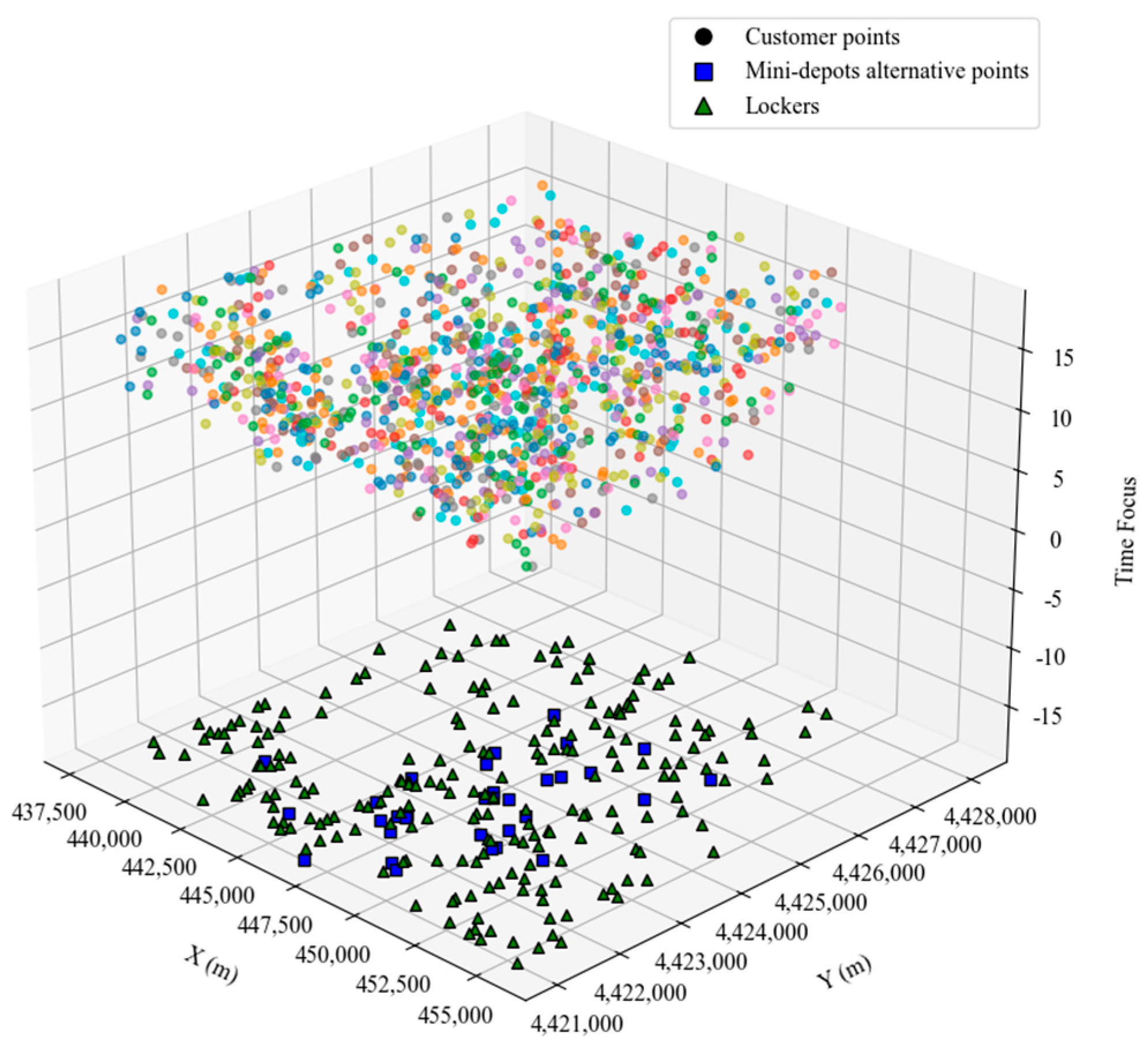
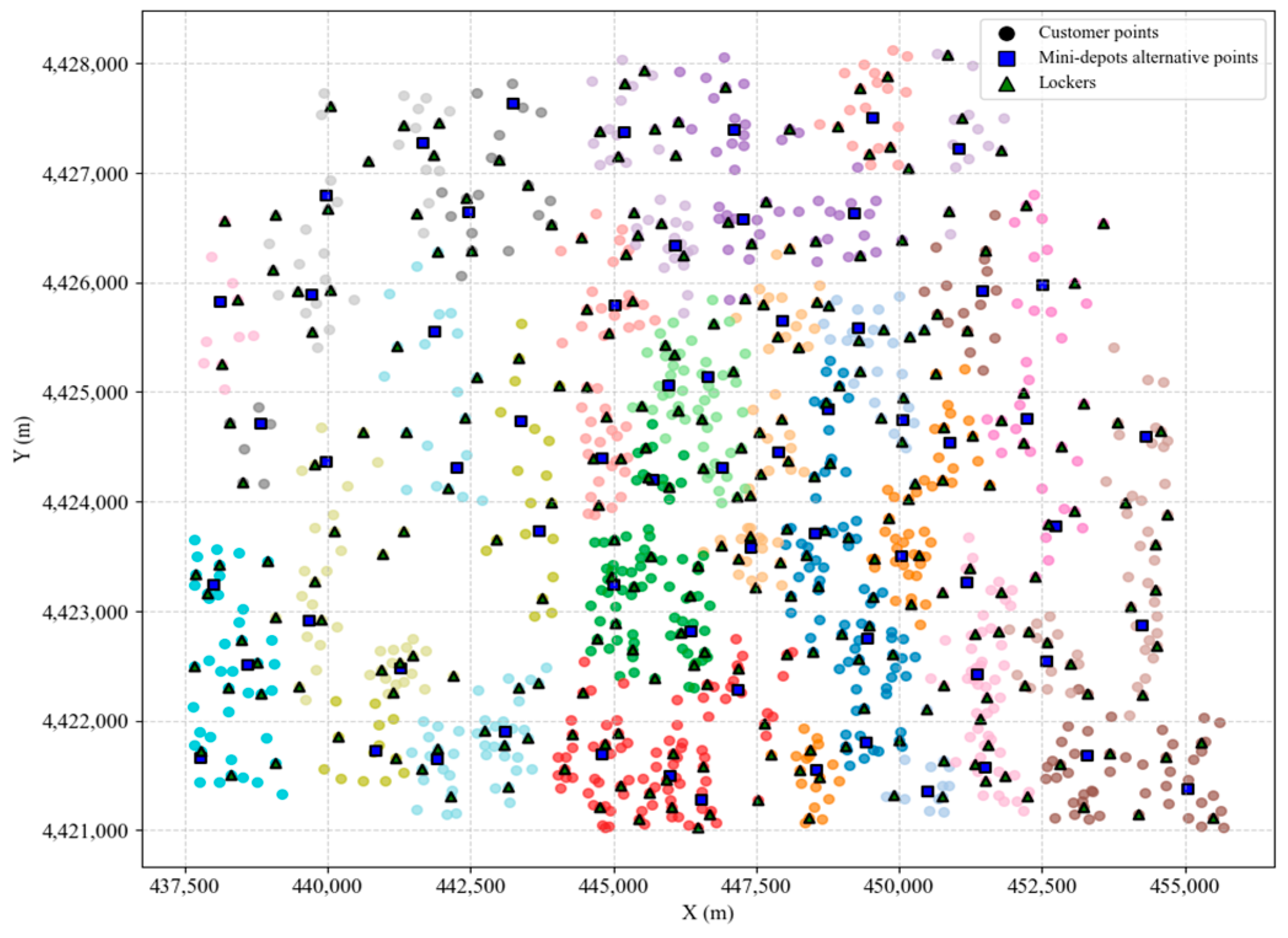
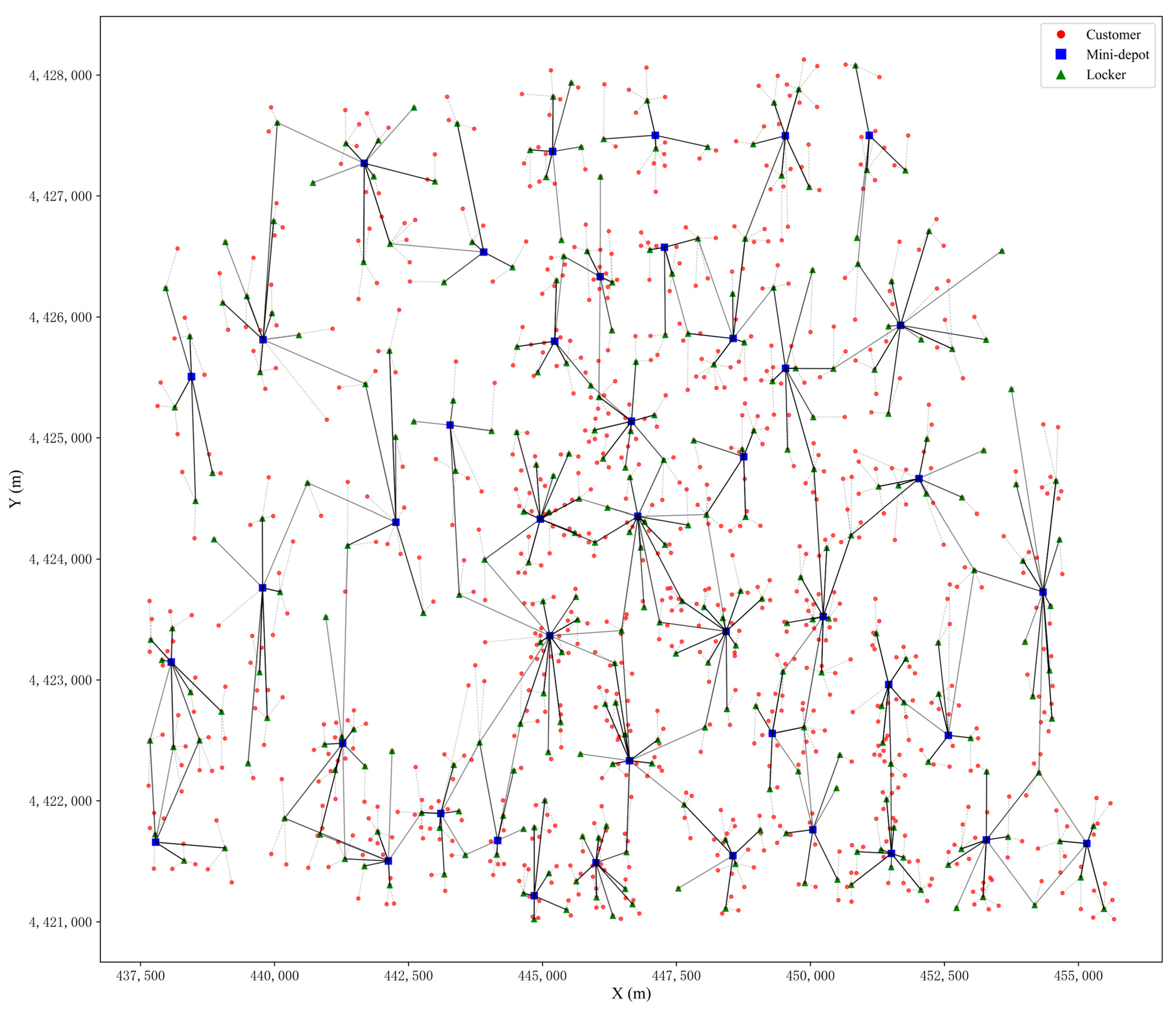
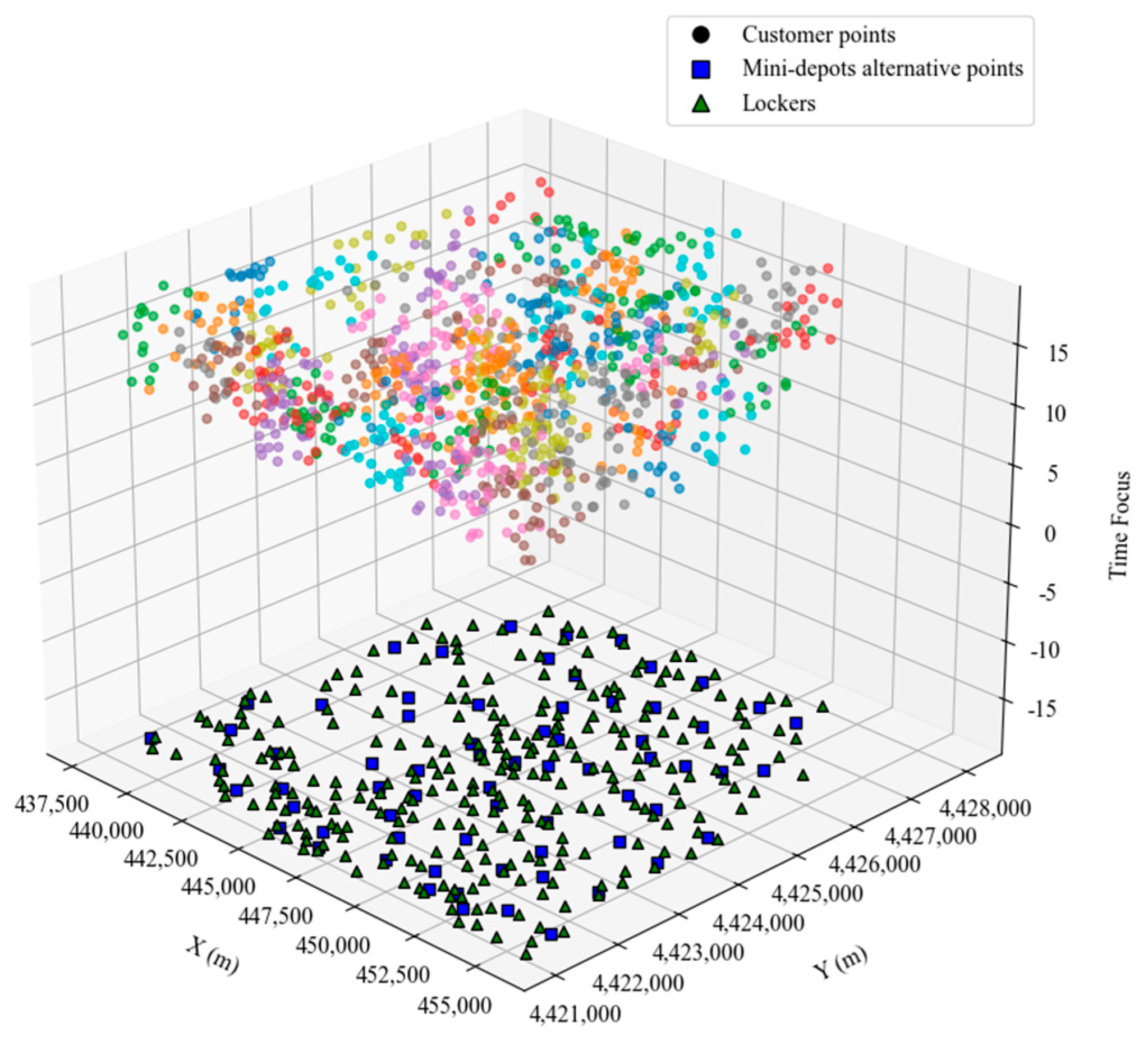
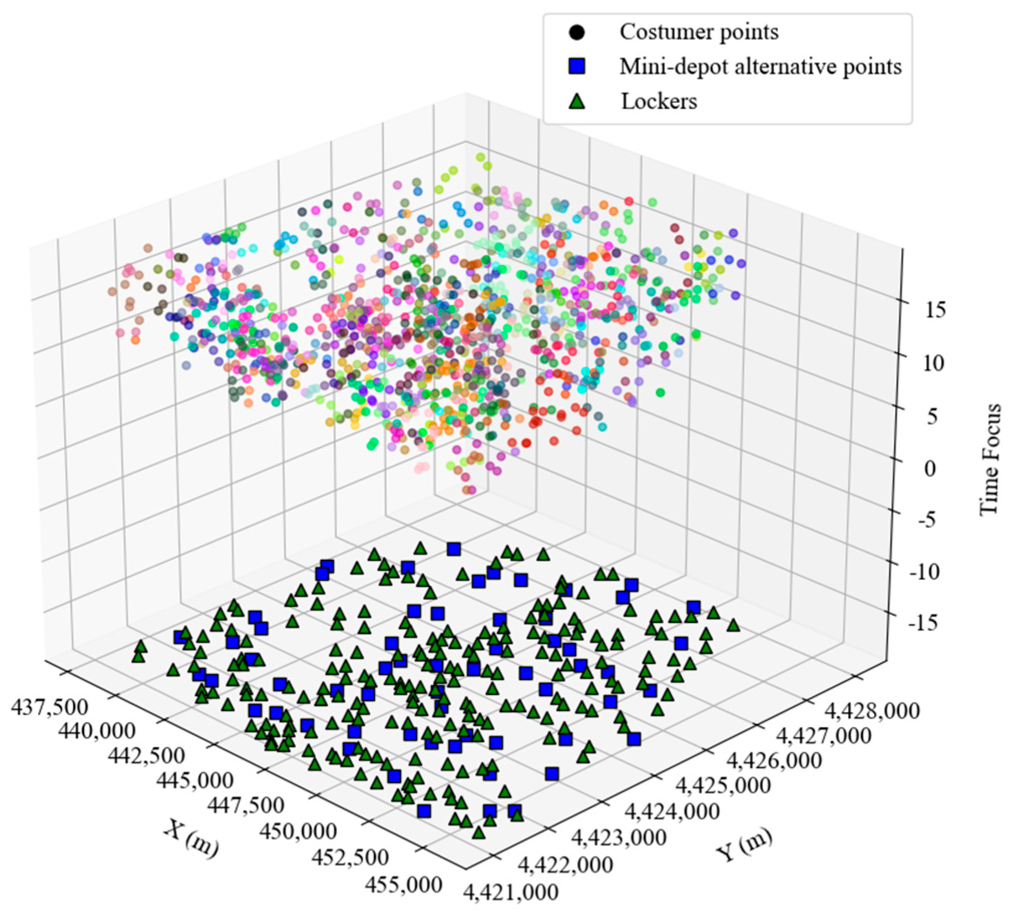
5.2. AP Clustering Selects the Location of Storage Lockers and Alternative Points
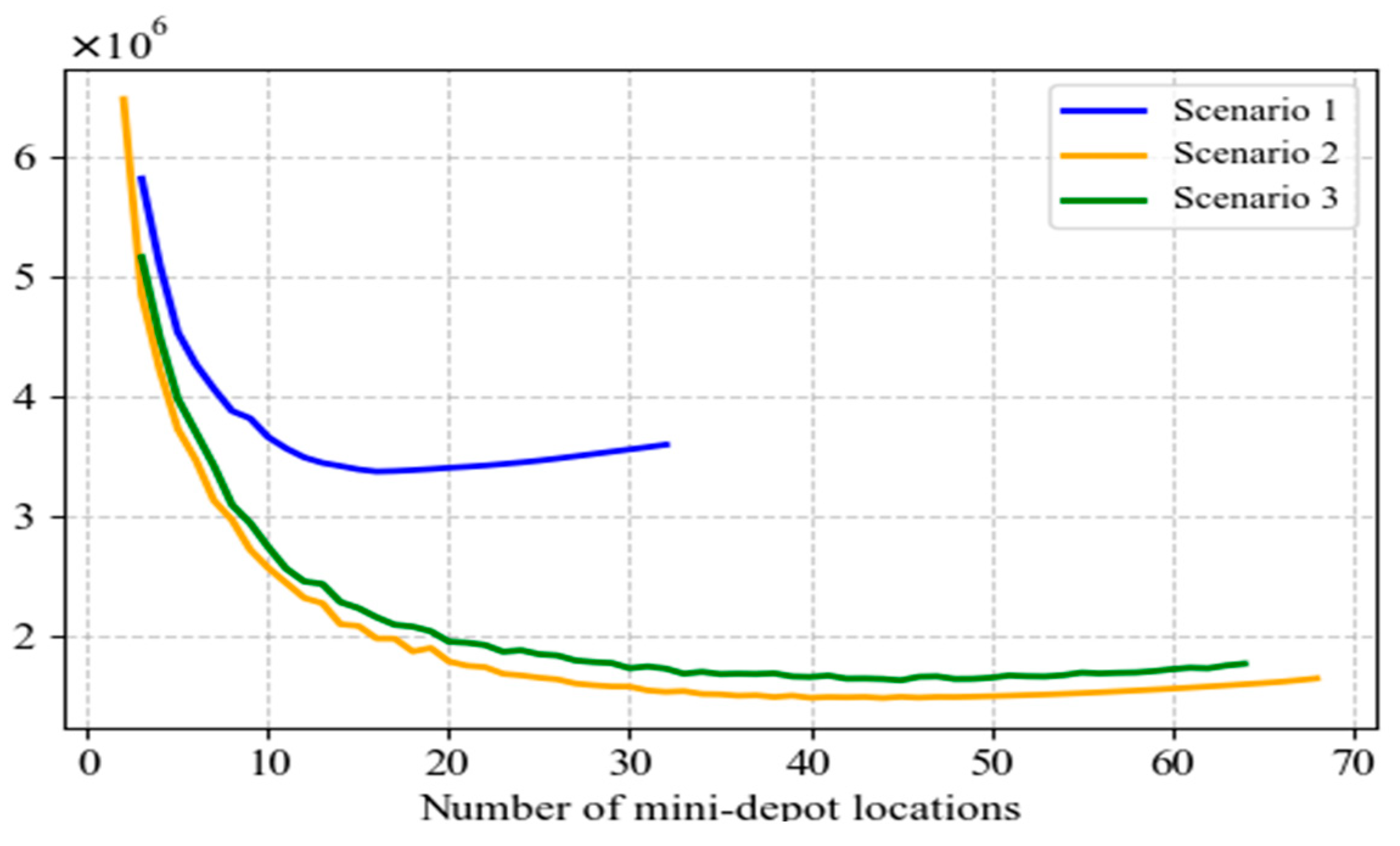
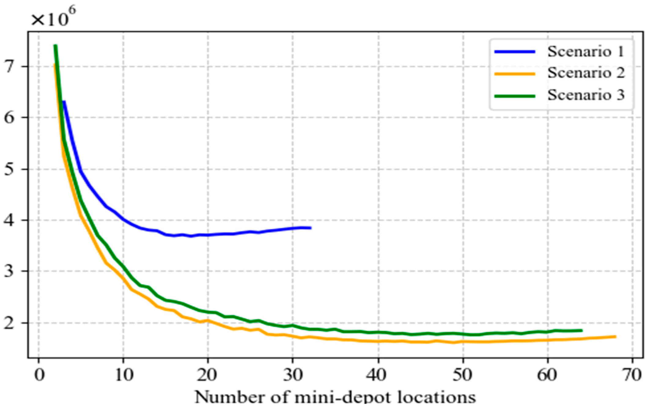
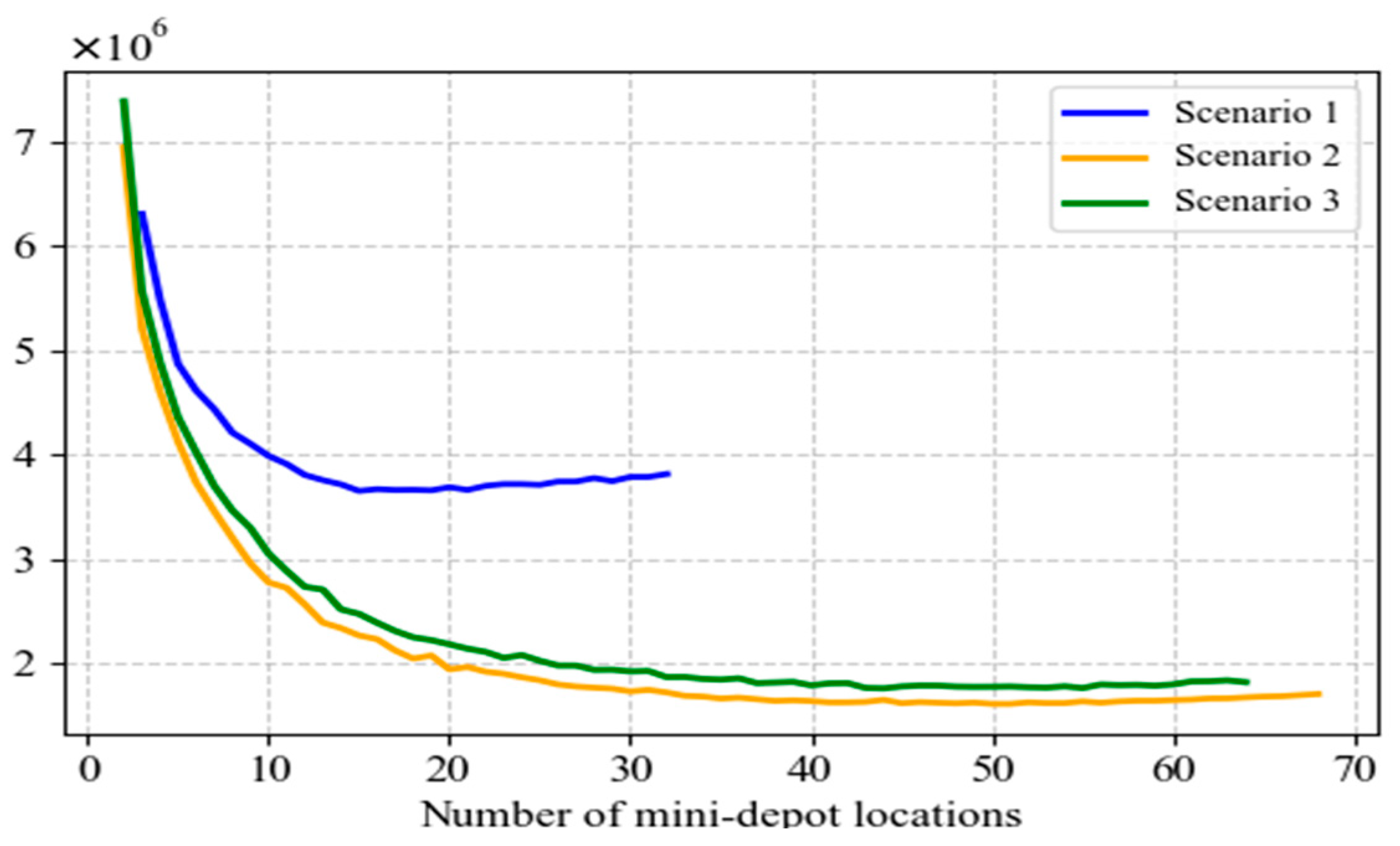
5.3. AHEEFO Solving Experimental Case
5.4. Algorithm Stability Experiment and Analysis
5.4.1. Stability Experiment and Analysis of AP Clustering
AP Clustering Validity and Stability Analysis
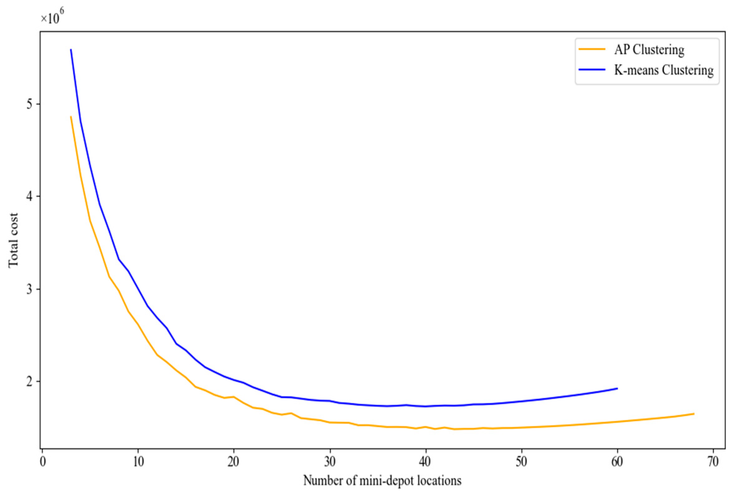
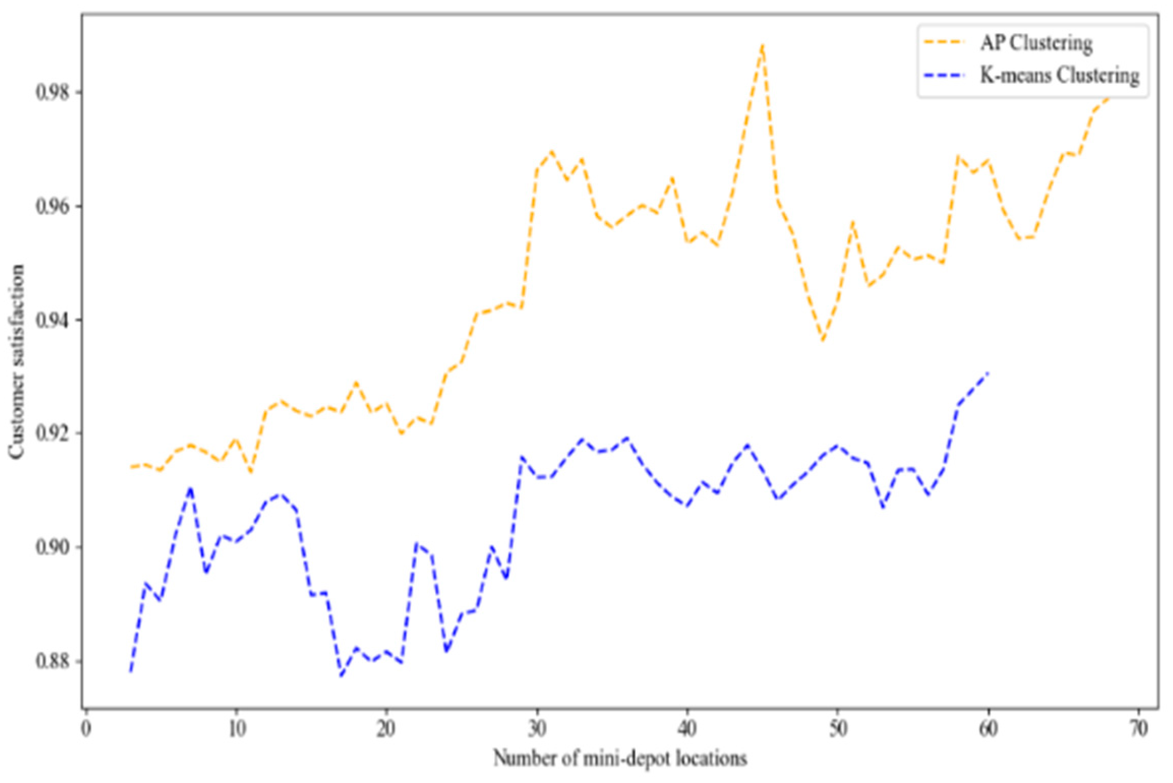
Comparison of the Effects of AP Clustering and K-Means Clustering on the Optimization Results Under Scenario 2
5.4.2. Stability Experiment and Analysis of AHEEFO
5.5. Sensitivity Analysis
6. Conclusions
- (1)
- Regardless of random surges in demand, the location strategy under Scenario 2 outperforms Scenario 1 and traditional location methods, achieving the lowest total cost and the highest customer satisfaction. This is because the dispersed temporal demand distribution allows crowd-sourced delivery to fully leverage its flexibility and cost advantages. By implementing elastic scheduling during peak periods and reasonably configuring lockers within service areas to share peak demand and shorten delivery distances, operational pressure is effectively alleviated while enhancing the customer experience. In contrast, Scenario 1’s concentrated demand pattern requires more professional courier resources during peak hours, leading to higher costs and limited efficiency.
- (2)
- The two-stage location model helps identify under which demand distribution scenarios crowd-sourced delivery is more appropriate than fixed-route delivery and provides decision support for the optimal configuration of lockers to relieve peak-period pressure. Policymakers can also draw on these findings to design more flexible incentive mechanisms for crowd-sourced riders or provide urban infrastructure support to optimize locker networks. Overall, the model integrates crowd-sourced delivery with locker deployment, providing e-commerce platforms with a sustainable “last mile” solution that balances cost control and high-quality service.
- (3)
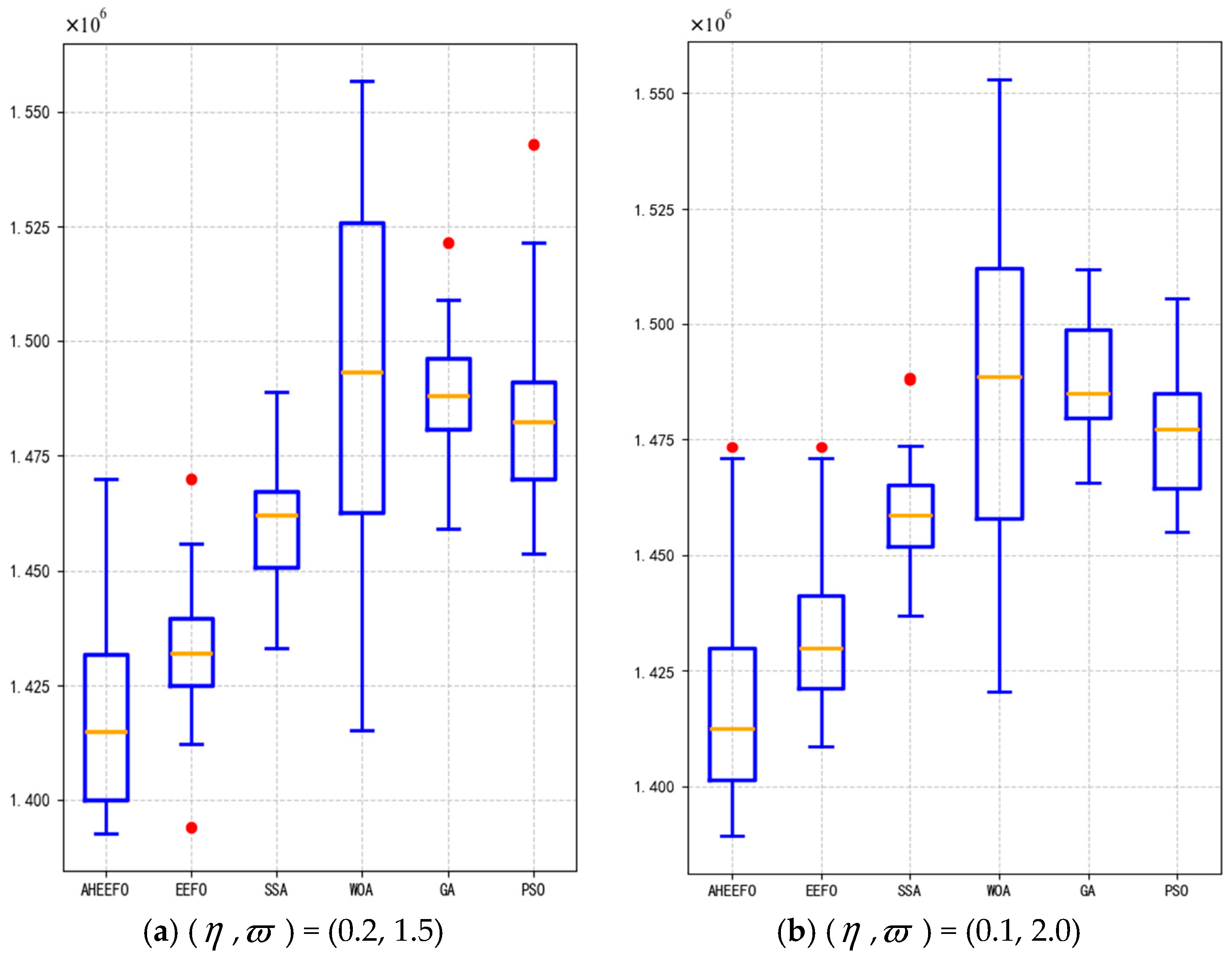
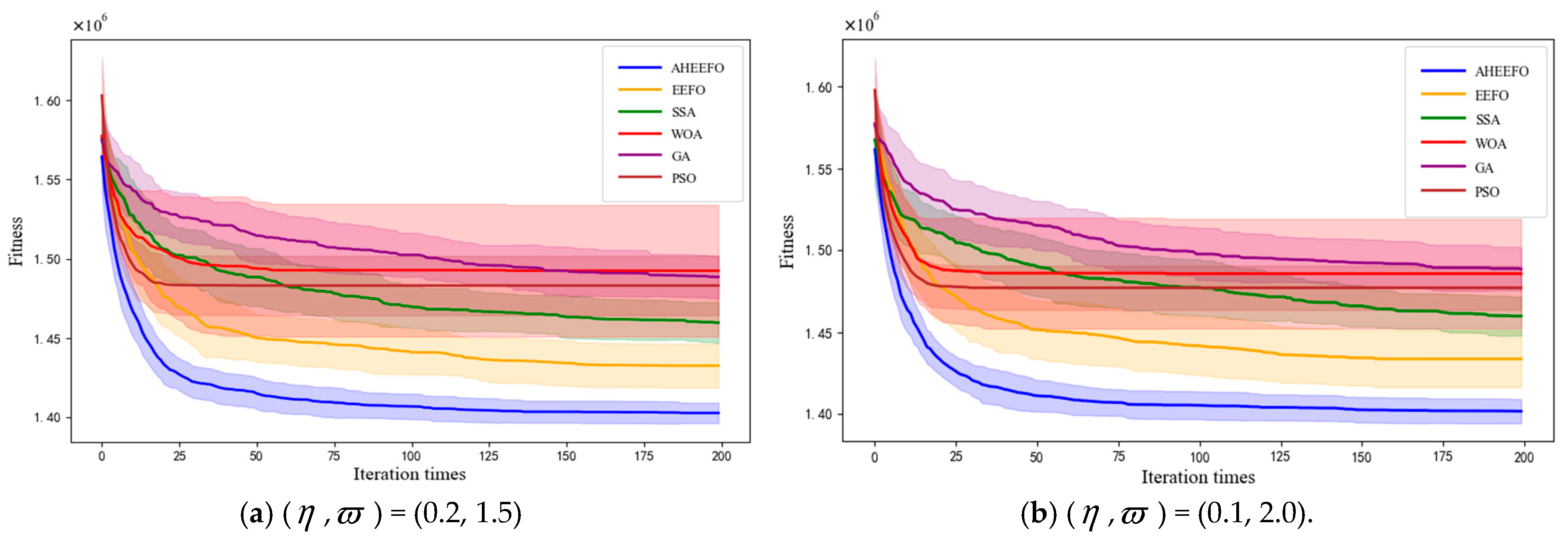
- The effectiveness of the proposed algorithm is verified through experimental cases. The results show that the model exhibits strong robustness under different random demand surges, with stable total cost and customer satisfaction. AP clustering demonstrates high compactness and separation, and maintains consistent clustering numbers and ARI values, indicating high reproducibility and providing more reliable input for subsequent location optimization. Compared with K-means, AP clustering reduces costs by 13.57% at the clustering stage. AHEEFO outperforms EEFO, SSA, WOA, GA, and PSO in terms of solution quality, computational efficiency, and stability.
- (4)
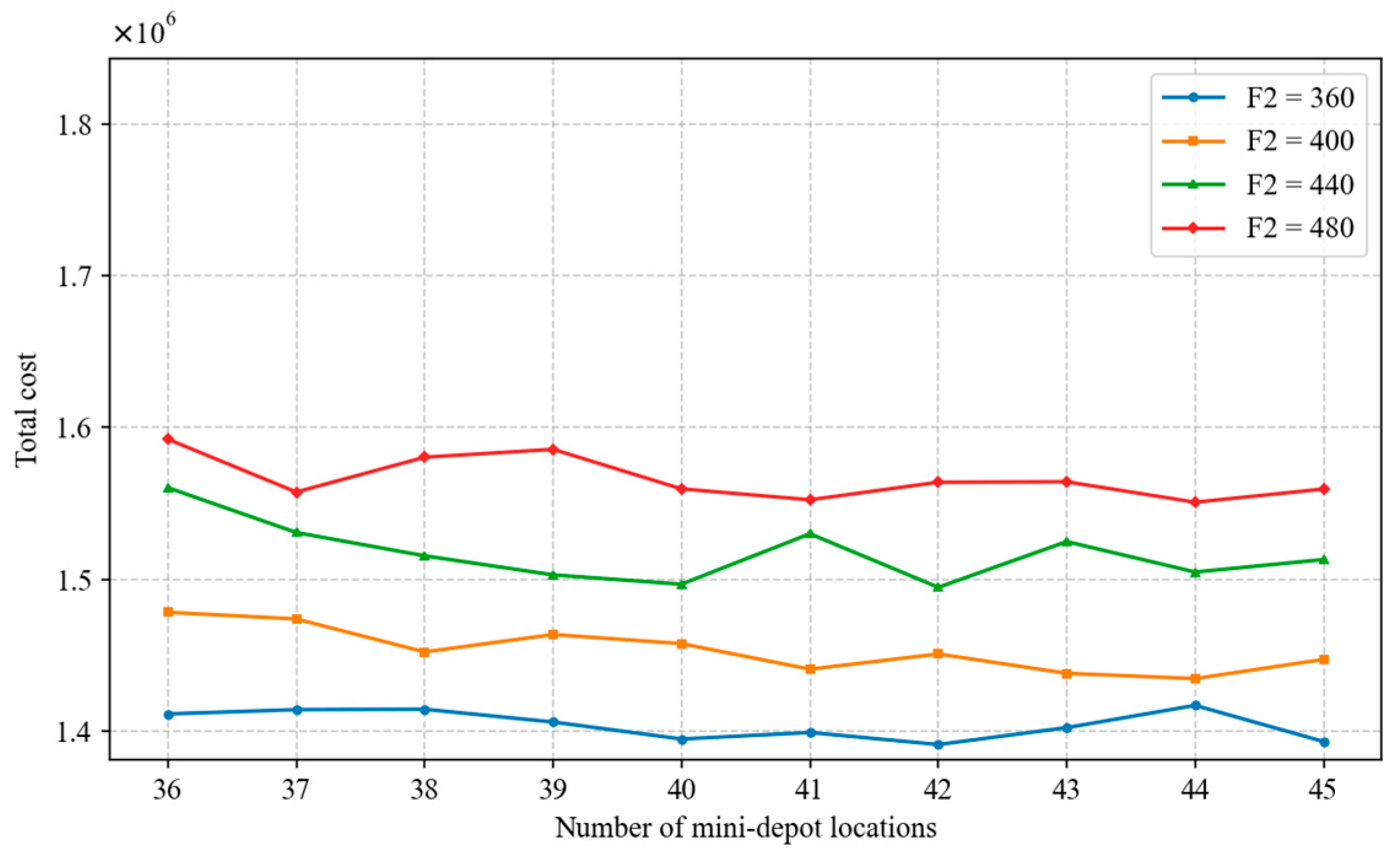
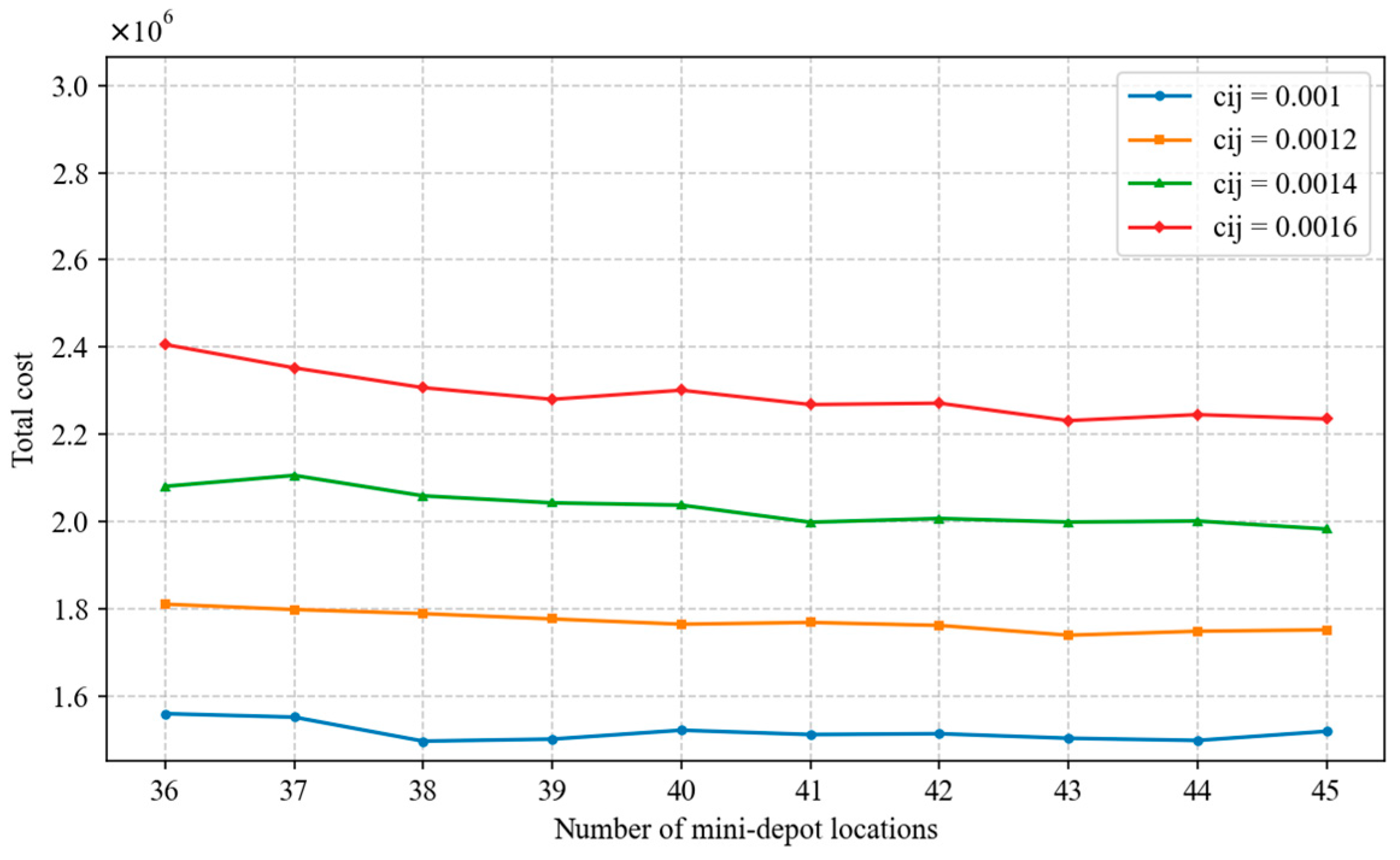
- The sensitivity analysis in this study indicates that when α = 20, the model achieves a good balance among facility location costs, delivery costs, and customer satisfaction. The algorithm parameter λ and operational parameter γ are the most sensitive factors affecting the location outcomes, whereas F2 and remain relatively stable. During the clustering stage for selecting candidate mini-depot sites and locker locations, setting λ to 0.7 helps achieve optimal location decisions, resulting in lower total costs. γ reflects customers’ sensitivity to delivery timeliness; therefore, firms should prioritize improving delivery performance through intelligent scheduling systems, rider route optimization, and instant delivery modes to reduce timeliness costs and enhance customer satisfaction. The analysis of F2 suggests that a moderate investment level (e.g., 400 yuan per month) is preferable, and firms should configure lockers considering both market rents and demand density. The stability of indicates that the overall layout remains robust even under fluctuations in fuel prices, electric vehicle electricity costs, or crowdsourcing commissions, providing firms with considerable flexibility in pricing changes. Overall, decision-makers should focus on the proper setting of λ and γ, while maintaining flexibility in investment and transportation cost management to address the dynamic demands of the e-commerce logistics industry.
Author Contributions
Funding
Institutional Review Board Statement
Informed Consent Statement
Data Availability Statement
Acknowledgments
Conflicts of Interest
References
- Sakai, T.; Santo, K.; Tanaka, S.; Hyodo, T. Locations of logistics facilities for e-commerce: A case of the Tokyo Metropolitan Area. Res. Transp. Bus. Manag. 2024, 56, 101174. [Google Scholar] [CrossRef]
- Heitz, A. The logistics dualization in question: Evidence from the Paris metropolitan area. Cities 2021, 119, 103407. [Google Scholar] [CrossRef]
- Aljohani, K.; Thompson, R.G. Impacts of logistics sprawl on the urban environment and logistics: Taxonomy and review of literature. J. Transp. Geogr. 2016, 57, 255–263. [Google Scholar] [CrossRef]
- He, M.; Shen, J.; Wu, X.; Luo, J. Logistics Space: A Literature Review from the Sustainability Perspective. Sustainability 2018, 10, 2815. [Google Scholar] [CrossRef]
- Zhang, R.; Liu, H.; Xie, K.; Xiao, W.; Bai, C. Toward a low carbon path: Do E-commerce reduce CO2 emissions? Evidence from China. J. Environ. Manag. 2024, 351, 119805. [Google Scholar] [CrossRef]
- Hu, S.; Zhang, H.; Wang, Y. Does e-commerce development drive regional entrepreneurial activity? Spatial spillover effect and mechanism analysis. Int. J. Prod. Econ. 2025, 284, 109611. [Google Scholar] [CrossRef]
- Beckers, J.; Cardenas, I.; Sanchez-Diaz, I. Managing household freight: The impact of online shopping on residential freight trips. Transp. Policy 2022, 125, 299–311. [Google Scholar] [CrossRef]
- Kang, S. Relative logistics sprawl: Measuring changes in the relative distribution from warehouses to logistics businesses and the general population. J. Transp. Geogr. 2020, 83, 102636. [Google Scholar] [CrossRef]
- Rai, J.K. Creating the Discourse of Marginalized Limbu Community: A Foucauldian Analysis of Manglak’s Limbuni Gaaun [The Village of Limbu Woman]. JODEM J. Lang. Lit. 2022, 13, 41–52. [Google Scholar] [CrossRef]
- Jaller, M.; Otero-Palencia, C.; Pahwa, A. Automation, electrification, and shared mobility in urban freight: Opportunities and challenges. Transp. Res. Procedia 2020, 46, 13–20. [Google Scholar] [CrossRef]
- Steins, J.J.; Ruck, M.; Volk, R.; Schultmann, F. Optimal design of a post-demolition autoclaved aerated concrete (AAC) recycling network using a capacitated, multi-period, and multi-stage warehouse location problem. J. Clean. Prod. 2024, 474, 143580. [Google Scholar] [CrossRef]
- Shahparvari, S.; Nasirian, A.; Mohammadi, A.; Noori, S.; Chhetri, P. A GIS-LP integrated approach for the logistics hub location problem. Comput. Ind. Eng. 2020, 146, 106488. [Google Scholar] [CrossRef]
- Lu, F.; Jiang, R.; Bi, H.; Gao, Z. Order Distribution and Routing Optimization for Takeout Delivery under Drone–Rider Joint Delivery Mode. J. Theor. Appl. Electron. Commer. Res. 2024, 19, 774–796. [Google Scholar] [CrossRef]
- Wang, Y.; Gou, M.; Luo, S.; Fan, J.; Wang, H. The multi-depot pickup and delivery vehicle routing problem with time windows and dynamic demands. Eng. Appl. Artif. Intell. 2025, 139, 109700. [Google Scholar] [CrossRef]
- Nasr, N.; Niaki, S.T.A.; Hussenzadek Kashan, A.; Seifbarghy, M. An efficient solution method for an agri-fresh food supply chain: Hybridization of Lagrangian relaxation and genetic algorithm. Environ. Sci. Pollut. Res. Int. 2021, 1–19. [Google Scholar] [CrossRef]
- Kahalimoghadam, M.; Thompson, R.G.; Rajabifard, A. Determining the number and location of micro-consolidation centres as a solution to growing e-commerce demand. J. Transp. Geogr. 2024, 117, 103875. [Google Scholar] [CrossRef]
- Savchenko, L.; Grygorak, M.; Polishchuk, V.; Vovk, Y.; Lyashuk, O.; Vovk, I.; Khudobei, R. Complex Evaluation of the Efficiency of Urban Consolidation Centers at the Micro Level. Sci. J. Silesian Univ. Technol. Ser. Transp. 2022, 115, 135–159. [Google Scholar] [CrossRef]
- Nieto-Isaza, S.; Fontaine, P.; Minner, S. The value of stochastic crowd resources and strategic location of mini-depots for last-mile delivery: A Benders decomposition approach. Transp. Res. Part B Methodol. 2022, 157, 62–79. [Google Scholar] [CrossRef]
- Bi, H.; Gu, Y.; Lu, F.; Mahreen, S. Site selection of electric vehicle charging station expansion based on GIS-FAHP-MABAC. J. Clean. Prod. 2025, 507, 145557. [Google Scholar] [CrossRef]
- Kundu, T.; Goh, M.; Choi, T. Home delivery vs. out-of-home delivery: Syncretic value-based strategies for urban last-mile e-commerce logistics. Transp. Res. Part A Policy Pract. 2025, 193, 104309. [Google Scholar] [CrossRef]
- Chen, L.; Han, S.; Ye, Z.; Xia, S. The optimisation of the location of front distribution centre: A spatio-temporal joint perspective. Int. J. Prod. Econ. 2023, 263, 108950. [Google Scholar] [CrossRef]
- Zhao, W.; Wang, L.; Zhang, Z.; Fan, H.; Zhang, J.; Mirjalili, S.; Khodadadi, N.; Cao, Q. Electric eel foraging optimization: A new bio-inspired optimizer for engineering applications. Expert Syst. Appl. 2024, 238, 122200. [Google Scholar] [CrossRef]
- Liu, S.; He, L.; Max Shen, Z. On-time last-mile delivery: Order assignment with travel-time predictors. Manag. Sci. 2021, 67, 4095–4119. [Google Scholar] [CrossRef]
- Gdowska, K.; Viana, A.; Pedroso, J.P. Stochastic last-mile delivery with crowdshipping. Transp. Res. Procedia 2018, 30, 90–100. [Google Scholar] [CrossRef]
- Deng, Q.; Fang, X.; Lim, Y.F. Urban Consolidation Center or Peer-to-Peer Platform? The Solution to Urban Last-Mile Delivery. Prod. Oper. Manag. 2021, 30, 997–1013. [Google Scholar] [CrossRef]
- Mousavi, K.; Bodur, M.; Roorda, M.J. Stochastic last-mile delivery with crowd-shipping and mobile depots. Transp. Sci. 2022, 56, 612–630. [Google Scholar] [CrossRef]
- Pourrahmani, E.; Jaller, M. Crowdshipping in last mile deliveries: Operational challenges and research opportunities. Socio-Econ. Plan. Sci. 2021, 78, 101063. [Google Scholar] [CrossRef]
- Lu, F.; Du, Z.; Wang, Z.; Wang, L.; Wang, S. Towards enhancing the crowdsourcing door-to-door delivery: An effective model in Beijing. J. Ind. Manag. Optim 2025, 21, 2371–2395. [Google Scholar] [CrossRef]
- Tao, Y.; Zhuo, H.; Lai, X. The pickup and delivery problem with multiple depots and dynamic occasional drivers in crowdshipping delivery. Comput. Ind. Eng. 2023, 182, 109440. [Google Scholar] [CrossRef]
- Tapia, R.J.; Kourounioti, I.; Thoen, S.; de Bok, M.; Tavasszy, L. A disaggregate model of passenger-freight matching in crowdshipping services. Transp. Res. Part A Policy Pract. 2023, 169, 103587. [Google Scholar] [CrossRef]
- Nsamzinshuti, A.; Cardoso, F.; Janjevic, M.; Ndiaye, A.B. Pharmaceutical distribution in urban area: An integrated analysis and perspective of the case of Brussels-Capital Region (BRC). Transp. Res. Procedia 2017, 25, 747–761. [Google Scholar] [CrossRef]
- Oliveira, L.K.; Oliveira, I.K.; Nascimento, C.D.O.L.; Marcucci, E.; Gatta, V. Mobility as a service for freight and passenger transport: Identifying a microhubs network to promote crowdshipping service. Case Stud. Transp. Policy 2025, 19, 101356. [Google Scholar] [CrossRef]
- Lin, Y.H.; Wang, Y.; He, D.; Lee, L.H. Last-mile delivery: Optimal locker location under multinomial logit choice model. Transp. Res. Part E Logist. Transp. Rev. 2020, 142, 102059. [Google Scholar] [CrossRef]
- Deutsch, Y.; Golany, B. A parcel locker network as a solution to the logistics last mile problem. Int. J. Prod. Res. 2018, 56, 251–261. [Google Scholar] [CrossRef]
- Faugère, L.; Montreuil, B. Smart locker bank design optimization for urban omnichannel logistics: Assessing monolithic vs. modular configurations. Comput. Ind. Eng. 2020, 139, 105544. [Google Scholar] [CrossRef]
- Ghaderi, H.; Zhang, L.; Tsai, P.; Woo, J. Crowdsourced last-mile delivery with parcel lockers. Int. J. Prod. Econ. 2022, 251, 108549. [Google Scholar] [CrossRef]
- Raviv, T. The service points’ location and capacity problem. Transp. Res. Part E Logist. Transp. Rev. 2023, 176, 103216. [Google Scholar] [CrossRef]
- Wang, L.; Xu, M.; Qin, H. Joint optimization of parcel allocation and crowd routing for crowdsourced last-mile delivery. Transp. Res. Part B Methodol. 2023, 171, 111–135. [Google Scholar] [CrossRef]
- Boysen, N.; de Koster, R.; Weidinger, F. Warehousing in the e-commerce era: A survey. Eur. J. Oper. Res. 2019, 277, 396–411. [Google Scholar] [CrossRef]
- Xiao, Z.; Yuan, Q.; Sun, Y.; Sun, X. New paradigm of logistics space reorganization: E-commerce, land use, and supply chain management. Transp. Res. Interdiscip. Perspect. 2021, 9, 100300. [Google Scholar] [CrossRef]
- Lozzi, R.; Marcucci, E.; Gatta, V. Urban logistics facilities and storytelling. Stakeholder engagement, participatory policy-planning and co-creation. Transp. Plan. Technol 2025, 1–23. [Google Scholar] [CrossRef]
- Kovač, M.; Tadić, S.; Krstić, M.; Bouraima, M.B. Novel Spherical Fuzzy MARCOS Method for Assessment of Drone-Based City Logistics Concepts. Complexity 2021, 2021, 2374955. [Google Scholar] [CrossRef]
- Rudolph, C.; Nsamzinshuti, A.; Bonsu, S.; Ndiaye, A.B.; Rigo, N. Localization of relevant urban micro-consolidation centers for last-mile cargo bike delivery based on real demand data and city characteristics. Transp. Res. Rec. 2022, 2676, 365–375. [Google Scholar] [CrossRef]
- Arrieta Prieto, M.; Ismael, A.; Rivera Gonzalez, C.; Mitchell, J.E. Location of urban micro-consolidation centers to reduce the social cost of last-mile deliveries of cargo: A heuristic approach. Networks 2022, 79, 292–313. [Google Scholar] [CrossRef]
- Tadić, S.; Krstić, M.; Kovač, M.; Brnjac, N. Evaluation of smart city logistics solutions. Promet-TrafficTransportation 2022, 34, 725–738. [Google Scholar] [CrossRef]
- Yazdekhasti, A.; Ma, J. A two-echelon two-indenture warranty distribution network development and optimization under batch-ordering inventory policy. Int. J. Prod. Econ. 2022, 249, 108508. [Google Scholar] [CrossRef]
- Zhou, J.; Yang, C.; Liu, D.; Wang, Y.; Zhong, Z.; Wu, Y. A three-stage geospatial network optimal location decision model for urban green logistics centers from a sustainable perspective. Sustain. Cities Soc. 2025, 128, 106481. [Google Scholar] [CrossRef]
- Rajendran, S.; Zack, J. Insights on strategic air taxi network infrastructure locations using an iterative constrained clustering approach. Transp. Res. Part E Logist. Transp. Rev. 2019, 128, 470–505. [Google Scholar] [CrossRef]
- Lei, G.; Baina, H.; Jingru, Z.; Chenxu, L.; Zuyuan, L.; Weihan, D.; Ye, L.; Moqian, W. Location and sizing of distributed energy storage in distribution substations under multiple scenarios based on improved affinity propagation clustering. Electr. Power Syst. Res. 2025, 248, 111898. [Google Scholar] [CrossRef]
- Fan, H.; Zhang, Y.; Tian, P.; Lv, Y.; Fan, H. Time-dependent multi-depot green vehicle routing problem with time windows considering temporal-spatial distance. Comput. Oper. Res. 2021, 129, 105211. [Google Scholar] [CrossRef]
- Esmaeilnejad, S.; Kattan, L.; Wirasinghe, S.C. Optimal charging station locations and durations for a transit route with battery-electric buses: A two-stage stochastic programming approach with consideration of weather conditions. Transp. Res. Part C Emerg. Technol. 2023, 156, 104327. [Google Scholar] [CrossRef]
- Aghalari, A.; Salamah, D.; Kabli, M.; Marufuzzaman, M. A two-stage stochastic location–routing problem for electric vehicles fast charging. Comput. Oper. Res. 2023, 158, 106286. [Google Scholar] [CrossRef]
- Nascimento, C.D.O.L.; Gatta, V.; Marcucci, E. Green Crowdshipping: Critical factors from a business perspective. Res. Transp. Bus. Manag. 2023, 51, 101062. [Google Scholar] [CrossRef]
- Guidotti, R.; Gabrielli, L.; Monreale, A.; Pedreschi, D.; Giannotti, F. Discovering temporal regularities in retail customers’ shopping behavior. EPJ Data Sci. 2018, 7, 6. [Google Scholar] [CrossRef]
- Wu, Y.; Geunes, J.; Nie, X. Revisiting Continuous p-Hub Location Problems with the L1 Metric. arXiv 2025, arXiv:2501.08439. [Google Scholar] [CrossRef]
- Brimberg, J.; Hansen, P.; Mladenović, N.; Taillard, E.D. Improvements and comparison of heuristics for solving the uncapacitated multisource Weber problem. Oper. Res. 2000, 48, 444–460. [Google Scholar] [CrossRef]
- Farahani, R.Z.; SteadieSeifi, M.; Asgari, N. Multiple criteria facility location problems: A survey. Appl. Math. Model. 2010, 34, 1689–1709. [Google Scholar] [CrossRef]
- Ma, Y.F.; Yang, C.; Zhang, M.; Hao, C. Time-satisfaction-based maximal covering location problem. Chin. J. Manag. Sci. 2006, 14, 45–51. [Google Scholar]
- Lu, F.; Gao, Z.; Jiang, R.; Bi, H. Routing Optimization of Takeout Delivery Routes Under Joint Delivery Model of Drones, Occasional Drivers, and Riders. IEEE Trans. Intell. Transp. Syst. 2025, 1–10. [Google Scholar] [CrossRef]
- Lin, Y.; Wang, Y.; Lee, L.H.; Chew, E.P. Profit-maximizing parcel locker location problem under threshold Luce model. Transp. Res. Part E Logist. Transp. Rev. 2022, 157, 102541. [Google Scholar] [CrossRef]
- Liu, Y.; Ye, Q.; Escribano-Macias, J.; Feng, Y.; Candela, E.; Angeloudis, P. Route planning for last-mile deliveries using mobile parcel lockers: A hybrid q-learning network approach. Transp. Res. Part E Logist. Transp. Rev. 2023, 177, 103234. [Google Scholar] [CrossRef]
- Lu, F.; Meng, F.; Bi, H. Scenario deduction of explosion accident based on fuzzy dynamic Bayesian network. J. Loss Prev. Process Ind. 2025, 96, 105613. [Google Scholar] [CrossRef]
- Lu, F.; Gao, Z.; Bi, H. Bi-objective green vehicle routing problem with heterogeneous regular vehicles and occasional drivers joint delivery. Comput. Manag. Sci. 2025, 22, 18. [Google Scholar] [CrossRef]






| Reference | Findings | Consideration Factors | ||
|---|---|---|---|---|
| Distribution Cost | Customer Satisfaction | Env. Cost | ||
| [18] | On the network based on the Munich public transport network, mini-depots combined with random crowdsourcing resources can improve distribution efficiency and reduce distribution costs. | √ | × | × |
| [31] | In the Brussels-Capital Region, MCCs can significantly reduce wholesale distributor transportation costs and congestion. | √ | × | √ |
| [42] | The most effective concept for improving LMD efficiency is a two-echelon system with MCCs. | × | × | √ |
| [17] | MCCs were more socioeconomically advantageous than direct delivery in Poznan. | √ | × | × |
| [43] | In Stuttgart, MCCs have been used to facilitate the use of environmentally friendly vehicles. | √ | × | × |
| [44] | The implementation of MCCs in Manhattan resulted in reduced service time and pollution, as indicated by simulation results. | × | × | √ |
| [45] | The reduction in adverse effects of goods movement was addressed by the combination of MCCs and autonomous vehicles in the LMD. | × | × | √ |
| [16] | MCCs are set up in the city of Sydney, Australia to provide services for PLs, to establish a collaborative LMD network, and ultimately by the customer to the parcel cabinet to pick up the package. The results show that because MCC is close to the final distribution location, the distribution cost can be significantly reduced. | √ | × | √ |
| Stage | Type | Symbol | Definition |
|---|---|---|---|
| Clustering stage | parameters | x-coordinate of customer point j. | |
| y-coordinate of customer point j. | |||
| Coefficient that controls the demand time distribution function. | |||
| and | Independent mean in the demand time distribution function. | ||
| and | Independent standard deviation in the demand time distribution function. | ||
| The damping factor, and λ ∈ [0, 1]. | |||
| Spatio-temporal coefficient that controls the influence degree from space and time dimensions, and β ∈ [0, 1]. | |||
| Optimizing stage | parameters | I | Set of alternative points, I = {1, 2, 3,…, k1}, where k1 is the total number of alternative points determined by AP clustering. |
| i | Alternative points index, and i ∈ I. | ||
| J | Set of customer demand points, J = {1, 2, 3,…, n1}, where n1 is the total number of customer demand points. | ||
| j | Customer demand points index, and j ∈ J. | ||
| M | Set of lockers, M = {1, 2, 3,…, k2}, where k2 is the total number of lockers determined by AP clustering. | ||
| m | Lockers index, and m ∈ M. | ||
| N | Set of crowdsourcing destinations, N = {1, 2, 3,…, n2}, where n2 is the total number of crowdsourcing destinations. | ||
| n | Crowdsourcing destinations index, and n ∈ N. | ||
| another variable sets and indices | C1 | Fixed investment cost. | |
| C2 | Parcel transportation cost. | ||
| wj | Parcel demands of Customer demand point j. | ||
| dij | Delivery distance from mini-depot i to customer demand point j. | ||
| dim | Delivery distance from mini-depot i to locker m. | ||
| dmj | The distance from intelligent locker m to customer demand point j. | ||
| Unit transportation rate from alternative point i to customer demand point j. | |||
| F1 | Fixed rental cost of each mini-depot. | ||
| F2 | Fixed rental cost each locker. | ||
| r | The cost of unit power consumption of battery car. | ||
| e | Units outside the crowdsourcing service distance compensate for the delivery cost. | ||
| Q | Lockers’ capacity. | ||
| v | Average delivery speed of crowdsourcing distributors. | ||
| Demand surge probability. | |||
| Demand surge multiples | |||
| Ω | Crowdsourcing distributor distribution range coefficient. | ||
| α | Cost-satisfaction trade-off coefficient | ||
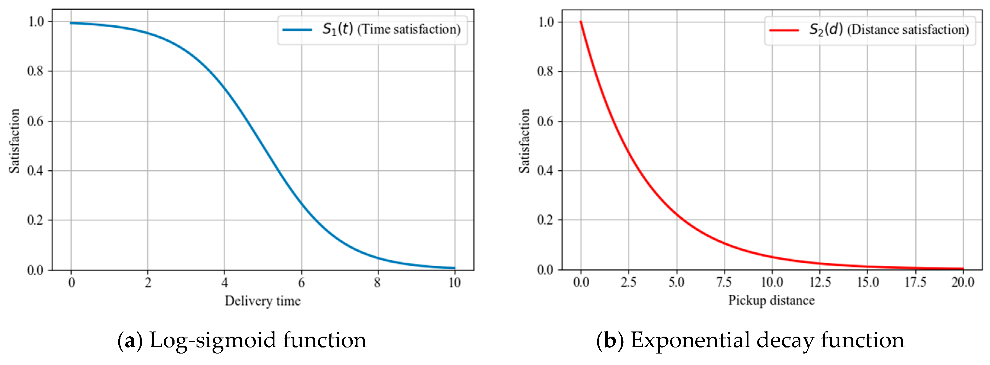
| γ | Positive time sensitivity coefficient of customer satisfaction in door-to-door delivery service. | ||
| θ | Decay constant. | ||
| tij | Delivery time from mini-depot i to customer demand point j. | ||
| Lj | The longest waiting time accepted by customer demand point j. | ||
| D1 | Mini-depot maximum service distance. | ||
| D2 | The preferred self-pickup distance | ||
| Rmin | Minimum service radius of locker. | ||
| Rmax | Maximum service radius of lockers. | ||
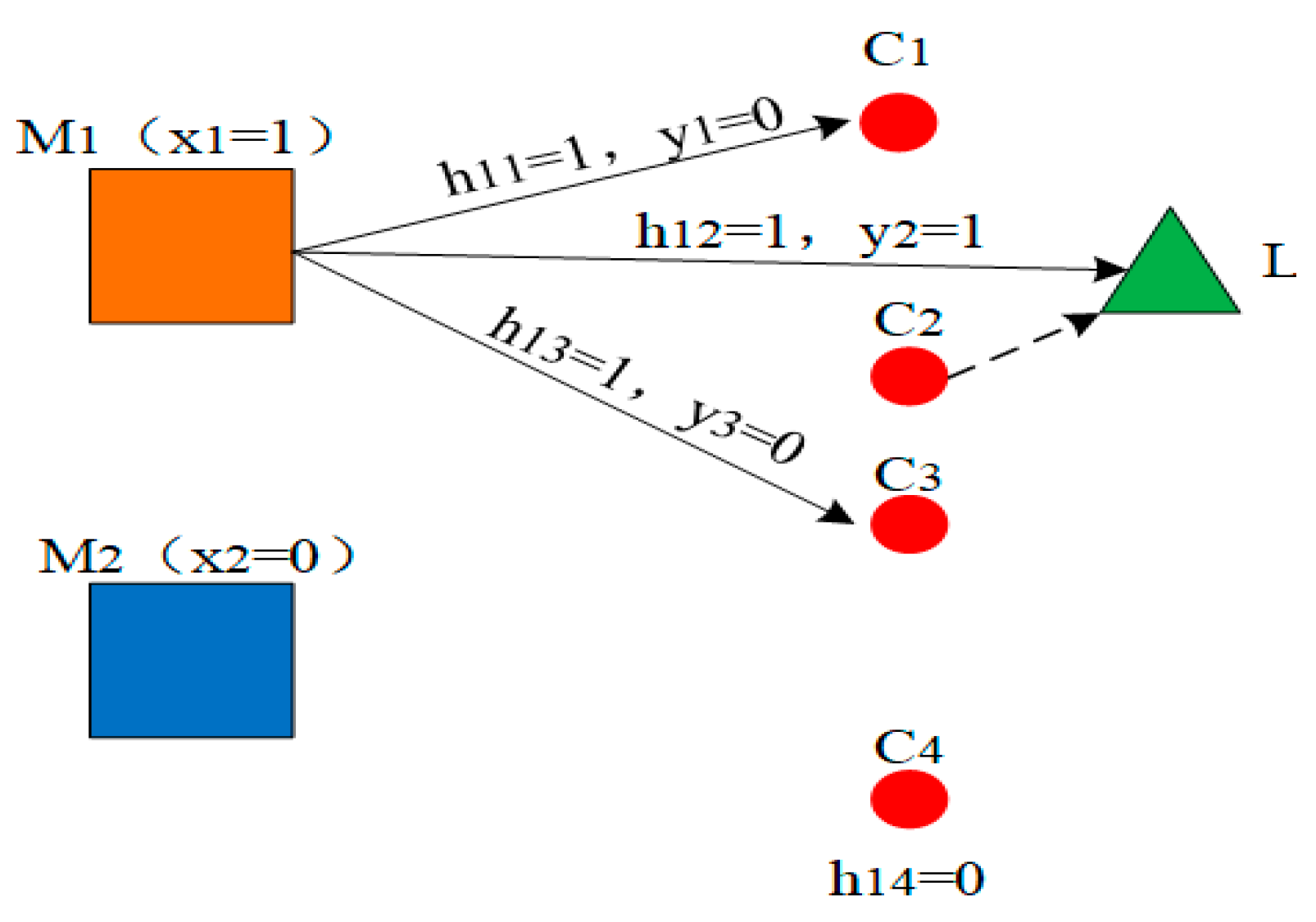
| decision variable | xi | If the alternative point i is the final location of the mini-depot, xi = 1, otherwise, xi = 0. | |
| yj | If the customer point of demand point j is selected to the locker for self-pick-up, yj = 1, Otherwise, customers of customer point j choose the above distribution service, yj = 0. | ||
| hij | If the alternative point i delivers to the customer point demand point j, hij = 1, otherwise, hij = 0. |
| Algorithm Name | Advantages | Disadvantages | Applicable Data Type |
|---|---|---|---|
| AP | (1) No need to pre-specify the number of clusters (2) Automatically identifies representative “exemplars” (3) Applicable to any similarity matrix | (1) High computational complexity (2) Sensitive to the “preference” parameter | Data with any similarity structure |
| K-Means | (1) Simple and efficient (2) Performs well on large datasets (3) Well-established algorithm | (1) Must predefine the number of clusters (2) Only suitable for spherical clusters (3) Sensitive to initial values and outliers | Numerical data, spherical clusters |
| DBSCAN | (1) Can detect noise points | (1) Sensitive to clusters with varying densities | density-separable datasets |
| Number | X(m) | Y(m) | The Tendency Time to Receive the Package | Lj | D2 | Demand | |
|---|---|---|---|---|---|---|---|
| 1 | 448,943.5 | 4,425,062.7 | 0.33 | 16.15637 | 1631 | 537 | 52 |
| 2 | 449,014.5 | 4,425,180.5 | 0.13 | 15.97465 | 1540 | 633 | 93 |
| 3 | 449,104.1 | 4,424,949.5 | 0.52 | 11.73734 | 1750 | 699 | 15 |
| 4 | 449,191.9 | 4,425,079.8 | 0.68 | 17.71023 | 1488 | 522 | 72 |
| 5 | 449,315.3 | 4,425,192.7 | 0.35 | 13.96585 | 1453 | 717 | 61 |
| 6 | 449,378.7 | 4,423,208.5 | 0.57 | 14.92079 | 1556 | 640 | 21 |
| 7 | 448,724.9 | 4,425,187.3 | 0.32 | 11.69148 | 1222 | 603 | 83 |
| 8 | 448,777.2 | 4,425,285.5 | 0.37 | 14.38182 | 1721 | 709 | 87 |
| 9 | 448,662.7 | 4,425,630.1 | 0.69 | 12.07537 | 1299 | 610 | 75 |
| 10 | 448,764.3 | 4,425,791.1 | 0.90 | 13.15929 | 1379 | 603 | 75 |
| 11 | 448,606.3 | 4,425,980.3 | 0.87 | 11.91641 | 1422 | 670 | 88 |
| 12 | 448,771.8 | 4,424,660.7 | 0.29 | 13.40463 | 1641 | 632 | 24 |
| 13 | 448,754.1 | 4,424,844.3 | 0.46 | 15.64142 | 1524 | 792 | 13 |
| 14 | 448,668.0 | 4,424,882.2 | 0.90 | 14.61342 | 1715 | 626 | 22 |
| 15 | 448,726.5 | 4,424,908.1 | 0.33 | 16.57667 | 1215 | 605 | 53 |
| 16 | 448,519.0 | 4,424,917.4 | 0.97 | 15.03617 | 1535 | 591 | 12 |
| 17 | 448,504.7 | 4,424,233.5 | 0.66 | 11.46812 | 1457 | 786 | 88 |
| 18 | 448,542.7 | 4,424,032.1 | 0.25 | 12.73938 | 1696 | 550 | 30 |
| 19 | 448,670.3 | 4,423,407.1 | 0.84 | 17.36076 | 1359 | 528 | 38 |
| 20 | 448,533.0 | 4,423,470.3 | 0.69 | 17.22656 | 1674 | 795 | 22 |
| 21 | 448,362.8 | 4,423,513.6 | 0.59 | 17.92864 | 1579 | 796 | 64 |
| 22 | 448,272.3 | 4,423,621.8 | 0.33 | 13.26559 | 1744 | 713 | 60 |
| 23 | 448,530.6 | 4,423,706.9 | 0.14 | 17.91194 | 1626 | 766 | 21 |
| 24 | 448,696.4 | 4,423,739.2 | 0.31 | 15.29705 | 1467 | 756 | 33 |
| 25 | 448,387.3 | 4,423,583.6 | 0.43 | 15.56457 | 1776 | 600 | 76 |
| 26 | 448,427.7 | 4,423,402.5 | 0.67 | 15.20942 | 1616 | 609 | 58 |
| 27 | 448,232.4 | 4,423,319.5 | 0.99 | 16.58456 | 1367 | 681 | 22 |
| 28 | 448,581.4 | 4,423,227.8 | 0.29 | 15.27313 | 1242 | 500 | 89 |
| 29 | 448,588.0 | 4,423,199.8 | 0.78 | 13.64067 | 1755 | 554 | 49 |
| 30 | 448,608.1 | 4,423,287.0 | 0.90 | 12.22253 | 1484 | 648 | 91 |
| Number | Parameter | Meaning of Parameters | Value |
|---|---|---|---|
| 1 | [CNY/m] | Unit transportation rate of mini-depot delivery to customer demand point. | 0.0003 |
| 2 | F1 [CNY/mini-depot] | Monthly rental cost of a single mini-depot. | 20,000 |
| 3 | F2 [CNY/lockers setting points] | Fixed investment cost of locker facilities. | 400 |
| 4 | r [CNY/m] | The cost of unit power consumption of crowdsourcing battery vehicles. | 0.00008 |
| 5 | e [-] | Distribution compensation coefficient. | 1.5 |
| 6 | [-] | Crowdsourcing distributor distribution range coefficient. | 1.2 |
| 7 | Q [unit] | Maximum capacity of a single locker. | 60 |
| 8 | v [m/s] | The average delivery speed of crowdsourcing distributors. | 5 |
| 9 | α [-] | Cost-satisfaction trade-off coefficient. | 20 |
| 10 | β [-] | Spatio-temporal coefficient that controls the influence degree from space and time dimensions | 0.6 |
| 10 | γ [-] | Positive time sensitivity coefficient of customer satisfaction in door-to-door delivery service. | 0.8 |
| 11 | θ [-] | Distance sensitivity coefficient. | 0.0025 |
| 12 | Lj [s] | The maximum waiting time that customers can accept. | 1800 |
| 13 | D1 [m] | Maximum distance constraint from mini-depot to customer demand point. | 8000 |
| Scenario | Total Cost | Customer Satisfaction | Number of Mini-DEPOT Locations |
|---|---|---|---|
| 1 | 3,375,503.24 | 0.9067 | 16 |
| 2 | 1,481,096.87 | 0.9623 | 43 |
| 3 | 1,565,117.91 | 0.9299 | 40 |
| Scenario | Silhouette | Davies-Bouldin | Calinski-Harabasz | Clusters |
|---|---|---|---|---|
| 1 | −0.180402 | 89.751462 | 1.317687 | 32 |
| 2 | 0.381373 | 0.781603 | 1741.484502 | 68 |
| Scenario | Clusters Mean | Clusters Std | ARI Mean | ARI Std |
|---|---|---|---|---|
| 1 | 32.0 | 0.0 | 1.0 | 0.0 |
| 2 | 68.0 | 0.0 | 1.0 | 0.0 |
| Algorithm | (Population Size, Max Iterations) | Other Parameters | Optimization Method |
|---|---|---|---|
| AHEEFO | (40, 200) | nil | Grid Search |
| EEFO | (40, 200) | nil | Grid Search |
| SSA | (34, 200) | PD = 0.60; SD = 0.28; R2 = 0.74. | Bayesian Optimization |
| WOA | (40, 200) | nil | Grid Search |
| GA | (20, 200) | Crossover rate = 0.76; Mutation rate = 0.08. | Bayesian Optimization |
| PSO | (34, 200) | w = 0.40; c1 = 1.94 c2 = 1.56 | Bayesian Optimization |
| (, ) | Algorithm | AHEEFO | EEFO | SSA | WOA | GA | PSO |
|---|---|---|---|---|---|---|---|
| (0.2,1.5) | Mean value | 1,417,576 | 1,432,491 | 1,459,620 | 1,492,400 | 1,488,484 | 1,433,053 |
| Standard deviation | ±8261.6 | ±14,952.1 | ±13,509.3 | ±40,016.3 | ±14,897.4 | ±17,095.5 | |
| (0.1,2.0) | Mean value | 1,417,620 | 1,433,596 | 1,459,701 | 1,485,659 | 1,488,404 | 1,477,020 |
| Standard deviation | ±14,626.6 | ±21,676.1 | ±15,234.4 | ±34,256.5 | ±17,103.3 | ±19,833.6 | |
| Single operation time (s) | 112.47 | 149.43 | 259 | 224 | 1256 | 137 |
| Algorithm | AHEEFO | EEFO | SSA | WOA | GA | PSO |
|---|---|---|---|---|---|---|
| AHEEFO | - | ★ | ★ | ★ | ★ | ★ |
| EEFO | △ | - | ★ | ★ | ★ | - |
| SSA | △ | △ | - | ★ | ★ | △ |
| WOA | △ | △ | △ | - | - | △ |
| GA | △ | △ | △ | - | - | △ |
| PSO | △ | - | ★ | ★ | ★ | - |
| Scenario | α Value | Constraint Satisfied Mean | Magnitude Gap Mean | Mean | Mean |
|---|---|---|---|---|---|
| 1 | 20 | 1 | 0.538 | 3,896,613.90 | 1,128,920.19 |
| 50 | 1 | 0.1387 | 3,909,038.43 | 2,840,070.37 | |
| 100 | 0 | −0.1616 | 3,960,680.98 | 5,745,574.59 | |
| 200 | 0 | −0.4501 | 4,180,888.99 | 11,785,445.12 | |
| 1000 | 0 | −1.1139 | 4,618,779.22 | 60,034,199.43 | |
| 2 | 20 | 1 | 0.34 | 2,625,128.86 | 1,199,771.09 |
| 50 | 0 | −0.0584 | 2,622,703.97 | 2,999,772.08 | |
| 100 | 0 | −0.359 | 2,626,513.06 | 6,002,424.41 | |
| 200 | 0 | −0.6586 | 2,638,413.48 | 12,019,660.53 | |
| 1000 | 0 | −1.354 | 2,662,292.01 | 60,153,899.15 | |
| 3 | 20 | 1 | 0.3353 | 2,589,424.86 | 1,196,358.33 |
| 50 | 0 | −0.063 | 2,588,782.32 | 2,992,596.87 | |
| 100 | 0 | −0.3633 | 2,594,255.90 | 5,988,325.08 | |
| 200 | 0 | −0.6627 | 2,609,663.13 | 12,002,277.04 | |
| 1000 | 0 | −1.3557 | 2,652,142.83 | 60,151,365.05 |
Disclaimer/Publisher’s Note: The statements, opinions and data contained in all publications are solely those of the individual author(s) and contributor(s) and not of MDPI and/or the editor(s). MDPI and/or the editor(s) disclaim responsibility for any injury to people or property resulting from any ideas, methods, instructions or products referred to in the content. |
© 2025 by the authors. Licensee MDPI, Basel, Switzerland. This article is an open access article distributed under the terms and conditions of the Creative Commons Attribution (CC BY) license (https://creativecommons.org/licenses/by/4.0/).
Share and Cite
Bi, H.; Yang, H.; Lu, F. A Two-Stage Location Problem with Lockers and Mini-Depots Under Crowdsourced Last Mile Delivery in E-Commerce Logistics. J. Theor. Appl. Electron. Commer. Res. 2025, 20, 318. https://doi.org/10.3390/jtaer20040318
Bi H, Yang H, Lu F. A Two-Stage Location Problem with Lockers and Mini-Depots Under Crowdsourced Last Mile Delivery in E-Commerce Logistics. Journal of Theoretical and Applied Electronic Commerce Research. 2025; 20(4):318. https://doi.org/10.3390/jtaer20040318
Chicago/Turabian StyleBi, Hualing, Hengjian Yang, and Fuqiang Lu. 2025. "A Two-Stage Location Problem with Lockers and Mini-Depots Under Crowdsourced Last Mile Delivery in E-Commerce Logistics" Journal of Theoretical and Applied Electronic Commerce Research 20, no. 4: 318. https://doi.org/10.3390/jtaer20040318
APA StyleBi, H., Yang, H., & Lu, F. (2025). A Two-Stage Location Problem with Lockers and Mini-Depots Under Crowdsourced Last Mile Delivery in E-Commerce Logistics. Journal of Theoretical and Applied Electronic Commerce Research, 20(4), 318. https://doi.org/10.3390/jtaer20040318


