Abstract
The aim of the present study is to investigate the multiple slip effects on magnetohydrodynamic unsteady Maxwell nanofluid flow over a permeable stretching sheet with thermal radiation and thermo-diffusion in the presence of chemical reaction. The governing nonlinear partial differential equations are transformed into a system of coupled nonlinear ordinary differential equations with the aid of appropriate similarity variables, and the transformed equations are then solved numerically by using a variational finite element method. The effects of various physical parameters on the velocity, temperature, solutal concentration, and nanoparticle concentration profiles as well as on the skin friction coefficient, rate of heat transfer, and Sherwood number for solutal concentration are discussed by the aid of graphs and tables. An exact solution of flow velocity, skin friction coefficient, and Nusselt number is compared with the numerical solution obtained by FEM and also with numerical results available in the literature. A good agreement between the exact and numerical solution is observed. Also, to justify the convergence of the finite element numerical solution, the calculations are carried out by reducing the mesh size. The present investigation is relevant to high-temperature nanomaterial processing technology.
1. Introduction
The investigation of unsteady Maxwell nanofluid flow over a stretched surface has significantly expanded in recent decades due to several applications in engineering and physical processes. These include microelectromechanical systems (MEMS), advanced nuclear system, combustion chambers, nuclear plants, aircraft, nanoelectromechanical systems (NEMS), fuel cells, glass fiber, and paper production, which play an important role in our daily lives. Daily, several vehicles and devices generate a large quantity of energy, which influences the general activities of the vehicles and devices. Due to energy loss and the requirement to maintain the daily use of the appliance, we need a system which can achieve maximum productivity with minimum wasted expense. The concept of nanofluid (nanoparticles) was first introduced by Choi [1], to describe that base fluid (water, kerosene, biofluids, and ethylene–glycol mixture) enhance thermal conductivity when nanoparticles are added. The thermal conductivity increases when nanoparticles are added, as described by the authors of [2,3,4,5]. Rashidi et al. [6] examined the Brownian and thermophoresis effects on the thermal boundary layer. Akbari et al. [7] examined the influence of nanoparticles on non-Newtonian nanofluids, and they described that the thermal conductivity enhances due to the increase in nanoparticle number. Similar nanoparticle behavior was examined by Mohyud-Din et al. [8] and Hayat et al. [9].
The investigation of nonlinear thermal radiative fluid flow is an area of interest for researchers because of its applications in many engineering processes. Especially, the thermal radiation impact assumes an essential job in controlling the heat transfer process in the polymer processing industry [10]. Raza et al. [11] investigated the entropy generation in the presence of nanoparticles and nonlinear thermal radiation. Mahanthesh et al. [12] investigated the nonlinear thermal radiation effects on magnetohydrodynamic Casson fluid flow. Ismail et al. [13] examined the nonlinear radiation effects on nanofluid slip flow in porous media. The study of nonlinear radiation heat transfer plays an important role in industrial applications at high temperature [14]. Slip condition on stretching surfaces is important in several manufacturing processes. It was found that when the flow pressure is low, the slip boundary condition is necessary. A slip condition on stretching or shrinking surfaces is used by several researchers [15,16,17,18,19]. Ramaya et al. [15] analyzed the nanofluids through a stretching sheet. They observed that the velocity of fluid increases when slip parameter values enhance and slip condition is helpful to control fluid velocity. Khalil et al. [20] conducted a numerical solution of magnetohydrodynamics Casson nanofluid flow. The effect of thermal radiation on the velocity and temperature of a stretching porous thin sheet was studied by Asmat et al. [21]. Chamkha et al. [22] carried out an investigation on heat and mass transfer in a porous medium with a chemical reaction. They obtained a similarity solution for unsteady flow.
The study of magnetohydrodynamics (MHD) with heat transfer flow over a permeable stretching or shrinking sheet is important in many manufacturing processes in the industry, such as in specific applications like polymer processing technology and laser devices used in medical treatment. Daniel et al. [23] studied the free or mixed convection magnetohydrodynamic flow over a sheet. They investigated the numerical solution of free convection and the effects of various physical parameters of interest using the homotopy analysis method. Dhanai et al. [24] conducted multiple solutions of magnetohydrodynamic heat transfer and boundary layer flow over a permeable sheet with viscous dissipation. Gireesha et al. [25] use a dusty fluid to check the flow and heat transfer of magnetohydrodynamic fluid. Haile et al. [26] studied the heat and mass transfer fluid flow in the presence of nanoparticles. They consider unsteady 2D flow and fluid passing along a vertical stretching sheet.
The boundary layer fluids flow caused by the stretching/shrinking surface is an important type of flow occurring in engineering and chemical industries flow processes. These include paper production, liquid metal, glass fiber, and polymer sheet synthesis. The manufacture of non-Newtonian fluids, including lubricants, physiological liquids, paints, colloidal liquids, biological liquids, biopolymers, and foodstuffs, plays an important role in our daily lives. Ashraf et al. [27] investigated the micropolar fluid flow toward a shrinking surface and also studied the radiation effects on thermal conductivity. Dhanai et al. [28] conducted multiple solutions of MHD heat transfer flow with viscous dissipation. The study of unsteady an axisymmetric flow and heat transfer of non-Newtonian fluid over a radially stretching sheet has considered by Shahzad et al. [29]. They also studied the radiation effects on the thermal boundary layer. Ashraf et al. [30] examined the magnetohydrodynamic flow and heat transfer in a micropolar fluid using the stretchable disk. They obtained the numerical solution of an axisymmetric flow over a stretchable disk. Azeem et al. [31] analyzed the heat transfer of an axisymmetric viscous fluid over a nonlinear radially stretching sheet.
The study of free convection or mixed convection flow is important in the electronics cooling process, heat exchangers, etc. Chen [32] examined the laminar mixed convection flow over a continuously stretching sheet. Many researchers engaged in analyzing the mixed convection flow of non-Newtonian fluids [33,34,35,36,37]. Elahi et al. [38] described the numerical solution of mixed convection heat transfer over a stretching sheet. Hayat et al. [39] considered the magnetohydrodynamic flow of non-Newtonian nanofluid flow with the convective condition. They investigated the slip effects on MHD flow of non-Newtonian with a stretching surface. They also found radiation effects on velocity, temperature, and concentration profiles. Baag et al. [40] studied the stagnation point of a magnetohydrodynamic non-Newtonian fluid subject to the chemical reaction and heat source. Singh [41] examined the effects of viscous on free convection non-Newtonian fluid in the presence of chemical reaction. Mabood et al. [42] discussed steady non-Newtonian fluid with a chemical reaction through a porous medium. Hayat et al. [43] discussed a non-Newtonian fluid with chemical aspects and they investigated a numerical solution. Seth et al. [44] examined a chemically reacting nanofluid over a permeable vertical plate.
Motivated by the above literature and the range of applications discussed therein, the study of Unsteady Maxwell Nanofluid Flow and thermo-diffusion with regard to the multiple slips in the presence of chemical reactions has not been discussed before, to best of the authors’ knowledge. The main aim of the present study was to extend the recently published work of Nayak et al. [45]. The governing nonlinear PDEs are transformed into a set of highly nonlinear ODEs with the aid of suitable similarity transformations, and the nonlinear coupled ODEs are solved numerically with the most popular FEM. The influences of the various physical parameters on the fluid velocity, temperature, and solutal and nanoparticle volume fraction functions are examined in detail for specific cases. An exact solution of flow velocity, skin friction coefficient, and Nusselt number is compared with the numerical solution obtained by FEM and also with numerical results available in the literature. Further, the convergence table of the finite element method is discussed with reference to different mesh sizes.
2. Mathematical Formulation
We consider the unsteady two-dimensional MHD flow of an electrically conducting incompressible viscous flow immersed in nanofluid with the presence of thermal radiation and first-order chemical reaction over a permeable stretching surface. The x-axis is chosen along with the sheet and the y-axis is taken normal to it, as shown in Figure 1. It is assumed that the sheet is moving with nonuniform velocity , chosen along the x-axis. Where a is the stretching rate of sheet and is the positive constant with the property . The magnetic field of strength is assumed to be applied in normal direction with . The magnetic Reynolds number Rex is taken to be very small for most of the fluids in industrial applications so that induced magnetic field is ignored. Let , , , and be the ambient temperature, ambient solutal concentration, and ambient nanoparticle concentration, respectively. , , and are the temperature of the sheet, the concentration, and the nanoparticle volume fraction, respectively, at the surface. , and are assumed to be of the following form (see the work by the authors of [46]).
where , , and are the reference temperature, reference solutal concentration, and reference nanoparticle concentration, respectively, such that , and . The above expressions are valid if .
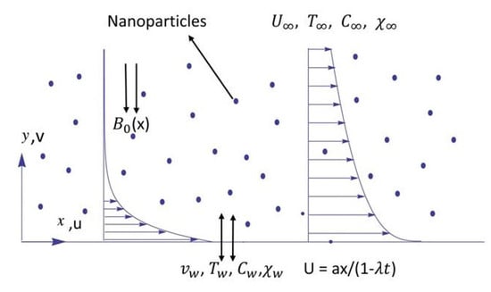
Figure 1.
Physical configuration and coordinate system.
Under the above assumptions, the governing boundary layer equations for the flow problem are as follows (see the works by the authors of [9,19,37,46]).
and the boundary conditions are (see the works by the authors of [46,47])
where u and v are the velocity components along x and y, respectively; , , , and are the thermal diffusivity, kinetic viscosity, electrical conductivity, and density of fluid, respectively; g is the acceleration due to gravity; is thermal expansion coefficient; is the solutal concentration expansion coefficient; is the nanoparticle concentration expansion coefficient; T is the temperature; C is the solutal concentration; is the nanoparticle concentration; is the molecular diffusivity; is the thermal diffusivity; is the Brownian diffusivity; is the Stefan-Boltzmann constant; is the mean absorption coefficient; and are the Soret and Dufour diffusivity, respectively; and is the chemical reaction.
In order to solve Equations (1)–(5), we introduce the following similarity transformations (see the works by the authors of [19,46]).
In view of the similarity transformation in Equation (8), the partial nonlinear differential equations, Equations (1)–(5), transform into the following system of nonlinear ODEs,
and the transformed boundary conditions, Equations (6) and (7), are
The primes shows the differentiation with respect to . The parameters in Equations (9)–(12) are defined as
where is the unsteadiness parameter; M is the magnetic field parameter; is the Prandtl number; is the Brownian motion parameter; is the thermophoresis parameter; is the Deborah number; is the Schmidt number; is the Lewis number; R is the thermal radiation parameter; , , and are the buoyancy parameters; is the permeability parameter; is the chemical reaction parameter; is the Dufour parameter; is the Soret parameter; and is the Suction/injection parameter.
3. Finite Element Method Solutions
Equations (9)–(12) under the boundary conditions (13)–(14) have been solved numerically using the finite element method (FEM). The FEM has been applied to study different problems in computational fluid dynamic and extremely efficient method to solve different nonlinear problems [48,49,50]. Reddy [51] described an excellent general detail of variational finite element method. It has been found that the finite element method is exclusively employed in commercial software like ADINA, ANSYS, MATLAB, and ABAQUS. Swapna et al. and Rana et al. [52,53] described that variational finite element method solves boundary value problem very effectively, quickly, and accurately. We employe the finite element method to the solve nonlinear differential equations, Equations (9)–(12), with the boundary conditions (13)–(14), first we consider
The Equations (9)–(12) thus reduce to
The corresponding boundary conditions reduce to the following form,
3.1. Variational Formulations
The variational form associated with Equations (15)–(19) over a linear element is given by
where and are arbitrary shape function or trial functions.
3.2. Finite Element Formulations
The equation of finite element model is obtained by replacing finite element approximation of the following form in Equations (22)–(26).
with , where the shape function, , for a line element, , is given by
The FE model equations are, therefore, given by
where and (m, n = 1, 2, 3, 4, 5) are defined as
and
where and are supposed to be known. After the assembly of the element Equation (30), the obtained equations are nonlinear, along these lines this requires the utilization of an iterative plan for an effective solution. The functions , , , and are assumed to be known at a lower iteration level to linearize the system and the Gaussian quadrature technique is used to solve the integral. The computations for functions velocity, temperature, solutal and nanofluid volume fraction profile are then completed for higher level, continued until the desired precision of 0.00005 is obtained. The whole algorithm is executed in MATLAB software. To ensure mesh independence, a mesh affectability practice has been performed. No significant variation in the results is noticed for . Therefore, has been fixed at 10. To check the convergence of the results, we calculated the number of elements that increased at , and 2100. The outcomes are delineated in Table 1. It is observed that as n increases beyond 1800, no significant change in the values of velocity, temperature, solutal, and nanoparticles concentration functions is revealed; in this manner, the last outcomes are reported for elements.

Table 1.
Convergence results of the finite element method (FEM) ().
The precise of the existing results, a comparison of the flow velocity is made with the exact solution given by Crane [54] as , under the special case (). The FEM results are a decent concurrence with the exact solution which affirms the validity of FEM. It is clearly seen in Table 2.
Table 2.
Comparison of the exact solution of Crane [54] and FEM for the flow velocity .
4. Results and Discussion
Computations have been performed for quantities of interest like velocity, temperature, and solutal and nanofluid volume fraction for various values of physical parameters. In Table 3, the skin friction coefficient obtained by FEM is compared with the numerical results of Gireesha et al. [25] and the exact solution of Mudassar et al. [55], under special case (). An excellent correlation has been achieved and grid invariance test has been conducted to maintain 4 decimal point accuracy. To ensure the accuracy of the existing numerical results, the skin friction coefficient for steady and unsteady flow obtained by the finite element. We have seen an excellent agreement between our solution and that of the already published research articles; this confirms the validity and accuracy of the present results (see Table 4).
Table 3.
Comparison of skin friction coefficient for various values of M.
Table 4.
Comparison of for various values of M and ().
Table 5 depicts the results of heat transfer rate obtained by FEM compared with the results of pervious studies and exact solution of Ishak et al. [57] under special case (). We noticed that our numerical results are in complete agreement and that the grid invariance test has been conducted to maintain 4 decimal point accuracy. In Table 6, the local skin friction coefficient , the rates of heat transfer and mass transfer − at the surface obtained by FEM is also compared with the already publish research work. A good correlation has been achieved.
Table 5.
Comparison of for various values of ().
Table 6.
Comparison of , , and for various values of Pr and Sc ().
Figure 2 shows the effect of M on the velocity function with no hydrodynamic slip (Figure 2a) and with hydrodynamic slip (Figure 2b). The results show that the velocity component decreases with the increment of M in both cases. Physically, the M produced Lorentz force slowed the motion of the fluid. However, the presence of the hydrodynamic slip, as shown in Figure 2b, decreases the velocity boundary layer. Figure 2 also shows that suction, , causes a reduction in the momentum boundary layer thickness, and thus it provides control over this momentum boundary layer thickness.
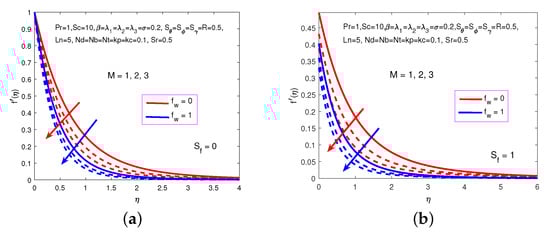
Figure 2.
Influence of M and on . (a) No hydrodynamic slip. (b) With hydrodynamic slip.
Figure 3 and Figure 4 illustrate that the velocity increases with the increment in values of the buoyancy parameters in presence of no hydrodynamic slip (Figure 3 and Figure 4a) and hydrodynamic slip (Figure 3 and Figure 4b). Expanding the estimations of the buoyancy parameters leads to growth of the velocity profile. Physically, the buoyancy supporting forces are strengthened with these increments in buoyancy parameters. We additionally see in Figure 3 that the velocity profile declines reciprocally to as the unsteadiness parameter. It is noticed that the increment in radiation parameter R causes the profile of velocity to enhance. Also increment in hydrodynamic slip causes the profile of the velocity to decrease (Figure 3 and Figure 4b).
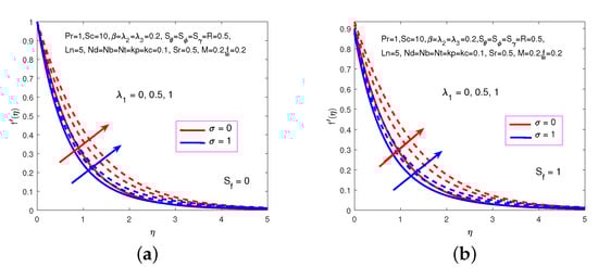
Figure 3.
Influence of and on . (a) No hydrodynamic slip. (b) With hydrodynamic slip.
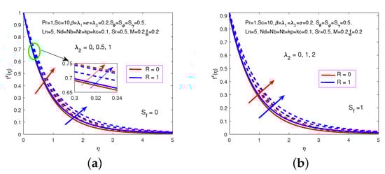
Figure 4.
Influence of and R on . (a) No hydrodynamic slip. (b) With hydrodynamic slip.
A similar behavior of nanoparticle concentration is noticed for buoyancy parameter buoyancy parameter , unsteadiness parameter, and hydrodynamic slip is observed in Figure 5. The influence of varying the permeability parameter on the velocity profile is depicted in Figure 6. We observe in Figure 6 that, as the permeability increases, it causes a decrease in the velocity profile. However, the presence of the hydrodynamic slip, as noticed from Figure 6b decreases the velocity boundary layer. We also observe in Figure 6 that suction reduce the momentum boundary layer thickness. A similar behaviour of Deborah number, , is observed in the velocity profile, as in Figure 7.
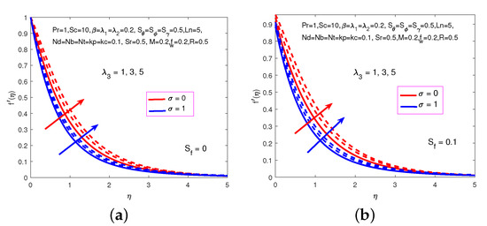
Figure 5.
Influence of and on . (a) No hydrodynamic slip. (b) With hydrodynamic slip.
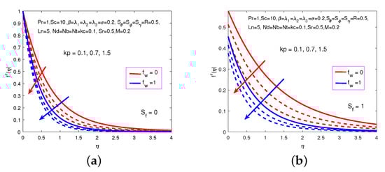
Figure 6.
Influence of and on . (a) No hydrodynamic slip. (b) With hydrodynamic slip.
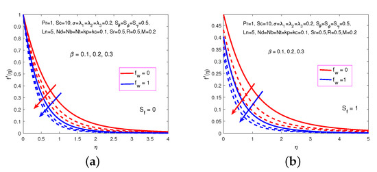
Figure 7.
Influence of and on . (a) No hydrodynamic slip. (b) With hydrodynamic slip.
Figure 8 demonstrates the influence of M on the temperature profile with no thermal slip (Figure 8a) and thermal slip (Figure 8b). The figure shows that the temperature profile increases with the increase of M. Physically, applying the magnetic field warms up the liquid and in this way diminishes the warmth and mass exchange rates from the boundary causing increments in liquid temperature. Figure 8a,b also demonstrates that suction, , and thermal slip decrease the thermal boundary layer thickness. A similar behaviour of Brownian motion is observed on temperature profile as in Figure 9. Brownian motion will be more prominent and Nb will have large values for small size nanoparticles. Consequently, we see that temperatures are upgraded with higher Nb values.
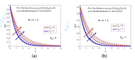
Figure 8.
Influence of M and on . (a) No thermal slip. (b) With thermal slip.
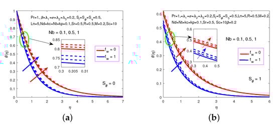
Figure 9.
Influence of and on . (a) No thermal slip. (b) With thermal slip.
Figure 10 shows that decreases of the solutal profile are associated with the increase of . Expanding estimations of the unsteadiness parameters lead to decline in concentration profile. We additionally see in Figure 10b that the concentration profile decline as the solutal slip parameter increments. Figure 11 demonstrates the influence of Soret parameter on the solutal profile. It is clear from Figure 11 that the boundary layer of solutal profile increases with an increment in . A similar behavior of unsteadiness parameter, and solutal slip is observed in Figure 11.
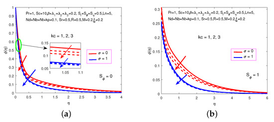
Figure 10.
Influence of and on . (a) No solutal slip. (b) With solutal slip.
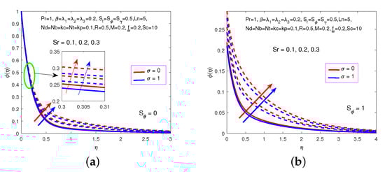
Figure 11.
Influence of and on . (a) No solutal slip. (b) With solutal slip.
Figure 12 shows the influence of on the nanoparticle volume fraction profile with no nanoparticle concentration slip (Figure 12a) and nanoparticle concentration slip (Figure 12b). The nanoparticle volume fraction profile decreases with the increase of . The effects of over the nanoparticle volume fraction profile is also depict in Figure 12b and it is observed that nanoparticle volume fraction profile decreases in unsteady cases. We also see in Figure 12b that the nanoparticles concentration profile decline as the incremented. Figure 13 demonstrates the influence of Lewis number , slip parameter and suction parameter on nanoparticle volume fraction profile is observed, and some interesting observations of nanoparticle volume fraction profile are made. It is clear from Figure 13 that the boundary layer of nanoparticle volume fraction profile decreases with an increment in , , and . Figure 14 shows the influence of M, , , , and on the skin friction coefficient. It is clear from the Figure 14 that skin friction coefficient decreases with increasing values of the slip parameter and buoyancy parameter but skin friction coefficient increases with increasing values of the magnetic, unsteadiness, and suction parameters. The Nusselt number increases with increasing values of magnetic and thermal buoyancy parameters and decreases with increasing values of thermal slip, solutal buoyancy, suction and radiation parameters. It is clearly seen in Figure 15. Figure 16 illustrate the influence of M,, , , and on the reduced Sherwood number. It is clear from Figure 16 that the Sherwood number increases with increasing values of the Schmidt number, unsteadiness, and suction parameters, whereas a reduced Sherwood number decreases with increasing values of the Soret number, magnetic, and solutal slip parameters.
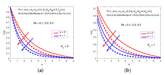
Figure 12.
Influence of and on . (a) No nanoparticles concentration slip. (b) With nanoparticles concentration slip.
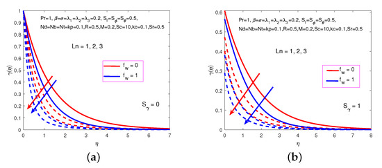
Figure 13.
Influence of and on . (a) No nanoparticles concentration slip. (b) With nanoparticles concentration slip.
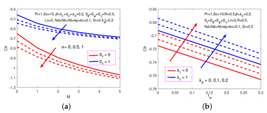
Figure 14.
Influence of , and on the skin friction coefficient. (a) No hydrodynamic slip and with hydrodynamic slip. (b) No thermal buoyancy and with thermal buoyancy.
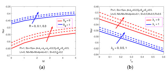
Figure 15.
Influence of , and on the reduced Nusselt number. (a) No thermal slip and with thermal slip. (b) No thermal buoyancy and with thermal buoyancy.
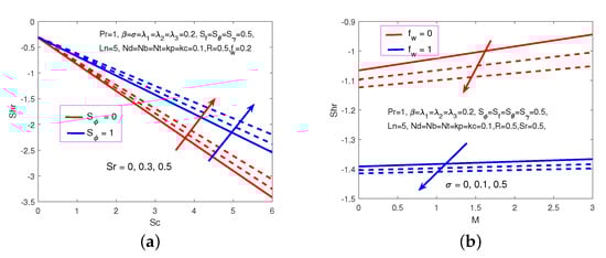
Figure 16.
Influence of , and on the reduced Sherwood number. (a) No solutal slip and with solutal slip. (b) No suction and with suction.
5. Conclusions
The present study analyzes the multiple slip effects on magnetohydrodynamic unsteady Maxwell Nanofluid flow over a permeable stretching sheet with radiation and thermo-diffusion in the presence of chemical reaction. By using the appropriate similarity transformation, the control nonlinear PDEs are transformed into a set of highly nonlinear ODEs, and the nonlinear coupled ODEs are solved by using robust and verified variational finite element method under the realistic boundary conditions. The computations have been performed for velocity, temperature, solutal and nanofluid volume fraction functions for various values of physical parameters. The key conclusions of this work are as follows.
- The velocity profiles decrease with increasing values of suction, slip, unsteadiness, magnetic, Deborah number, and permeability parameters, but the influence is opposite for increasing values of buoyancy parameters and thermal radiation.
- Increments in magnetic field and Brownian motion parameters enhance the fluid temperature. However, the opposite influence is experienced with increasing values of suction and slip parameters.
- The solutal profle reduces with increasing values of the chemical reaction parameter, unsteadiness parameter, and slip parameter, but the solutal profile is enhanced with increasing values Soret number.
- Increasing the values of the thermophoresis, suction, slip, Lewis number, and unsteady parameters leads to the deceleration of the nanoparticles volume fraction profile.
- The skin friction coefficient increases with increasing rates of magnetic, suction, and unsteadiness parameters, whereas the skin friction coefficient decreases with the higher values of the slip and buoyancy parameters.
- Increments in magnetic field and thermal buoyancy parameters enhance the fluid Nusselt number but the opposite influence is experienced with increasing values of slip, solutal buoyancy, suction, and thermal radiation parameters.
- The Sherwood number increases with increasing values of Schmidt number, unsteadiness, and suction parameters, but reduces with increasing values of the Soret number, magnetic, and slip parameters.
Author Contributions
B.A. and S.A.K. modeled the problem and wrote the manuscript. Y.N. thoroughly checked the mathematical modeling and English corrections. B.A. solved the problem using MATLAB software. M.T.S. and M.T.: writing—review and editing. Y.N. contributed to the results and discussions. All authors finalized the manuscript after its internal evaluation.
Funding
This research was funded by the National Natural Science Foundation of China (Grant No. 11971386).
Conflicts of Interest
The authors declare no conflicts of interest.
References
- Choi, S. Enhancing thermal conductivity of fluids with nanoparticle. In Development and Applications of Non-Newtonian Flow; 1995; Volume 31, pp. 99–105. Available online: https://pdfs.semanticscholar.org/06b5/8dc033ac26296c9231cc7b2b48611efb2ca8.pdf (accessed on 15 September 2019).
- Rao, A.S.; Prasad, V.R.; Nagendra, N.; Murthy, K.V.N.; Reddy, N.B. Numerical Modeling of Non-Similar Mixed Convection Heat Transfer over a Stretching Surface with Slip Conditions. World J. Mech. 2015, 5, 117–128. [Google Scholar] [CrossRef]
- Rana, P.; Bhargava, R. Numerical study of heat transfer enhancement in mixed convection flow along a vertical plate with heat source/sink utilizing nanofluids. Commun. Nonlinear Sci. Numer. Simul. 2011, 16, 4318–4334. [Google Scholar] [CrossRef]
- Hayat, T.; Khan, M.I.I.; Qayyum, S.; Alsaedi, A.; Khan, M.I.I. New thermodynamics of entropy generation minimization with nonlinear thermal radiation and nanomaterials. Phys. Lett. Sect. A Gen. At. Solid State Phys. 2018, 382, 749–760. [Google Scholar] [CrossRef]
- Mabood, F.; Ibrahim, S.M.; Khan, W.A. Effect of melting and heat generation/absorption on Sisko nano fluid over a stretching surface with nonlinear radiation. Phys. Scr. 2019, 94, 065701. [Google Scholar] [CrossRef]
- Rashidi, M.M.; Bagheri, S.; Momoniat, E.; Freidoonimehr, N. Entropy analysis of convective MHD flow of third grade non-Newtonian fluid over a stretching sheet. Ain Shams Eng. J. 2017, 8, 77–85. [Google Scholar] [CrossRef]
- Akbari, O.A.; Toghraie, D.; Karimipour, A.; Marzban, A.; Ahmadi, G.R. The effect of velocity and dimension of solid nanoparticles on heat transfer in non-Newtonian nanofluid. Phys. E Low-Dimens. Syst. Nanostructures 2017, 86, 68–75. [Google Scholar] [CrossRef]
- Mohyud-Din, S.T.; Khan, U.; Ahmed, N.; Rashidi, M.M. A study of heat and mass transfer on magnetohydrodynamic (MHD) flow of nanoparticles. Propuls. Power Res. 2018, 7, 72–77. [Google Scholar] [CrossRef]
- Hayat, T.; Ahmad, S.; Khan, M.I.; Alsaedi, A. Results in Physics Simulation of ferromagnetic nanomaterial flow of Maxwell fluid. Results Phys. 2018, 8, 34–40. [Google Scholar] [CrossRef]
- Pal, D. Combined effects of non-uniform heat source/sink and thermal radiation on heat transfer over an unsteady stretching permeable surface. Commun. Nonlinear Sci. Numer. Simul. 2011, 16, 1890–1904. [Google Scholar] [CrossRef]
- Raza, J. Thermal radiation and slip effects on magnetohydrodynamic (MHD) stagnation point flow of Casson fluid over a convective stretching sheet. Propuls. Power Res. 2019, 8, 138–146. [Google Scholar] [CrossRef]
- Mahanthesh, B.; Gireesha, B.J.; Thammanna, G.T.; Shehzad, S.A.; Abbasi, F.M.; Gorla, R.S.R. Nonlinear convection in nano Maxwell fluid with nonlinear thermal radiation: A three-dimensional study. Alex. Eng. J. 2018, 57, 1927–1935. [Google Scholar] [CrossRef]
- Ismail, A.I. Finite element simulation of magnetohydrodynamic convective nanofluid slip flow in porous media with nonlinear radiation. Alex. Eng. J. 2016, 55, 1305–1319. [Google Scholar] [CrossRef]
- Rana, P.; Dhanai, R.; Kumar, L. Radiative nanofluid flow and heat transfer over a nonlinear permeable sheet with slip conditions and variable magnetic field: Dual solutions. Ain Shams Eng. J. 2017, 8, 341–352. [Google Scholar] [CrossRef][Green Version]
- Ramya, D.; Raju, R.S.; Rao, J.A.; Rashidi, M.M. Boundary layer Viscous Flow of Nanofluids and Heat Transfer Over a Nonlinearly Isothermal Stretching Sheet in the Presence of Heat Generation/Absorption and Slip Boundary Conditions. Int. J. Nanosci. Nanotechnol. 2016, 12, 251–268. [Google Scholar]
- Amanulla, C.H.; Nagendra, N.; Reddy, M.S. Computational analysis of non-Newtonian boundary layer flow of nanofluid past a semi-infinite vertical plate with partial slip. Nonlinear Eng. 2018, 7, 29–43. [Google Scholar] [CrossRef]
- Bég, O.A.; Basir, M.F.M.; Uddin, M.J.; Ismail, A.I.M. Numerical Study of Slip Effects on Unsteady Asymmetric Bioconvective Nanofluid Flow in a Porous Microchannel With an Expanding/Contracting Upper Wall Using Buongiorno’s Model. J. Mech. Med. Biol. 2016, 17, 1750059. [Google Scholar] [CrossRef]
- Hayat, T.; Nassem, A.; Khan, M.I.; Farooq, M.; Al-Saedi, A. Magnetohydrodynamic (MHD) flow of nanofluid with double stratification and slip conditions. Phys. Chem. Liq. 2018, 56, 189–208. [Google Scholar] [CrossRef]
- Malarselvi, A.; Bhuvaneswari, M.; Sivasankaran, S.; Ganga, B.; Hakeem, A.K.A. Effect of Slip and Convective Heating on Unsteady MHD Chemically Reacting Flow Over a Porous Surface with Suction. In Applied Mathematics and Scientific Computing; Birkhauser: Cham, Switzerland, 2019; pp. 357–365. [Google Scholar]
- Rehman, K.U.; Malik, M.Y.; Zahri, M.; Tahir, M. Numerical analysis of MHD Casson Navier’s slip nanofluid flow yield by rigid rotating disk. Results Phys. 2018, 8, 744–751. [Google Scholar] [CrossRef]
- Ara, A.; Khan, N.A.; Khan, H.; Sultan, F. Radiation effect on boundary layer flow of an Eyring-Powell fluid over an exponentially shrinking sheet. Ain Shams Eng. J. 2014, 5, 1337–1342. [Google Scholar] [CrossRef]
- Chamkha, A.J.; Aly, A.M.; Mansour, M.A.; Education, A.; Valley, S. Similarity solution for unsteady heat and mass transfer from a stretching surface embedded in a porous medium with suction/injection and chemical reaction. Chem. Eng. Commun. 2010, 197, 37–41. [Google Scholar] [CrossRef]
- Daniel, Y.S.; Daniel, S.K. Effects of buoyancy and thermal radiation on MHD flow over a stretching porous sheet using homotopy analysis method. Alex. Eng. J. 2015, 54, 705–712. [Google Scholar] [CrossRef]
- Dhanai, R.; Rana, P.; Kumar, L. Multiple solutions of MHD boundary layer flow and heat transfer behavior of nanofluids induced by a power-law stretching/shrinking permeable sheet with viscous dissipation. Powder Technol. 2015, 273, 62–70. [Google Scholar] [CrossRef]
- Gireesha, B.J.; Ramesh, G.K.; Bagewadi, C.S. Heat transfer in MHD flow of a dusty fluid over a stretching sheet with viscous dissipation. J. Appl. Sci. Res. 2012, 3, 2392–2401. [Google Scholar]
- Haile, E.; Shankar, B. Heat and Mass Transfer in the Boundary Layer of Unsteady Viscous Nanofluid along a Vertical Stretching Sheet. J. Comput. Eng. 2014, 2014, 1–17. [Google Scholar] [CrossRef]
- Ashraf, M.; Bashir, S. Numerical simulation of MHD stagnation point flow and heat transfer of a micropolar fluid towards a heated shrinking sheet. Int. J. Numer. Methods Fluids 2012, 69, 384–398. [Google Scholar] [CrossRef]
- Dhanai, R.; Rana, P.; Kumar, L. Critical values in slip flow and heat transfer analysis of non-Newtonian nanofluid utilizing heat source/sink and variable magnetic field: Multiple solutions. J. Taiwan Inst. Chem. Eng. 2016, 58, 155–164. [Google Scholar] [CrossRef]
- Shahzad, A.; Ali, R.; Hussain, M.; Kamran, M. Unsteady axisymmetric flow and heat transfer over time-dependent radially stretching sheet. Alex. Eng. J. 2017, 56, 35–41. [Google Scholar] [CrossRef]
- Ashraf, M.; Batool, K. Mhd Flow and Heat Transfer of a Micropolar Fluid Over a Stretchable Disk. J. Theor. Appl. Mech. 2013, 51, 25–38. [Google Scholar]
- Shahzad, A.; Ahmed, J.; Khan, M. On heat transfer analysis of axisymmetric flow of viscous fluid over a nonlinear radially stretching sheet. Alex. Eng. J. 2016, 55, 2423–2429. [Google Scholar] [CrossRef]
- Chen, C.H. Laminar mixed convection adjacent to vertical, continuously stretching sheets. Heat Mass Transf.- Und Stoffuebertragung 1998, 33, 471–476. [Google Scholar] [CrossRef]
- Rana, P.; Bég, O.A. Mixed convection flow along an inclined permeable plate: Effect of magnetic field, nanolayer conductivity and nanoparticle diameter. Appl. Nanosci. 2015, 5, 569–581. [Google Scholar] [CrossRef]
- Thumma, T.; Anwar Bég, O.; Kadir, A. Numerical study of heat source/sink effects on dissipative magnetic nanofluid flow from a nonlinear inclined stretching/shrinking sheet. J. Mol. Liq. 2017, 232, 159–173. [Google Scholar] [CrossRef]
- Seth, G.S.; Sarkar, S. MHD natural convection heat and mass transfer flow past a time dependent moving vertical plate with ramped temperature in a rotating medium with hall effects, radiation and chemical reaction. J. Mech. 2015, 31, 91–104. [Google Scholar] [CrossRef]
- Takhar, H.S.; Agarwal, R.S.; Bhargava, R.; Jain, S. Mixed convection flow of a micropolar fluid over a stretching sheet. Heat Mass Transf.- Und Stoffuebertragung 1998, 34, 213–219. [Google Scholar] [CrossRef]
- Okedoye, A.M.; Akinrinmade, V.A. MHD Mixed Convection Heat and Mass Transfer Flow from Vertical Surfaces in Porous Media with Soret and Dufour Effects. J. Sci. Eng. Res. 2017, 4, 75–85. [Google Scholar]
- Ellahi, R.; Zeeshan, A.; Shehzad, N.; Alamri, S.Z. Structural impact of kerosene-Al2O3nanoliquid on MHD Poiseuille flow with variable thermal conductivity: Application of cooling process. J. Mol. Liq. 2018, 264, 607–615. [Google Scholar] [CrossRef]
- Hayat, T.; Waqas, M.; Khan, M.I.; Alsaedi, A.; Shehzad, S.A. Magnetohydrodynamic flow of burgers fluid with heat source and power law heat flux. Chin. J. Phys. 2017, 55, 318–330. [Google Scholar] [CrossRef]
- Baag, S.; Mishra, S.R.; Dash, G.C.; Acharya, M.R. Numerical investigation on MHD micropolar fluid flow toward a stagnation point on a vertical surface with heat source and chemical reaction. J. King Saud Univ.-Eng. Sci. 2017, 29, 75–83. [Google Scholar] [CrossRef]
- Singh, K. Effect of Viscous Dissipation on Double Stratified MHD Free Convection in Micropolar Fluid Flow in Porous Media with Chemical Reaction , Heat Generation and Ohmic Heating. Chem. Process. Eng. Res. 2015, 31, 75–81. [Google Scholar]
- Mabood, F.; Shateyi, S.; Rashidi, M.M.; Momoniat, E.; Freidoonimehr, N. MHD stagnation point flow heat and mass transfer of nanofluids in porous medium with radiation, viscous dissipation and chemical reaction. Adv. Powder Technol. 2016, 27, 742–749. [Google Scholar] [CrossRef]
- Hayat, T.; Khan, M.I.; Waqas, M.; Alsaedi, A. Mathematical modeling of non-Newtonian fluid with chemical aspects: A new formulation and results by numerical technique. Colloids Surf. A Physicochem. Eng. Asp. 2017, 518, 263–272. [Google Scholar] [CrossRef]
- Mahanthesh, B.; Gireesha, B.J.; Athira, P.R. Radiated flow of chemically reacting nanoliquid with an induced magnetic field across a permeable vertical plate. Results Phys. 2017, 7, 2375–2383. [Google Scholar] [CrossRef]
- Nayak, B.; Mishra, S.R.; Krishna, G.G. Chemical reaction effect of an axisymmetric flow over radially stretched sheet. Propul. Power Res. 2019, 8, 1–6. [Google Scholar] [CrossRef]
- Mabood, F. Multiple Slip Effects on MHD Unsteady Flow Heat and Mass. Model. Simul. Eng. 2019, 2019, 3052790. [Google Scholar]
- Uddin, M.; Alginahi, Y.; Bég, O.A.; Kabir, M. Numerical solutions for gyrotactic bioconvection in nanofluid-saturated porous media with Stefan blowing and multiple slip effects. Comput. Math. Appl. 2016, 72, 2562–2581. [Google Scholar] [CrossRef]
- Singh, B.; Gupta, D.; Kumar, L.; Anwar, O.B. Finite Element Analysis of MHD Flow of Micropolar Fluid over a Shrinking Sheet with a Convective Surface Boundary Condition. J. Eng. Thermophys. 2018, 27, 202–203. [Google Scholar] [CrossRef]
- Bhargava, R.; Rana, P. Finite element solution to mixed convection in MHD flow of micropolar fluid along a moving vertical cylinder with variable conductivity. Int. J. Appl. Math Mech. 2011, 7, 29–51. [Google Scholar]
- Rana, P.; Bhargava, R.; Bég, O.A. Finite element simulation of unsteady magneto-hydrodynamic transport phenomena on a stretching sheet in a rotating nanofluid. Proc. Inst. Mech. Eng. Part N J. Nanoeng. Nanosyst. 2013, 227, 77–99. [Google Scholar] [CrossRef]
- Reddy, J. Solutions manual for An introduction to the finite element method. In Essentials of Finite Element Method; Elsevier: Amsterdam, The Netherlands, 1993; p. 41. [Google Scholar]
- Swapna, G.; Kumar, L.; Rana, P.; Singh, B. Finite element modeling of a double-diffusive mixed convection flow of a chemically-reacting magneto-micropolar fluid with convective boundary condition. J. Taiwan Inst. Chem. Eng. 2015, 47, 18–27. [Google Scholar] [CrossRef]
- Kumar, L. Finite-element analysis of transient heat and mass transfer in microstructural boundary layer flow from a porous stretching sheet finite-element analysis of transient heat and mass transfer in microstructural boundary layer flow from a porous. Comput. Therm. Sci. Int. J. 2014, 6, 155–169. [Google Scholar] [CrossRef]
- Crane, L.J. Flow past a stretching plate. Z. Für Angew. Math. Und Phys. ZAMP 1970, 21, 645–647. [Google Scholar] [CrossRef]
- Jalil, M.; Asghar, S.; Yasmeen, S. An Exact Solution of MHD Boundary Layer Flow of Dusty Fluid over a Stretching Surface. Math. Probl. Eng. 2017, 2017, 1–5. [Google Scholar] [CrossRef]
- Aii, M.E.; Chamkha, A.J.; Aly, A.M.; Mansour, M.A.; Education, A.; Valley, S.; Mabood, F.; Das, K. Melting heat transfer on hydromagnetic flow of a nanofluid over a stretching sheet with radiation and second-order slip. Eur. Phys. J. Plus 2016, 234, 227–234. [Google Scholar] [CrossRef]
- Ishak, A.; Nazar, R.; Pop, I. Boundary layer flow and heat transfer over an unsteady stretching vertical surface. Meccanica 2009, 44, 369–375. [Google Scholar] [CrossRef]
- Aii, M.E. Heat transfer characteristics of a continuous stretching surface. Warme-und Stoffubertragung 1994, 29, 227–234. [Google Scholar]
© 2019 by the authors. Licensee MDPI, Basel, Switzerland. This article is an open access article distributed under the terms and conditions of the Creative Commons Attribution (CC BY) license (http://creativecommons.org/licenses/by/4.0/).