Optimal Control and Neural Porkchop Analysis for Low-Thrust Asteroid Rendezvous Mission ^†

Abstract

This paper presents a comparative study of the applicability and accuracy of optimal control methods and neural-network-based estimators in the context of porkchop plots for preliminary asteroid rendezvous mission design. The scenario considered involves a deep-space CubeSat equipped with a low-thrust engine, departing from Earth and rendezvousing with a near-Earth asteroid within a three-year launch window. A low-thrust trajectory optimization model is formulated, incorporating variable specific impulse, maximum thrust, and path constraints. The optimal control problem is efficiently solved using Sequential Convex Programming (SCP) combined with a solution continuation strategy. The neural network framework consists of two models: one predicts the minimum fuel consumption ($\Delta v$), while the other estimates the minimum flight time ($\Delta t$) which is used to assess transfer feasibility. Case results demonstrate that, in simplified scenarios without path constraints, the neural network approach achieves low relative errors across most of the design space and successfully captures the main structural features of the porkchop plots. In cases where the SCP-based continuation method fails due to the presence of multiple local optima, the neural network still provides smooth and globally consistent predictions, significantly improving the efficiency of early-stage asteroid candidate screening. However, the deformation of the feasible region caused by path constraints leads to noticeable discrepancies in certain boundary regions, thereby limiting the applicability of the network in detailed mission design phases. Overall, the integration of neural networks with porkchop plot analysis offers an effective decision-making tool for mission designers and planetary scientists, with significant potential for engineering applications.

1. Introduction

Near-Earth asteroids (NEAs) offer unique scientific value for understanding the early evolution of the solar system, assessing extraterrestrial resources [1], and enhancing planetary defense. They also possess engineering value due to their relative accessibility. It is estimated that the number of observable NEAs has exceeded ten thousand, and the number of detectable targets continues to increase rapidly [2]. In recent years, Japan’s Hayabusa-2 mission successfully collected and returned samples from Ryugu, while NASA’s OSIRIS-REx mission obtained samples from Bennu. The DART mission further demonstrated, for the first time, the feasibility of kinetic impactor technology for asteroid deflection [3,4,5]. With the maturation of deep-space CubeSats and small satellite platforms, opportunities for low-cost and low-thrust missions to NEAs are increasing [6,7]. However, such missions must perform complex trajectory design under strict mass and power constraints [8], highlighting the need for more efficient preliminary mission assessment tools.

The “porkchop” plot provides an intuitive cost landscape of fuel consumption and transfer time for interplanetary missions by sweeping departure epochs and flight durations. However, for low-thrust spacecraft, each grid point requires solving an optimal control problem that may involve multiple constraints, variable specific impulse, and other nonlinearities, leading to a computational burden significantly higher than that of chemical propulsion [9,10]. Existing optimal control methods include direct methods such as pseudospectral methods, Sequential Convex Programming (SCP), and dynamic programming [11,12,13,14,15], as well as indirect methods based on Pontryagin’s maximum principle [16,17]. Even with advanced optimal control methods and continuation techniques [18], generating a porkchop plot for a single transfer target through dense sampling can require tens to hundreds of CPU hours, and is sensitive to initial guesses and local minima. This remains computationally prohibitive when applied to a large number of NEA targets.

In recent years, deep learning has been increasingly applied in astrodynamics, using multilayer perceptrons to directly regress fuel consumption or assess reachability [19,20,21,22,23,24,25]. Machine learning models have also been employed for real-time trajectory guidance [26,27,28,29]. Neural networks, with their universal approximation capabilities [30] and microsecond-level inference efficiency, are well-suited to large-sample scenarios such as porkchop plot generation. However, existing studies have mostly focused on specific transfer scenarios, and are often validated under simplified assumptions such as constant thrust and the absence of path constraints. Moreover, quantitative comparisons with advanced optimal control methods are often lacking, especially when addressing realistic engineering constraints such as variable specific impulse, thermal limits, and power restrictions [31,32].

To this end, this study aims to evaluate the accuracy of neural networks (NNs) in realistic, constrained low-thrust mission scenarios, and to assess whether they can serve as a fast surrogate tool for asteroid pre-selection during early mission design, while also clarifying their limitations. A representative scenario—porkchop plot generation for rendezvous missions to near-Earth asteroids—is selected for analysis. The applicability and accuracy of optimal control methods and neural networks are compared in this context.

The main contributions of this paper are summarized as follows:

1.

Under realistic scenarios involving variable specific impulse, maximum thrust, and path constraints, this paper conducts a quantitative accuracy comparison between neural networks and optimal control methods at the porkchop plot level.

2.

Under simple transfer conditions, the neural network maintains a relative error of less than 10% across most of the feasible domain.

3.

The study demonstrates that the porkchop plot is a suitable scenario for applying neural networks. It not only provides fast and direct support for engineering design, but also allows for visual validation of neural network performance across a wide range of transfer scenarios.

The remainder of this paper is organized as follows: Section 2 describes the mission model and algorithms; Section 3 presents the experimental results; Section 4 discusses the sources of error and potential improvements; and Section 5 concludes the paper.

2. Problem Description and Methods

This paper investigates the porkchop plot in the context of a practical asteroid rendezvous mission. The scenario involves a CubeSat launched from Earth to rendezvous with an asteroid. The rocket provides a maximum hyperbolic excess velocity $v_{\infty }^{max}$ of 4 km/s, with no constraint on direction. The departure date ranges from 1 January 2029 to 31 December 2031, with a flight time between 200 and 1200 days and a time step of 10 days. Each point in the porkchop plot represents a computation aimed at minimizing the total velocity increment required for the rendezvous. The initial mass of the satellite is $26.5$ kg, with 2 kg of propellant allocated to the thruster. The maximum thrust and specific impulse of the low-thrust engine vary with the spacecraft’s distance from the Sun. Path constraints are also imposed in this scenario.

This section introduces the optimal control problem corresponding to the porkchop plot analysis of the asteroid rendezvous mission studied in this paper. It covers the definition of the low-thrust trajectory optimization problem, the optimal control method used for its solution, and the neural network model employed for prediction. First, the mathematical formulation of the low-thrust trajectory optimization problem is presented, including the dynamical equations, the modeling of variable specific impulse and maximum thrust, and the path constraints. Then, the optimal control method used to solve the problem, namely the Sequential Convex Programming (SCP) algorithm, is introduced. Finally, the structure and training process of the neural network model are described, along with the indirect method used for data generation, and the approach to use the trained model for prediction.

2.1. Problem Definition

The problem of interest is the optimization of low-thrust trajectories for asteroid rendezvous missions. The objective is to minimize the total velocity increment required for a CubeSat to rendezvous with an asteroid. The equations of motion governing the spacecraft include gravitational forces and thrust forces Γ

$$\begin{array}{cc}\hfill \dot{\mathit{r}}& =\mathit{v}\hfill \end{array}$$

(1)

$$\begin{array}{cc}\hfill \dot{\mathit{v}}& =-{\displaystyle \frac{\mu }{r^3}}\mathit{r}+{\displaystyle \frac{\mathsf{\Gamma }}{m}}\hfill \end{array}$$

(2)

where $\mathit{r}$ is the position vector, $\mathit{v}$ is the velocity vector, $\mu$ is the gravitational parameter of the Sun, $r={\left|\right|\mathit{r}\left|\right|}_2$. Fuel consumption obeys

$$\dot{m}\left(t\right)=-{\displaystyle \frac{\parallel \mathsf{\Gamma }\left(t\right)\parallel }{I_{\mathrm{sp}}\left(t\right)g_0}}$$

(3)

where Γ(t) is the thrust force, $I_{sp}\left(t\right)$ is the specific impulse and $g_0$ is the gravitational acceleration at sea level.

A realistic thruster model is implemented by mapping the maximum thrust $T_{max}$ and specific impulse $I_{sp}$ variation over the instantaneous input power. The available input power P is powered by solar arrays and depends on the spacecraft distance r from the Sun. Polynomial surrogate models of the thruster and power production, derived from experimental measurements, are used to capture the complexities of these systems while maintaining smooth derivatives. The coefficients of the third-order polynomials describing $P\left(r\right)$, $T_{\max }\left(P\right)$ and $I_{sp}\left(P\right)$ are detailed in Table 1. The values correspond to a deep-space CubeSat mission comparable to ESA M-ARGO mission [7].

Table 1. Electric propulsion thruster coefficients.

Input Power Limits	${\mathit{T}}_{\mathbf{max}}$ [$\mathit{\mu }$N/Wi] Coeff.	${\mathit{I}}_{\mathit{sp}}$ [s/Wi] Coeff.	P [W/AUi] Coeff.
$$\begin{gathered} P_{\mathrm{in},\min }=80\mathrm{W} \\ {P}_{\mathrm{in},\max }=130\mathrm{W} \end{gathered}$$	$a_0=-1234.3$	$b_0=-5519.5$	$c_0=1281.4$
	$a_1=26.498$	$b_1=225.44$	$c_1=-2518.8$
	$a_2=0$	$b_2=-1.8554$	$c_2=1828.5$
	$a_3=0$	$b_3=5.0836\times {10}^{-3}$	$c_3=-475.80$

Maximum thrust and specific impulse can also be expressed directly as a function of the distance from the Sun, as shown in Figure 1.

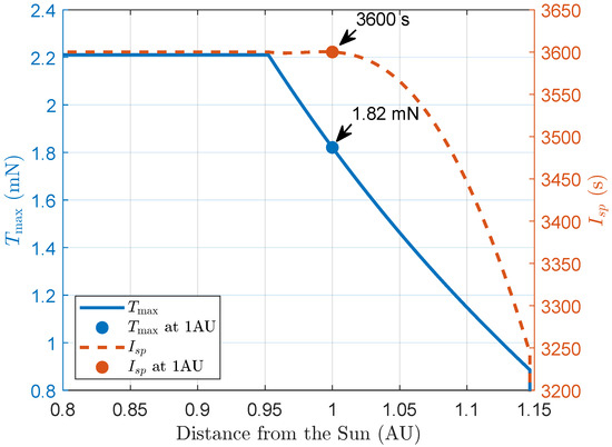
Figure 1. Variable $T_{\max }$ and $I_{\mathrm{sp}}$ curves with respect to the distance from the Sun.

Variations of $T_{max}$ and $I_{\mathrm{sp}}$ with heliocentric distance (in astronomical units, AU) are modeled by fourth order polynomials between 0.9525 AU to 1.1467 AU

$$T_{max}\left(x\right)=\left\{\begin{array}{cc}2.2\times {10}^{-3}\mathrm{N},\hfill & x\le 0.9525,\hfill \\ {\displaystyle \sum _{i=0}^4{c}_{T,i}{x}^i,}\hfill & 0.9525<x<1.1467,\hfill \\ 0,\hfill & x\ge 1.1467,\hfill \end{array}\right.I_{\mathrm{sp}}\left(x\right)=\left\{\begin{array}{cc}3600\mathrm{s},\hfill & x\le 0.9525,\hfill \\ {\displaystyle \sum _{i=0}^4{c}_{I,i}{x}^i,}\hfill & 0.9525<x<1.1467,\hfill \\ 0,\hfill & x\ge 1.1467,\hfill \end{array}\right.$$

(4)

where the thrust coefficients and the $I_{\mathrm{sp}}$ coefficients are summarized in Table 2.

Table 2. Fourth order polynomial coefficients for thrust $T_{max}\left(x\right)$ and specific impulse $I_{\mathrm{sp}}\left(x\right)$.

i	${\mathit{c}}_{\mathit{T},\mathit{i}}$ [N / AUi]	${\mathit{c}}_{\mathit{I},\mathit{i}}$ [s / AUi]
0	$0.0327202372$	$3.1951149396\times {10}^5$
1	$-0.0667431624$	$-1.1891014516\times {10}^6$
2	$0.0484515930$	$1.6645687780\times {10}^6$
3	$-0.0126077484$	$-1.0253620793\times {10}^6$
4	0	$2.3398323687\times {10}^5$

Due to thermal and power constraints, the CubeSat trajectory is required to stay above 0.8 AU, and the engine must be shut down beyond 1.15 AU throughout the mission, representing a path constraint.

2.2. Optimal Control Method

To efficiently analyze the reachability of multiple asteroids, a fast and reliable method is needed to compute thousands of fuel-optimal low-thrust trajectories per target. This work employs a direct Sequential Convex Programming (SCP) algorithm, solving a convex subproblem for each combination of departure date and time of flight. The solution is then used as an initial guess for neighboring problems across the time grid, ensuring robust convergence and smooth porkchop plots. The nonconvex low-thrust trajectory optimization problem is solved by considering a sequence of convex subproblems whose solution converges, under defined hypotheses, to the solution of the original one [13].

At each SCP iteration, the quantities $\tilde{\mathit{x}}\left(t\right)$ and $\tilde{\mathit{u}}\left(t\right)$ denote the reference state and control vectors obtained from the solution of the previous iteration. These reference trajectories are used to build a local convex approximation of the original nonconvex problem through first-order linearization. Exploiting a correct change of variables and convexification techniques, at each iteration of the SCP, the following problem is solved:

$$\begin{array}{cc}\hfill \underset{\mathit{u}\left(t\right)}{min} & -\kappa \left(t_f\right)+{\lambda }_1{\int }_{t_i}^{t_f}max(0,\eta \left(t\right))dt+{\lambda }_2{\int }_{t_i}^{t_f}{\parallel \gamma \left(t\right)\parallel }_{1}dt\hfill \end{array}$$

(5a)

$$\begin{array}{cc}\hfill \mathrm{s}.\mathrm{t}.: & \dot{\mathit{x}}\left(t\right)=\mathit{f}(\tilde{\mathit{x}}\left(t\right),\tilde{\mathit{u}}\left(t\right))+\mathit{A}\left(\tilde{\mathit{x}}\left(t\right)\right)\left(\mathit{x}\left(t\right)-\tilde{\mathit{x}}\left(t\right)\right)+\mathit{B}\left(\mathit{u}\left(t\right)\right)+\gamma \left(t\right)\hfill \end{array}$$

(5b)

$$\begin{array}{cc}\hfill & {\tau }_x^2+{\tau }_y^2+{\tau }_z^2\le \tau \hfill \end{array}$$

(5c)

$$\begin{array}{cc}\hfill & \tau \left(t\right)\le T_{max}{e}^{-\tilde{\kappa }}[1-\kappa +\tilde{\kappa }]+\eta \left(t\right)\hfill \end{array}$$

(5d)

$$\begin{array}{cc}\hfill & \parallel \mathit{x}\left(t\right)-\tilde{\mathit{x}}{\left(t\right)\parallel }_1\le R\hfill \end{array}$$

(5e)

$$\begin{array}{cc}\hfill & \mathit{r}\left(t_i\right)={\mathit{r}}_i,\mathit{v}\left(t_i\right)={\mathit{v}}_i,\kappa \left(t_i\right)={\kappa }_i\hfill \end{array}$$

(5f)

$$\begin{array}{cc}\hfill & \mathit{r}\left(t_f\right)={\mathit{r}}_f,\mathit{v}\left(t_f\right)={\mathit{v}}_f\hfill \end{array}$$

(5g)

$$\begin{array}{cc}\hfill & {\mathit{x}}_l\le \mathit{x}\left(t\right)\le {\mathit{x}}_u,{\mathit{u}}_l\le \mathit{u}\left(t\right)\le {\mathit{u}}_u\hfill \end{array}$$

(5h)

where $\mathit{x}=[\mathit{r},\mathit{v},\kappa ]$ and $\mathit{u}=[{\tau }_x,{\tau }_y,{\tau }_z,\tau ]$ are the state and control variables, respectively. A change of variables has been exploited by defining $\kappa =lnm$ and $\tau =\mathsf{\Gamma }/m$ (${\tau }_x,{\tau }_y,\mathrm{and}{\tau }_z$ defined accordingly). The slack variables $\eta \left(t\right)$ and $\gamma \left(t\right)$ are introduced to avoid artificial infeasibility of the convex subproblem: $\eta \left(t\right)$ relaxes the thrust bound in Equation (5d), while $\gamma \left(t\right)$ relaxes the linearized dynamics in Equation (5b). The penalty parameters ${\lambda }_1$ and ${\lambda }_2$ are selected sufficiently large to enforce $\eta \left(t\right)\le 0$ and $\gamma \left(t\right)\approx \mathbf{0}$ at convergence. The thrust bound uses the distance-dependent maximum thrust $T_{max}\left(r\right)$ defined in Equation (4), and $\eta \left(t\right)$ is introduced to avoid artificial infeasibility in the convex subproblem. The trust-region radius R limits the deviation from the reference trajectory and preserves the validity of the local linearization.

In Equation (5b), the vector of dynamics $\mathit{f}$ and matrices $\mathit{A}$ and $\mathit{B}$ are defined as

$$\mathbf{f}\left(\mathbf{x}\left(t\right),\mathbf{u}\left(t\right)\right)=\left[\begin{array}{c}\mathbf{v}\left(t\right)\\ -\mu {\displaystyle \frac{\mathbf{r}\left(t\right)}{r^3}}\\ 0\end{array}\right]+\underset{=:\mathbf{B}}{\underbrace{\left[\begin{array}{c}{\mathbf{0}}_{3\times 3}{\mathbf{0}}_{3\times 1}\\ {\mathbf{I}}_{3\times 3}{\mathbf{0}}_{3\times 1}\\ {\mathbf{0}}_{1\times 3}-{\displaystyle \frac{1}{g_0{I}_{sp}}}\end{array}\right]}}\left[\begin{array}{c}{\tau }_x\left(t\right)\\ {\tau }_y\left(t\right)\\ {\tau }_z\left(t\right)\\ \tau \left(t\right)\end{array}\right],$$

(6)

$$\mathit{A}\left(\tilde{\mathit{x}}\left(t\right)\right){\left.{\displaystyle \frac{\partial \mathit{f}}{\partial \mathit{x}}}\right|}_{\tilde{\mathit{x}}\left(t\right),\tilde{\mathit{u}}\left(t\right)},$$

(7)

where $r={\left|\right|\mathit{r}\left(t\right)\left|\right|}_2$.

In Equation (5f), ${\mathit{v}}_i$ is given by the sum between the heliocentric velocity of the Earth at $t_i$ and the initial velocity provided by the launcher ${\mathbf{v}}_{\infty }$, which translates as

$$\left\{\begin{array}{c}{\mathit{v}}_i={\mathit{v}}_E\left(t_i\right)+{\mathit{v}}_{\infty }\hfill \\ \left|\right|{\mathit{v}}_{\infty }{\left|\right|}_2\le v_{\infty }^{\max }\hfill \end{array}\right.$$

(8)

where $v_{\infty }^{\max }$ is equal to 4 km/s. Note that the ecliptic angles of the vector $v_{\infty }^{\max }$, namely the right ascension and declination of the launcher velocity, are not constrained.

The problem in Equation (5) is a Second-Order Cone Program (SOCP) and can be solved by efficient convex solvers. In this work, the embedded conic solver (ECOS) [33] has been used. Additionally, an arbitrary-order Legende–Gauss–Lobatto method based on Hermite interpolation is used [34]. Despite the robustness of the SCP algorithm, the solution of a trajectory optimization problem depends on the initial guess provided. Therefore, to obtain a homogeneous porkchop plot a continuation method has been used. It consists of exploiting the solutions of already-solved problems and using them as initial guesses for their neighbors. The continuation scheme adopted follows the one implemented in Morelli et al. (2024) [35]. In particular, the solution at earliest departure date and maximum time of flight (which corresponds to the top-left corner of the porkchop plot) is solved by trying two different initial guesses: a simple shape-based method approximated by a cubic polynomial function [36] and a more sophisticated sub-optimal trajectory resulting from an adapted version of the Q-law guidance algorithm [37]. Then, this solution is used as the initial guess of lower time of flights and later departure dates. Each time a new problem is solved, its solution becomes the initial guess for neighbor ones.

The idea behind continuation is that, if the search space of a porkchop plot is discretized with a fine enough time grid, the nearby problems are characterized by fairly similar initial and final conditions, and therefore the solution of one represents a good initial guess for the other. Still, artificial discontinuities in the solutions space can be introduced by mission assumptions, such as the spacecraft thermal limits or thruster model constraints. In particular, the spacecraft thermal limits introduce a hard-constraint on the minimum distance from the Sun of 0.8 AU, below which the spacecraft cannot go. In addition, the cut-off threshold of the input power for the thruster forces the shutdown of the engine at distances above approximately 1.15 AU. There may also be bifurcations or island artifacts in the solution space that cannot be effectively handled by a continuation approach. Such situations can become relevant, increasing the complexity of the problem and leading to local optimal convergence.

To tackle these problems when encountered, the gradual introduction of the constraints is exploited through a two-step relaxation strategy. Namely, the porkchop plot is computed first without some constraints to ensure a smooth solution space. Afterward, each solution from the relaxed problem is used as the initial guess of the refined porkchop plot, which considers the original constrained problem. Although this approach is undoubtedly time-consuming, it improves the convergence and robustness when computing porkchop plots. However, in a limited number of instances, some discontinuities could remain visible in the porkchop plots. This is not necessarily due to a convergence problem of the solver and bifurcations in the solution space led by the continuation approach; rather, it could be related to the actual infeasibility of solutions in certain combinations of time of flight and departure date. Such combinations indeed determine the relative configuration between the departure and arrival points, which may lead to infeasible trajectories once the thruster model and distance constraints are injected into the problem.

2.3. Neural Network Approximator

The neural network is trained on data generated by an indirect method solver with no path constraints and with constant specific impulse $I_{\mathrm{sp}}$ and maximum thrust $T_{max}$. The neural networks predict the optimal transfer time and the minimum fuel consumption. In this subsection, we first describe how the indirect method is used to generate the training data, then we present the architecture of the neural network, and finally we explain how the trained network is used to produce porkchop diagrams.

2.3.1. Indirect Method for Data Generation

Define the normalized thrust control $\mathit{u}\left(t\right)$, with $\parallel \mathit{u}\parallel \le 1$, and thrust vector defined as

$$\mathsf{\Gamma }=T_{max}\left(r\right)\mathit{u}.$$

instead of using Cartesian coordinates $(\mathit{r},\mathit{v})$ or classical orbital elements $(a,e,i,\Omega ,\omega ,f)$, the state vector $\mathit{S}$ is represented using modified equinoctial elements (MEE) [38,39], which are non-singular and well-suited for solving the majority of low-thrust trajectory optimization problems:

$$\begin{array}{ccc}p=a(1-e^2),& f=ecos(\omega +\Omega ),& g=esin(\omega +\Omega ),\\ h=tan(i/2)cos\Omega ,& k=tan(i/2)sin\Omega ,& L=\omega +\Omega +\upsilon ,\end{array}$$

(9)

where a, e, i, $\Omega$, $\omega$, and $\upsilon$ represent the semi-major axis, eccentricity, inclination, right ascension of the ascending node, argument of perigee, and true anomaly, respectively. Defining the spatial state vector as $\mathit{s}={[p,f,g,h,k,L]}^{\mathrm{T}}$, the dynamics are then expressed as

$$\dot{\mathit{s}}=\mathit{D}\left(\mathit{s}\right)+{\displaystyle \frac{T_{max}\left(r\right)}{m}}\mathit{M}\left(\mathit{s}\right)\mathsf{\alpha }u.$$

(10)

where $u\in [0,1]$ denotes the normalized thrust magnitude, and α is the unit thrust direction vector, satisfying $\parallel \mathsf{\alpha }\parallel =1$. Detailed expressions of $\mathit{M}$ and $\mathit{D}$ are provided in [27,39,40]. Two optimization objectives are considered:

• Fuel-Optimal: Minimize

  $$J_{\mathrm{fuel}}={\lambda }_0{\int }_{t_0}^{t_f}{\displaystyle \frac{T_{max}}{I_{\mathrm{sp}}{g}_0}}\{u-\epsilon ln\left[u(1-u)\right]\}\mathrm{d}t$$

  (11)

  subject to the dynamics $\dot{\mathit{s}},\dot{m}$ and boundary conditions $\mathit{s}\left(t_0\right)={\mathit{s}}_0$, $\mathit{s}\left(t_f\right)={\mathit{s}}_f$, $m\left(t_0\right)=m_0$. $\epsilon >0$ is a small smoothing parameter introducing a logarithmic barrier to prevent singularities at $u=0$ and $u=1$, thereby improving numerical convergence [16].
• Time-Optimal: Minimize

  $$J_{\mathrm{time}}={\lambda }_0{\int }_{t_0}^{t_f}1\mathrm{d}t$$

  (12)

  subject to the same dynamics and endpoint constraints, with free final time $t_f$.

The Hamiltonian for the fuel problem is given by

$$H_{\mathrm{fuel}}={\mathit{\lambda }}_s^{\mathrm{T}}\dot{\mathit{s}}+{\lambda }_m\dot{m}+{\lambda }_0{L}_{\mathrm{fuel}}(\mathit{s},\mathit{u})={\displaystyle \frac{T_{max}}{m}}{\mathit{\lambda }}_s^{\mathrm{T}}\mathit{M}\mathit{\alpha }u+{\mathit{\lambda }}_s^{\mathrm{T}}\mathit{D}-{\lambda }_m{\displaystyle \frac{T_{max}}{I_{\mathrm{sp}}{g}_0}}\mathit{\alpha }u+{\lambda }_0{\displaystyle \frac{T_{max}}{I_{\mathrm{sp}}{g}_0}}\left[u-\epsilon ln\left(u(1-u)\right)\right].$$

(13)

Costate dynamics are given by

$$-\dot{\mathit{\lambda }}={\displaystyle \frac{\partial H}{\partial (\mathit{s},m)}}.$$

Pontryagin’s minimum principle yields

$${\mathit{u}}^{*}=-{\displaystyle \frac{\mathsf{\Phi }}{\parallel \mathsf{\Phi }\parallel }},\mathsf{\Phi }\equiv {\displaystyle \frac{T_{max}\left(r\right)}{m}}{\mathit{\lambda }}_v-{\lambda }_m{\displaystyle \frac{T_{max}\left(r\right)}{I_{\mathrm{sp}}\left(r\right)g_0}}{\displaystyle \frac{{\mathit{\lambda }}_v}{\parallel {\mathit{\lambda }}_v\parallel }}.$$

The final-time transversality condition for free $m\left(t_f\right)$ gives ${\lambda }_m\left(t_f\right)=0$. Normalization of the costate norm $\parallel \mathit{\lambda }\left(t_0\right)\parallel =1$ fixes the scaling. For time-optimal control, the running cost reduces to ${\lambda }_0$, the control is always full throttle $(\parallel \mathit{u}\parallel =1)$, and the free-final-time condition $H\left(t_f\right)=0$ determines $t_f$. The time-optimal Hamiltonian becomes

$$H_{\mathrm{time}}={\displaystyle \frac{T_{max}}{m}}{\mathit{\lambda }}_s^{\mathrm{T}}\mathit{M}\mathit{\alpha }u+{\mathit{\lambda }}_s^{\mathrm{T}}\mathit{D}-{\lambda }_m{\displaystyle \frac{T_{max}}{I_{\mathrm{sp}}{g}_0}}\mathit{\alpha }u+{\lambda }_0.$$

(14)

The resulting two-point boundary value problem is solved using a single shooting method, yielding the optimal state trajectories $\mathit{r}\left(t\right)$, $\mathit{v}\left(t\right)$, $m\left(t\right)$, and thrust history Γ(t).

• Fuel-Optimal Shooting Function: Let the state be $\mathit{x}=[\mathit{s};m]$ with costate $\mathit{\lambda }=[{\lambda }_{\mathbf{r}};{\lambda }_{\mathbf{v}};{\lambda }_m]$ and multiplier ${\lambda }_0$. The unknowns are the initial costates $\mathit{\lambda }\left(t_0\right)$. The shooting function is

  $${\Phi }_{\mathrm{fuel}}\left[\mathit{\lambda }\left(t_0\right)\right]=\left[\begin{array}{c}\mathit{s}\left(t_f\right)-{\mathit{s}}_f\\ {\lambda }_m\left(t_f\right)\\ \parallel \mathit{\lambda }\left(t_0\right)\parallel -1\end{array}\right]=\mathbf{0}.$$

  (15)
• Time-Optimal Shooting Function: Let $t_f$ be free and the terminal state depend on $t_f$. The unknowns are $\mathit{\lambda }\left(t_0\right)$ and $t_f$. The boundary value function is

  $${\Phi }_{\mathrm{time}}\left[\mathit{\lambda }\left(t_0\right);t_f\right]=\left[\begin{array}{c}\mathit{s}\left(t_f\right)-{\mathit{s}}_f\left(t_f\right)\\ {\lambda }_m\left(t_f\right)\\ H_{\mathrm{time}}\left(t_f\right)-{\mathit{\lambda }}_L\left(t_f\right){\displaystyle \frac{\sqrt{\mu p}}{r^2}}\\ \parallel \mathit{\lambda }\left(t_0\right)\parallel -1\end{array}\right]=\mathbf{0}.$$

  (16)

2.3.2. Neural Network Model

This paper focuses on the application and comparison of neural networks and optimal control methods in the analysis of asteroid rendezvous missions. The training procedure and performance evaluation of the neural network are not the primary concerns of this study; therefore, a pretrained model is adopted directly. Relevant work can be found in [41].

The inputs to the neural network interface include the departure and arrival positions and velocities, the transfer time, the maximum thrust, the specific impulse, and the initial mass. Two separate models are used for the outputs: one predicts the solution to the $\Delta v$ fuel-optimal problem, and the other predicts the $\Delta t$ solution to the time-optimal problem. The time-optimal $\Delta t$ model is used to assess reachability—if the given transfer time is shorter than the predicted minimum transfer time, the transfer is considered infeasible. The final deep neural network employed for both the $\Delta v$ and $\Delta t$ models consists of $n_{\mathrm{layer}}=9$ fully connected hidden layers, each containing $n_{\mathrm{neuron}}=128$ neurons. The ReLU activation function is used throughout all hidden layers to introduce nonlinearity, while the output layer applies a linear activation to directly predict the continuous transfer cost. Training was performed on a 100-million-sample dataset, which requires approximately three days to produce each 1-million-sample block, culminating in a total generation time of three days for the full dataset. Model training, executed on the same computational platform, also completes in about three days. On the test sets, the $\Delta v$ model achieves a mean absolute error (MAE) of $3.38$ m/s and a mean relative error (MRE) of 0.78%, significantly outperforming prior methods [19,20,21]. For the $\Delta t$ model, the MAE on minimum transfer time is 2.56 days, with an MRE of 0.63%. Additionally, the neural network model leverages dynamic transformations, and the generated dataset spans a maximum acceleration range of $2.5\times {10}^{-6}$ to $1.2\times {10}^{-2}$ m/s² and a specific impulse range of 700 to 9000 s, enabling the network’s strong generalization across arbitrary orbital parameters (a, e, i) and propulsion configurations ($a_s$, $I_{\mathrm{sp}}$) to support almost all current low-thrust missions without requiring dataset retraining.

2.3.3. Multi-Revolution Trajectory Optimization

The neural network model considered here is applicable only to single-revolution transfers and cannot be directly extended to trajectories involving multiple revolutions. To address this limitation, a hybrid optimization framework is introduced that combines global search, local refinement, and feasibility checking based on the $\Delta t$ model. First, the multi-revolution trajectory is uniformly partitioned into several time segments, each spanning less than one orbital revolution. The optimization variables include the orbital states at the intermediate waypoints between adjacent segments. In addition, three further optimization variables correspond to the components of the launch velocity provided by the launch vehicle. The optimization process consists of two stages: a global search using particle swarm optimization, followed by local refinement using a gradient-based optimization algorithm. The objective function is defined as the total velocity increment over all segments. Moreover, each segment incorporates a feasibility constraint evaluated by an additional neural network model and enforced through a penalty function.

The detailed procedure is illustrated in Figure 2: First, the full multi-revolution transfer is partitioned into N fixed time segments ${\left\{[t_k,t_{k+1}]\right\}}_{k=0}^{N-1}$, each spanning less than one orbital period. The optimization variables are:

$${\mathit{s}}_k={[\mathit{r}\left(t_k\right),\mathit{v}\left(t_k\right)]}_{k=1}^{N-1},\Delta {\mathit{v}}_{\mathrm{launch}}=[\Delta v_x,\Delta v_y,\Delta v_z]$$

where $\mathit{r}\left(t_k\right),\mathit{v}\left(t_k\right)$ denotes the spatial state at the k-th intermediate waypoint, and $\Delta {\mathit{v}}_{\mathrm{launch}}$ represents the three components of the initial injection velocity supplied by the launch vehicle. The specific impulse $I_{\mathrm{sp}}$ and maximum thrust $T_{max}$ can either be fixed or vary at each intermediate waypoint according to Equation (4), the latter case being referred to as “piece-wise variable”. The total velocity increment objective is

$$J=\sum _{k=0}^{N-1}\Delta v_k^{*}$$

where $\Delta v_k^{*}$ is the optimal velocity increment for segment k, as predicted by our single-revolution neural $\Delta v$ model. To ensure dynamic consistency and mission feasibility, each segment’s end state must satisfy both boundary matching and feasibility constraints. The latter are imposed via a penalty function

$$P_{\mathrm{feas}}({\mathit{s}}_k,{\mathit{s}}_{k+1})=\rho max{\left\{0,(t_{k+1}-t_k)-{\mathcal{N}}_{\Delta t}({\mathit{s}}_k,{\mathit{s}}_{k+1})\right\}}^2,$$

where ${\mathcal{N}}_{\Delta t}$ is the output of the time-optimal $\Delta t$ model, with $\rho$ a large penalty weight. The overall optimization proceeds in two stages:

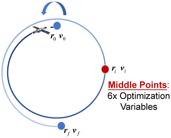
Figure 2. Connecting trajectories for computing multi-revolution transfers.

1.

Global Search: A particle swarm optimization (PSO) algorithm explores the high-dimensional optimization space $\{{\mathit{s}}_k,\Delta {\mathit{v}}_{\mathrm{launch}}\}$, minimizing $J+{\sum }_k{P}_{\mathrm{feas}}$.

2.

Local Refinement: The best candidate from PSO is passed to a gradient-based local solver [42] to fine-tune the intermediate states and launch velocity, further reducing the objective while strictly enforcing segment continuity and feasibility.

3. Results

Among the numerous near-Earth asteroid analyzed, three representative porkchop plots, corresponding to asteroids 2012 LA, 2008 ST, and 2022 OC3, are presented for demonstration. Their orbital elements are shown in Table 3 and Figure 3.

Table 3. Classical orbital elements of selected asteroids.

Epoch	Asteroid	a (km)	e	i (°)	$\mathbf{\Omega }$ (°)	$\mathit{\omega }$ (°)	$\mathit{\nu }$ (°)
2029 Jan 01 12:00:00 UTC	2012 LA	$1.55604\times {10}^8$	0.0216877	21.7262	353.0774	320.1778	257.0437
	2008 ST	$1.43986\times {10}^8$	0.1265623	21.5865	359.3513	120.5766	157.4352
	2022 OC3	$1.52899\times {10}^8$	0.1286078	22.9596	0.5957	49.6797	113.2483

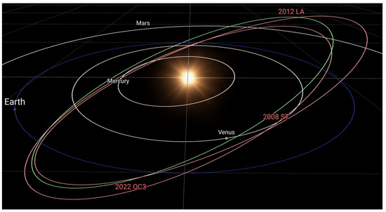
Figure 3. Orbits of selected asteroids. Credits: ESA NEO Toolkit.

The porkchop plots for these three asteroids are shown in Figure 4, Figure 5 and Figure 6. In each plot, the horizontal axis represents the launch date, the vertical axis represents the time of flight, and the color scale indicates fuel consumption. For comparison, the direct method results are compared with those from the neural network model. The direct method (numerical results) accounts for variable specific impulse, maximum thrust, and includes path constraints, whereas the neural network model (prediction results) is based on an indirect method using piece-wise variable specific impulse and maximum thrust. For asteroid 2012 LA, large regions of low fuel consumption appear in the porkchop plot, and the neural network model results closely match the direct method. The porkchop plot for asteroid 2008 ST exhibits a more complex structure, with multiple high fuel consumption regions, and significant discrepancies between the neural network model results and the direct method in some areas. The porkchop plot for asteroid 2022 OC3 exhibits even more pronounced discrepancies, as the optimal control direct method results display numerous discontinuities and gaps. The characteristics of these distinct porkchop plots will be discussed in detail in the following section.

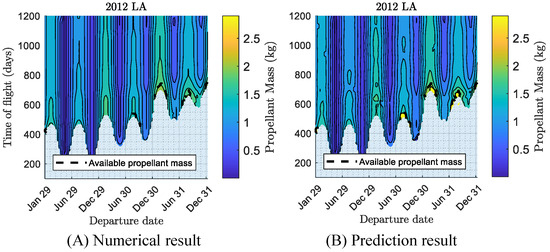
Figure 4. Porkchop plot for the 2012 LA Asteroid.

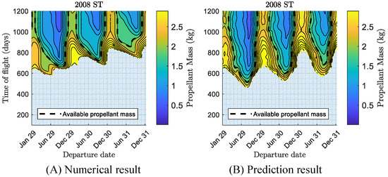
Figure 5. Porkchop plot for the 2008 ST Asteroid.

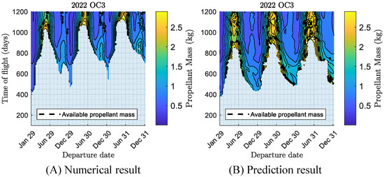
Figure 6. Porkchop plot for the 2022 OC3 Asteroid.

4. Analysis and Discussion

This section further investigates the causes of the non-negligible errors observed in the previous section. Intuitively, these errors may arise from the approximation inherent in the neural network model or from the complexity of the orbital dynamics and constraint. To isolate the effect of the neural network, variable specific impulse, thrust, and path constraints are removed in this experiment, leaving only the core dynamical model. The resulting relative error plots are shown in Figure 7, Figure 8 and Figure 9. As illustrated in the figures, the neural network consistently captures the overall trends and salient features of the trajectory across all asteroid scenarios. This demonstrates the model’s capability to represent the underlying orbital dynamics and validates the effectiveness of the proposed learning-based approach. The discrepancies between the porkchop plots and the neural network predictions for asteroid 2008 ST are further analyzed to investigate the underlying reasons for the observed differences. As shown in Figure 8, removing the constraints leads to significantly different porkchop plot structures compared to the original ones in Figure 5. This indicates that the new structures arise from the inclusion of variable specific impulse $I_{\mathrm{sp}}$, maximum thrust $T_{max}$, and path constraints specific to this scenario.

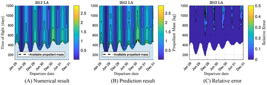
Figure 7. Porkchop plot for the Asteroid 2012 LA without variable $I_{\mathrm{sp}}$, $T_{max}$, and path constraints.

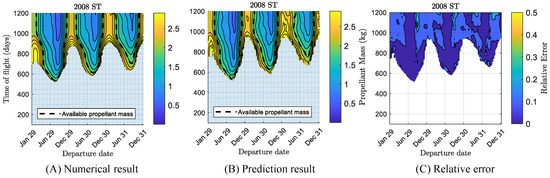
Figure 8. Porkchop plot for the Asteroid 2008 ST without variable $I_{\mathrm{sp}}$, $T_{max}$, and path constraints.

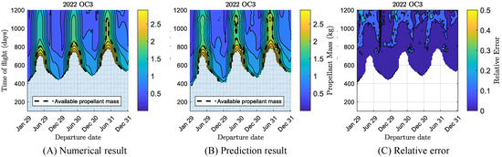
Figure 9. Porkchop plot for the Asteroid 2022 OC3 without variable $I_{\mathrm{sp}}$, $T_{max}$, and path constraints.

Therefore, the individual effects of variable specific impulse, maximum thrust, and path constraints on the porkchop plots are further investigated. To this end, porkchop plots with and without variable specific impulse, maximum thrust, and path constraints are generated using a direct method of optimal control, as shown in Figure 10. The variations in specific impulse and maximum thrust have a relatively minor impact on the orbital transfer, resulting in only slight structural changes in the porkchop plots. In contrast, the introduction of path constraints significantly affects the porkchop plot, particularly near its boundaries, and substantially alters the overall plot structure. This suggests that, in the later stages of mission planning, the influence of path constraints must be carefully accounted for to optimize launch window selection.

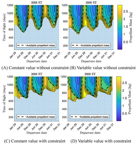
Figure 10. Comparison of porkchop plots with variable $I_{\mathrm{sp}}$, $T_{max}$ and path constraints by optimal control method.

Further analysis of the reverse-computed trajectories, shown in Figure 11, reveals that the optimal control method, constrained by path boundaries, produces trajectories that closely follow the 0.8 AU limit. In contrast, the neural network approach, which does not impose path constraints, results in infeasible trajectories in certain regions. This shows that at the point with the largest prediction error, there is a significant difference between subplots (d) and (e), which correspond to the path-constrained scenarios. This indicates that the current neural network model may produce large estimation errors when physical path constraints are present. This also highlights the need for future research to incorporate such constraints into the network model.

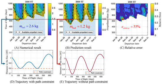
Figure 11. Porkchop plot for the 2008 ST Asteroid with path constraint.

In some cases, the presence of multiple local optima causes the optimal control method based on the solution-continuation technique to fail in capturing the complete global cost landscape, as illustrated in Figure 12. Although this issue can be mitigated through extensive trial runs, such an approach would inevitably lead to significantly increased computation time. This challenge becomes particularly pronounced when screening a large number of candidate asteroids for exploration, where the global computational burden becomes increasingly prohibitive. This scenario presents a compelling case for the use of neural network models. When trained on a sufficient amount of high-quality data, neural networks can leverage their global approximation capability to provide smooth and reasonable fuel consumption estimates. Moreover, due to their high computational efficiency, neural networks enable the use of global optimization algorithms within a reasonable time frame, even in scenarios requiring further optimization like tuning the launcher’s velocity in this paper’s study, making them a promising alternative.

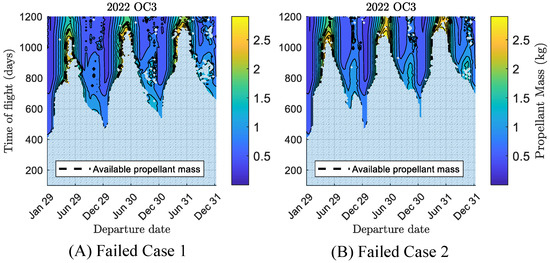
Figure 12. Example of failed cases of solution continuation with direct method, due to discontinuities in $I_{\mathrm{sp}}$, $T_{max}$.

5. Conclusions

This work presents a comparative study of the performance of optimal control methods and neural-network-based estimation approaches on porkchop plots, a widely adopted tool in mission analysis. In simple cases without path constraints, the neural network approach is able to reproduce the structural characteristics of the original porkchop plot while maintaining relative prediction errors below 10% in the majority of regions. In scenarios involving multiple local optima where continuation-based optimal control methods may fail, the neural network approach remains stable due to its independence from initial guesses. This facilitates efficient identification of asteroid targets with scientific or engineering value by mission designers. Currently, practical engineering constraints, such as path constraints, have not yet been incorporated into the neural network model, which limits its applicability in some cases. Future research could focus on integrating these constraints into the learning framework, or exploring approaches guided by physical constraints. This paper also presents a new perspective on the application of neural networks in astrodynamics. The generation of porkchop plots is inherently intuitive and easy to visualize, while enabling the validation and verification of a large number of orbital transfer scenarios, thus allowing for a straightforward assessment of prediction quality. More importantly, this tool is widely used in mission preliminary design and is particularly valuable in early-stage planning, where a higher tolerance for solution inaccuracy is often acceptable. The introduction of neural networks can significantly enhance the efficiency of mission designers. Furthermore, due to their independence from domain-specific expertise, planetary science teams can quickly perform preliminary filtering during the initial mission phase, thereby reducing communication and iteration costs, which offers practical value for engineering applications.

References

- Zhang, Z.; Zhang, N.; Guo, X.; Wu, D.; Xie, X.; Yang, J.; Jiang, F.; Baoyin, H. Sustainable Asteroid Mining: On the Design of GTOC12 Problem and Summary of Results. Astrodynamics 2025, 9, 3–17. [Google Scholar] [CrossRef]
- Granvik, M.; Morbidelli, A.; Jedicke, R.; Bolin, B.; Bottke, W.F.; Beshore, E.; Vokrouhlický, D.; Nesvorný, D.; Michel, P. Debiased Orbit and Absolute-Magnitude Distributions for near-Earth Objects. Icarus 2018, 312, 181–207. [Google Scholar] [CrossRef]
- Lauretta, D.S.; Balram-Knutson, S.S.; Beshore, E.; Boynton, W.V.; Drouet d’Aubigny, C.; DellaGiustina, D.N.; Enos, H.L.; Golish, D.R.; Hergenrother, C.W.; Howell, E.S.; et al. OSIRIS-REx: Sample Return from Asteroid (101955) Bennu. Space Sci. Rev. 2017, 212, 925–984. [Google Scholar] [CrossRef]
- Cheng, A.F.; Rivkin, A.S.; Michel, P.; Atchison, J.; Barnouin, O.; Benner, L.; Chabot, N.L.; Ernst, C.; Fahnestock, E.G.; Kueppers, M.; et al. AIDA DART Asteroid Deflection Test: Planetary Defense and Science Objectives. Planet. Space Sci. 2018, 157, 104–115. [Google Scholar] [CrossRef]
- Watanabe, S.i.; Tsuda, Y.; Yoshikawa, M.; Tanaka, S.; Saiki, T.; Nakazawa, S. Hayabusa2 Mission Overview. Space Sci. Rev. 2017, 208, 3–16. [Google Scholar] [CrossRef]
- Ferrari, F.; Franzese, V.; Pugliatti, M.; Giordano, C.; Topputo, F. Preliminary Mission Profile of Hera’s Milani CubeSat. Adv. Space Res. 2021, 67, 2010–2029. [Google Scholar] [CrossRef]
- Topputo, F.; Wang, Y.; Giordano, C.; Franzese, V.; Goldberg, H.; Perez-Lissi, F.; Walker, R. Envelop of Reachable Asteroids by M-ARGO CubeSat. Adv. Space Res. 2021, 67, 4193–4221. [Google Scholar] [CrossRef]
- Zhang, Z.; Guo, X.; Wu, D.; Baoyin, H.; Li, J.; Topputo, F. Global Optimality in Multi-Flyby Asteroid Trajectory Optimization: Theory and Application Techniques. arXiv 2025, arXiv:2508.02904. [Google Scholar] [CrossRef]
- Betts, J.T. Survey of Numerical Methods for Trajectory Optimization. J. Guid. Control. Dyn. 1998, 21, 193–207. [Google Scholar] [CrossRef]
- Dellnitz, M.; Ober-Blöbaum, S.; Post, M.; Schütze, O.; Thiere, B. A Multi-Objective Approach to the Design of Low Thrust Space Trajectories Using Optimal Control. Celest. Mech. Dyn. Astron. 2009, 105, 33–59. [Google Scholar] [CrossRef]
- Betts, J.T. Chapter 4: The Optimal Control Problem. In Practical Methods for Optimal Control Using Nonlinear Programming, 3rd ed.; Advances in Design and Control; Society for Industrial and Applied Mathematics: Philadelphia, PA, USA, 2020; pp. 115–212. [Google Scholar] [CrossRef]
- Zhang, Z.; Zhang, N.; Chen, Z.; Jiang, F.; Baoyin, H.; Li, J. Global Trajectory Optimization of Multispacecraft Successive Rendezvous Using Multitree Search. J. Guid. Control Dyn. 2024, 47, 503–517. [Google Scholar] [CrossRef]
- Malyuta, D.; Reynolds, T.P.; Szmuk, M.; Lew, T.; Bonalli, R.; Pavone, M.; Acikmese, B. Convex Optimization for Trajectory Generation. arXiv 2021, arXiv:2106.09125. [Google Scholar] [CrossRef]
- Yamaguchi, S.; Hiraiwa, N.; Bando, M.; Hokamoto, S.; Henry, D.B.; Scheeres, D.J. Trajectory design for awaiting comets on invariant manifolds with optimal control. Astrodynamics 2025, 9, 565–581. [Google Scholar] [CrossRef]
- Pavanello, Z.; Pirovano, L.; Armellin, R.; De Vittori, A.; Di Lizia, P. Collision avoidance maneuver optimization during low-thrust propelled trajectories. Astrodynamics 2025, 9, 247–271. [Google Scholar] [CrossRef]
- Jiang, F.; Baoyin, H.; Li, J. Practical Techniques for Low-Thrust Trajectory Optimization with Homotopic Approach. J. Guid. Control Dyn. 2012, 35, 245–258. [Google Scholar] [CrossRef]
- Bertrand, R.; Epenoy, R. New Smoothing Techniques for Solving Bang–Bang Optimal Control Problems—Numerical Results and Statistical Interpretation. Optim. Control. Appl. Methods 2002, 23, 171–197. [Google Scholar] [CrossRef]
- Morelli, A.C.; Hofmann, C.; Topputo, F. Robust Low-Thrust Trajectory Optimization Using Convex Programming and a Homotopic Approach. IEEE Trans. Aerosp. Electron. Syst. 2022, 58, 2103–2116. [Google Scholar] [CrossRef]
- Acciarini, G.; Beauregard, L.; Izzo, D. Computing Low-Thrust Transfers in the Asteroid Belt, a Comparison between Astrodynamical Manipulations and a Machine Learning Approach. arXiv 2024, arXiv:2405.18918. [Google Scholar] [CrossRef]
- Zhu, Y.h.; Luo, Y.Z. Fast Evaluation of Low-Thrust Transfers via Multilayer Perceptions. J. Guid. Control Dyn. 2019, 42, 2627–2637. [Google Scholar] [CrossRef]
- Li, H.; Chen, S.; Izzo, D.; Baoyin, H. Deep Networks as Approximators of Optimal Low-Thrust and Multi-Impulse Cost in Multitarget Missions. Acta Astronaut. 2020, 166, 469–481. [Google Scholar] [CrossRef]
- Yang, J.; Zhang, Z.; Li, J.; Jiang, F. Deep Neural Networks-Based Efficient Mapping of Three-Dimensional Lunar Gravity Assist in the Circular Restricted Three-Body Problem. IEEE Trans. Aerosp. Electron. Syst. 2025, 61, 10768–10783. [Google Scholar] [CrossRef]
- Singh, S.K.; Junkins, J.L. Stochastic learning and extremal-field map based autonomous guidance of low-thrust spacecraft. Sci. Rep. 2022, 12, 17774. [Google Scholar] [CrossRef]
- Kim, I.; Singh, S. Probabilistic regression for autonomous terrain relative navigation via multi-modal feature learning. Sci. Rep. 2024, 14, 29966. [Google Scholar] [CrossRef]
- Mancini, P.; Cannici, M.; Matteucci, M. Deep learning for asteroids autonomous terrain relative navigation. Adv. Space Res. 2023, 71, 3748–3760. [Google Scholar] [CrossRef]
- Sánchez-Sánchez, C.; Izzo, D. Real-Time Optimal Control via Deep Neural Networks: Study on Landing Problems. J. Guid. Control Dyn. 2018, 41, 1122–1135. [Google Scholar] [CrossRef]
- Izzo, D.; Öztürk, E. Real-Time Guidance for Low-Thrust Transfers Using Deep Neural Networks. J. Guid. Control Dyn. 2021, 44, 315–327. [Google Scholar] [CrossRef]
- Lunghi, P.; Silvestrini, S.; Dold, D.; Meoni, G.; Hadjiivanov, A.; Izzo, D. Energy efficiency analysis of Spiking Neural Networks for space applications. Astrodynamics 2025, 9, 909–932. [Google Scholar] [CrossRef]
- Smith, T.K.; Akagi, J.; Droge, G. Model predictive control for formation flying based on D’Amico relative orbital elements. Astrodynamics 2025, 9, 143–163. [Google Scholar] [CrossRef]
- Hornik, K.; Stinchcombe, M.; White, H. Multilayer Feedforward Networks Are Universal Approximators. Neural Netw. 1989, 2, 359–366. [Google Scholar] [CrossRef]
- Sidhoum, Y.; Oguri, K. Pontryagin-Bellman Differential Dynamic Programming for Low-Thrust Trajectory Optimization with Path Constraints. arXiv 2025, arXiv:2502.20291. [Google Scholar]
- D’Ambrosio, A.; Benedikter, B.; Furfaro, R. Physics-Informed Pontryagin Neural Networks for Path-Constrained Optimal Control Problems. J. Guid. Control Dyn. 2025, 48, 8. [Google Scholar] [CrossRef]
- Domahidi, A.; Chu, E.; Boyd, S. ECOS: An SOCP solver for embedded systems. In Proceedings of the 2013 European Control Conference (ECC), Zurich, Switzerland, 17–19 July 2013. [Google Scholar]
- Topputo, F.; Zhang, C. Survey of Direct Transcription for Low-Thrust Space Trajectory Optimization with Applications. Abstr. Appl. Anal. 2014, 2014, 851720. [Google Scholar] [CrossRef]
- Morelli, A.C.; Mannocchi, A.; Giordano, C.; Ferrari, F.; Topputo, F. Initial Trajectory Assessment of a low-thrust option for the RAMSES Mission to (99942) Apophis. Adv. Space Res. 2024, 73, 4241–4253. [Google Scholar] [CrossRef]
- Taheri, E.; Abdelkhalik, O. Initial three-dimensional low-thrust trajectory design. Adv. Space Res. 2016, 57, 889–903. [Google Scholar] [CrossRef]
- Narayanaswamy, S.; Damaren, C.J. Equinoctial Lyapunov Control Law for Low-Thrust Rendezvous. J. Guid. Control Dyn. 2023, 46, 781–795. [Google Scholar] [CrossRef]
- Walker, M.J.H.; Ireland, B.; Owens, J. A Set Modified Equinoctial Orbit Elements. Celest. Mech. 1985, 36, 409–419. [Google Scholar] [CrossRef]
- Junkins, J.L.; Taheri, E. Exploration of Alternative State Vector Choices for Low-Thrust Trajectory Optimization. J. Guid. Control Dyn. 2019, 42, 47–64. [Google Scholar] [CrossRef]
- Gao, Y.; Kluever, C. Low-Thrust Interplanetary Orbit Transfers Using Hybrid Trajectory Optimization Method with Multiple Shooting. In AIAA/AAS Astrodynamics Specialist Conference and Exhibit; Guidance, Navigation, and Control and Co-located Conferences; American Institute of Aeronautics and Astronautics: Reston, VA, USA, 2004. [Google Scholar] [CrossRef]
- Zhang, Z.; Topputo, F. Neural Approximators for Low-Thrust Trajectory Transfer Cost and Reachability. arXiv 2025, arXiv:2508.02911. [Google Scholar] [CrossRef]
- Johnson, S.G. The Nlopt Nonlinear-Optimization Package. 2014. Available online: http://github.com/stevengj/nlopt (accessed on 1 January 2024).
Disclaimer/Publisher’s Note: The statements, opinions and data contained in all publications are solely those of the individual author(s) and contributor(s) and not of MDPI and/or the editor(s). MDPI and/or the editor(s) disclaim responsibility for any injury to people or property resulting from any ideas, methods, instructions or products referred to in the content. |
© 2026 by the authors. Licensee MDPI, Basel, Switzerland. This article is an open access article distributed under the terms and conditions of the Creative Commons Attribution (CC BY) license.