Role of Interfacial Dzyaloshinskii–Moriya Interactions on Dipole-Exchange Spin Waves in Finite-Width Ferromagnetic Nanostripes

Abstract

In this paper, we explore the magnetization dynamics in a long ferromagnetic nanostripe with finite width in the presence of antisymmetric Dzyaloshinskii–Moriya exchange interactions (DMIs). It is known that DMIs, which are currently of great interest because they give rise to chiral and nonreciprocal properties and influence surface topologies, can be enhanced by interfacing the nanostripe with a heavy metal. Our theoretical approach employs a microscopic (or Hamiltonian-based) analysis that includes symmetric bilinear exchange, antisymmetric DMI, long-range dipole–dipole interactions, and Zeeman energy due to an external magnetic field applied out of the plane of the nanostripe. In this geometry, we calculate the frequencies and amplitudes of the discrete spin-wave modes that have a standing-wave character across the finite width of the stripe and a propagating character (with wavenumber k) along the stripe length. The individual spin-wave modes display nonreciprocal propagation in their dispersion relations due to DMI. We also find that there may be localized edge spin waves with amplitudes that undergo spatial decay near the stripe edges.

1. Introduction

The concept of antisymmetric exchange interaction in magnetic materials was introduced several decades ago by Dzyaloshinskii [1,2] and Moriya [3]. Soon afterward, this extra interaction was found [4] to well account for the spin waves in canted antiferromagnet FeBO₃ and other rhombohedral materials. Also, it was pointed out by Melcher [5] that Dzyaloshinskii–Moriya interactions (or DMIs) would give rise to a term in the spin-wave (SW) dispersion of ferromagnets that is linear in the wave vector. However, it was found that DMI generally provided a rather small effect on the magnetization dynamics.

More recently, this situation was dramatically changed with the discovery of interfacial Dzyaloshinskii–Moriya interactions (or DMIs) in thin films and magnetic nanostructures. This occurs when there is an interface between a ferromagnetic or antiferromagnetic material and certain heavy metals (for example, Fe/Ir and Mn/W bilayers). The pronounced enhancement of DMI in such circumstances has revitalized the interest in DMI as it pertains to the static properties and magnetization dynamics of magnetic materials, especially in confined geometries and nanostructures (see, e.g., [6,7,8,9,10,11] for general references). The literature dedicated to the diverse aspects of DMI is now very extensive, with much of it driven by the potential for applications in signal processing [11,12], magnetic memories [13,14], magnetic logic devices [15,16,17], spintronics [18,19,20,21], chiral magnonics [13,22,23,24], domain walls [11,25,26,27], and spin textures such as skyrmions [11,13].

From a more fundamental perspective, the role of DMI in modifying the properties of the SW modes has received a great deal of attention. The first reported measurement of nonreciprocal SW propagation in thin films due to interfacial DMI was made by Zakeri et al. [6,28] using spin-polarized electron energy-loss spectroscopy (SPEELS) for an ultrathin Fe/W sample. Other studies soon followed for different magnetic materials and/or techniques including Brillouin light scattering (BLS) and ferromagnetic resonance (FMR) (see, for example, [8,9,29,30,31,32,33,34] for thin films). On the theoretical side, Kostylev [35] investigated the interface boundary conditions and SW dynamics for a ferromagnetic film with DMI.

There are relatively fewer works on nanostripes (either individually or in arrays) with DMI, since the lateral edges need to be taken into account in any analysis. We comment on some notable references below [36,37,38,39,40]. All of these cases refer to studies in which the static magnetization lies in the plane of the stripe, corresponding to either the geometry for Damon–Eshbach (DE) modes or backward volume (BV) modes. In [37], BLS measurements were reported, while in [36], simulations were conducted that applied the zero-wave-vector modes occurring in FMR. In Silvani et al. [38], a simulation package was employed to study the frequencies and eigenvectors for SWs in the BV configuration. In simulations conducted by Gallardo et al. [39,40], channeling effects were explored for SWs in stripes with a lateral compositional grading.

Our focus in this work is to develop a theoretical study on the effect of interfacial DMI on SW modes in ferromagnetic nanowires taking the form of finite-width nanostripes. In contrast to the aforementioned works on stripes, we consider a different geometry, namely, the forward volume (FV) configuration, in which the static magnetization is perpendicular to the plane of the stripe. Also, we use a different methodology, based on a microscopic (or Hamiltonian-based) approach with the dipole–dipole interactions and bilinear exchange interactions included along with the DMI terms. We are motivated to explore the possibilities for SW quantization effects in the lateral (or width) direction and to study SW localization, particularly at the lateral edges. Already, this well-established approach has been successfully employed in analogous studies (including comparisons with BLS and FMR measurements) for nanowires and nanostripes in the absence of DMI (see, e.g., [41,42,43,44,45]). With this technique, the nanostripe is represented by an array of small cells (each with an effective spin) and the quantum-mechanical operator equations of motion are used to deduce the SW spectra. In the present context, this method has advantages compared with employing the alternative continuum methods based on the Landau–Lifschitz–Gilbert (LLG) torque equation (see, e.g., [46,47,48,49]), because we will be studying SWs at large wave vectors (implying short wavelengths).

The paper is organized as follows. In Section 2, we present the geometry and scheme of magnetic interactions for the nanostripes. Here, the theory is developed by focusing initially on the exchange-dominated case with competing effects between the symmetric bilinear terms and the antisymmetric DMI. Then, generalization to include the role of magnetic dipole–dipole interactions is described. The results of our analysis are given in Section 3, where we emphasize the SW dispersion relations, illustrating the nonreciprocity in SW propagation due to DMI and the existence of localized SW modes. Results are also given for the spatial variation in the SW amplitudes across the width of the nanostripes. Additional discussion and conclusions are presented in Section 4.

2. Materials and Methods

The setup under consideration consists of a ferromagnetic wire in the form of a nanostripe located in the $xy$-plane with an infinite length along the y direction and a finite width W in the x direction. We assume that the externally applied magnetic field $B_0$ acts along the z direction, which is out of the plane of the nanostripe. We divide the stripe volume up into cells (which are cuboids of sides $a\times a\times a$), as depicted in Figure 1. The label n is used to enumerate the cells across the width and each cell contains an effective spin or magnetic moment. The criterion for how small the cell size should be taken in an inhomogeneously magnetized sample is well known from micromagnetics (see, e.g., [49,50,51]). The requirement is that a should be chosen to be comparable with or smaller than the so-called exchange correlation length $a_{ex}$, which is typically several nm in a metallic material (e.g., $a_{ex}\sim 6$ nm in permalloy). The stripe is assumed to be interfaced with a heavy (nonmagnetic) metal that serves to provide an interfacial DMI.

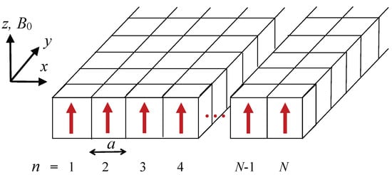
Figure 1. Geometry for a finite-width ferromagnetic stripe, where the individual cubic cells have sides of length a. There are N cells (labeled with row number n) across the width where $W=Na$. The applied field $B_0$ is along the z direction.

First, we describe the total effective spin Hamiltonian $\mathcal{H}$ for the system, in which we include the competing magnetic effects due to the symmetric bilinear exchange interactions, the antisymmetric DMI terms, the long-range magnetic dipole–dipole interactions, and the Zeeman energy of the applied field $B_0$. The spin operators ${\mathbf{S}}_{nl}$ associated with each magnetic cell are specified by the row number n ($=1,2,\dots ,N$) across the width (x direction) and label l for the coordinate along the infinite length (y direction). We may write

$$\begin{array}{ccc}\hfill \mathcal{H}& =& -{\displaystyle \frac{1}{2}}\sum _{nl,mj}{J}_{nl,mj}{\mathbf{S}}_{nl}·{\mathbf{S}}_{mj}-{\displaystyle \frac{1}{2}}\sum _{nl,mj}{\mathbf{J}}_{\mathit{nl},\mathit{mj}}^{DM}·({\mathbf{S}}_{nl}\times {\mathbf{S}}_{mj})\hfill \\ & & +{\displaystyle \frac{1}{2}}{\left(g{\mu }_B\right)}^2\sum _{nl,mj}\sum _{\alpha ,\beta }{D}_{nl,mj}^{\alpha \beta }{S}_{nl}^{\alpha }{S}_{mj}^{\beta }-g{\mu }_B{B}_0\sum _{nl}{S}_{nl}^z.\hfill \end{array}$$

(1)

Here, $J_{nl,mj}$ and ${\mathbf{J}}_{nl,mj}^{DM}$ are the scalar bilinear exchange coefficient and the vector DMI exchange coefficient, respectively. Typically, they are of short range, and we assume in this work that they are nonzero only between nearest-neighbour spins. They may, however, be perturbed at the lateral edges of the stripe if the electronic wave functions are modified due to the local lowering of symmetry. For convenience in this work, we take the case where the DMI axis is along the z direction by writing ${\mathbf{J}}_{\mathit{nl},\mathit{mj}}^{DM}=\widehat{\mathbf{z}}{J}_{nl,mj}^{DM}$ with $\widehat{\mathbf{z}}$ denoting a unit vector. Hence, the DMI term in the Hamiltonian involves $\widehat{\mathbf{z}}·({\mathbf{S}}_{nl}\times {\mathbf{S}}_{mj})=S_{nl}^x{S}_{mj}^y-S_{nl}^y{S}_{mj}^x.$

In the next term of the Hamiltonian, we denote the coefficients of the magnetic dipole–dipole interaction from electromagnetism as $D_{nl,mj}^{\alpha \beta }$ (see, e.g., [48,52]), where

$$\begin{array}{ccc}\hfill D_{nl,mj}^{\alpha \beta }& =& {\displaystyle \frac{|{\mathbf{r}}_{nl,mj}{|}^2{\delta }_{\alpha \beta }-3r_{nl,mj}^{\alpha }{r}_{nl,mj}^{\beta }}{|{\mathbf{r}}_{nl,mj}{|}^5}},\hfill \end{array}$$

(2)

expressing g and ${\mu }_B$ as the Landé factor and Bohr magneton, respectively. The superscripts $\alpha$ and $\beta$ represent Cartesian components x, y, or z, and ${\mathbf{r}}_{nl,mj}$ is the vector joining the pair of sites. The final term in Equation (1) represents the Zeeman field energy.

The first step in the analysis is to investigate the equilibrium spin directions. In the absence of DMI, the spin orientations are stabilized to be along the z direction by a static field $B_0$ that is sufficient to overcome the shape demagnetizing effects from the dipole–dipole terms. A standard procedure, analogous to the mean-field approach used (for example) in [42,53,54], is to write down the total energy functional $\overline{E}$ deduced from the above Hamiltonian by replacing each quantum-mechanical spin operator with its corresponding classical vector ${\overline{\mathbf{S}}}_{nl}\equiv ({\overline{S^x}}_{nl},{\overline{S^y}}_{nl},{\overline{S^z}}_{nl})$. The Cartesian components of the static effective magnetic field can then be obtained from the derivative

$$\begin{array}{ccc}\hfill {\overline{B^{\alpha }}}_n& =& -{\displaystyle \frac{1}{g{\mu }_B}}{\displaystyle \frac{𝜕\overline{E}}{𝜕{\overline{S^{\alpha }}}_{nl}}},(\alpha =x,y,z).\hfill \end{array}$$

(3)

The subscript l has been dropped on the left-hand side because all cells in row n are equivalent by symmetry in the mean-field theory. We find

$$\begin{array}{ccc}\hfill g{\mu }_B{\overline{B}}_n^x& =& \sum _{mj}\left\{J_{nl,mj}{\overline{S}}_{mj}^x+J_{nl,mj}^{DM}{\overline{S}}_{mj}^y+{\left(g{\mu }_B\right)}^2\left(D_{nl,mj}^{xx}{\overline{S}}_{mj}^x+D_{nl,mj}^{xy}{\overline{S}}_{mj}^y\right)\right\},\hfill \\ \hfill g{\mu }_B{\overline{B}}_n^y& =& \sum _{mj}\left\{J_{nl,mj}{\overline{S}}_{mj}^y-J_{nl,mj}^{DM}{\overline{S}}_{mj}^x+{\left(g{\mu }_B\right)}^2\left(D_{nl,mj}^{yy}{\overline{S}}_{mj}^y+D_{nl,mj}^{xy}{\overline{S}}_{mj}^x\right)\right\},\hfill \\ \hfill g{\mu }_B{\overline{B}}_n^z& =& g{\mu }_B{B}_0+\sum _{mj}\left\{J_{nl,mj}{\overline{S}}_{mj}^z+{\left(g{\mu }_B\right)}^2{D}_{nl,mj}^{zz}{\overline{S}}_{mj}^z\right\}.\hfill \end{array}$$

(4)

A close inspection of these equations shows that the transverse components $B_n^x$ and $B_n^y$ of the effective field do not couple to any longitudinal (or z) spin components, whereas $B_n^z$ couples only to z spin components. Ultimately, it follows that there is no tilting of the spins away from the z direction for their equilibrium orientations. This is actually a special property found when taking the DMI axis to be along the z direction, as we mention later in Section 4.

2.1. SW Formalism in the Exchange-Dominated Case

To illustrate the methodology involved in calculating the SW spectrum of the nanostripes with edge effects incorporated, it is convenient to start with a case in which the exchange interactions (bilinear and DMI) dominate over the dipole–dipole interactions. We take the parameters for the bilinear and DMI exchange between nearest neighbours to be of magnitude J and $J^{DM}$, respectively, and zero otherwise. Additionally, we allow for the possibility of modifications in the bilinear exchange at the two lateral edges by denoting the nearest-neighbour exchange parameter as $J_E$. The general case with dipolar effects included will be presented in a later section.

To proceed we introduce the Holstein–Primakoff transformation [55] from spin operators to boson creation $a_{nl}^{†}$ and annihilation $a_{nl}$ operators (see also [47,48,52,56]). Denoting the spin raising and lowering operators by $S_{nl}^{\pm }=S_{nl}^x\pm i{S}_{nl}^y,$ we have at temperatures well below the Curie temperature $T_C$

$$\begin{array}{ccc}\hfill S_{nl}^{+}& =& \sqrt{2S}\left(a_{nl}-{\displaystyle \frac{1}{4S}}{a}_{nl}^{†}{a}_{nl}{a}_{nl}+\dots \right),\hfill \end{array}$$

(5)

while $S_{nl}^{-}$ denotes its Hermitian conjugate and $S_{nl}^z=S-a_{nl}^{†}{a}_{nl}$. After making the transformation, the Hamiltonian in Equation (1) can be expanded in the form $\mathcal{H}=E_0+{\mathcal{H}}^{\left(1\right)}+{\mathcal{H}}^{\left(2\right)}+{\mathcal{H}}^{\left(3\right)}+\dots ,$ where any general term written as ${\mathcal{H}}^{\left(p\right)}$ involves a product of p creation or annihilation operators. Here, $E_0$ is a scalar constant which has no effect on the SW dynamics, the term ${\mathcal{H}}^{\left(1\right)}$ is found to vanish identically by symmetry, and so the linearized SW spectrum at low temperatures is given by the leading-order operator term ${\mathcal{H}}^{\left(2\right)}$. The next terms in the expansion describe interaction processes of higher order between the SWs, and will be neglected in the present study.

The translational symmetry of the nanostripes along the length direction (the y axis) can next be utilized to make a Fourier transform to wave–vector component k while retaining the row label n to specify the position across the finite width. The Hamiltonian term ${\mathcal{H}}^{\left(2\right)}$ then has the general bilinear form

$$\begin{array}{ccc}\hfill {\mathcal{H}}^{\left(2\right)}& =& \sum _k\sum _{n,m}{A}_{n,m}\left(k\right)a_{k,n}^{†}{a}_{k,m}.\hfill \end{array}$$

(6)

Here, the operators have been expressed in a “mixed” representation with labels like $\{k,n\}$. The coefficients $A_{n,m}\left(k\right)$ can be regarded as the elements of a finite $N\times N$ matrix $\mathit{A}$ defined by

$$\begin{array}{ccc}\hfill \mathit{A}& =& SJ\left(\begin{array}{ccccc}{c}_0& -1+i\alpha & 0& 0& \dots \\ -1-i\alpha & c& -1+i\alpha & 0& \dots \\ 0& -1-i\alpha & c& -1+i\alpha & \dots \\ 0& 0& -1-i\alpha & c& \dots \\ ⋮& ⋮& ⋮& ⋮& \ddots & ⋮& ⋮\\ & & & & \dots & c& -1+i\alpha \\ & & & & \dots & -1-i\alpha & c_0\end{array}\right),\hfill \end{array}$$

(7)

where we have defined a parameter for the relative strength of the DMI by $\alpha =J^{DM}/J$. The other quantities $c_0$ (which incorporates the edge effects) and c (which depends only on the bulk parameters) are defined as

$$\begin{array}{ccc}{c}_0\hfill & =\hfill & \left({\displaystyle \frac{g{\mu }_B{B}_0}{SJ}}\right)-2{\displaystyle \frac{J_E}{J}}cos\left(ka\right)-2\alpha sin\left(ka\right)+1+2{\displaystyle \frac{J_E}{J}},\hfill \end{array}$$

(8)

$$\begin{array}{ccc}c\hfill & =& \left({\displaystyle \frac{g{\mu }_B{B}_0}{SJ}}\right)-2cos\left(ka\right)-2\alpha sin\left(ka\right)+4.\hfill \end{array}$$

(9)

If the matrix in Equation (7) is diagonalized to obtain the eigenvalues and eigenvectors, we may deduce the SW energies and the corresponding spatial amplitudes of each mode. In general, this can be conducted numerically, as we describe later. However, analytic results can be found in some special cases by employing the property that $\mathit{A}$ is a tridiagonal matrix, i.e., it has nonzero elements only along the leading diagonal and the two diagonals on either side, allowing it to be solved analytically (see, e.g., [57]).

As an example of the analytic approach, we consider the semi-infinite limit of a wide stripe for which we look at the edge effects localized near $n=1$. The SW energies E are deduced as the eigenvalues of the matrix equation $\left(E\mathit{I}-\mathit{A}\right)\mathit{u}=\mathbf{0}$, where the eigenvector $\mathit{u}$ is a column matrix with elements $u_n$ ($n=1,2,3,\dots )$ representing SW amplitude factors. Multiplying the matrices row-by-row then yields the following set of coupled equations

$$\begin{array}{ccc}\hfill (E/SJ-c_0)u_1+(1-i\alpha )u_2& =& 0(\mathrm{row}1),\hfill \end{array}$$

(10)

$$\begin{array}{ccc}\hfill (1+i\alpha )u_{n-1}+(E/SJ-c)u_n+(1-i\alpha )u_{n+1}& =& 0(\mathrm{row}n>1).\hfill \end{array}$$

(11)

These equations have “bulk” SW solutions found by substituting $u_n\propto exp(-iqna)$ into Equation (11), where q is real giving a wave-like behaviour in the width direction x. After rearrangement, we find $E=SJc+2SJ[1-cos\left(qa\right)]+2J^{DM}sin\left(qa\right)$. This result corresponds to a bulk SW band, as we will discuss in Section 3.1.

In contrast, we may also seek attenuating solution of Equations (10) and (11) by considering $u_n$ to vary with n like $exp(-\lambda na)$. Here, $\lambda$ may be a complex quantity, provided Re$\left(\lambda \right)>0$ as a condition for localization. It is straightforward to show that

$$|exp(-\lambda a)|={\displaystyle \frac{{(1+{\alpha }^2)}^{1/2}}{3-2(J_E/J)+2cos\left(ka\right)[(J_E/J)-1]}}<1$$

(12)

for localized edge modes, depending on $\alpha$, $J_E/J$, and $ka$. For example, we conclude that no edge modes can exist when $J_E/J=1$ or when $ka=0$; however, when $ka=\pi /2$ (for example) the condition can be satisfied when either $J_E<J$ or $J_E>2J$, depending on $\alpha .$ These conditions correspond to either acoustic- or optic-type modes, respectively (see later in Section 3.1).

2.2. Inclusion of Dipole–Dipole Interactions

Next, we generalize the previous SW results to include the effects of dipole–dipole interactions. The theoretical approach that we follow is broadly analogous to the methodology used in [41,42,45,58] for other models and structures. Corresponding to the nanostripe geometry and our choice of coordinate axes (see Figure 1), the only nonzero dipole–dipole sums are those of the form $D^{xx}$, $D^{yy}$, $D^{zz}$, and $D^{xy}$. When the dipolar part ${\mathcal{H}}_{dip}$ of the total spin Hamiltonian in Equation (1) is transformed to boson creation and annihilation operators, and a Fourier transform to wave vector k is created as before, we eventually find that for the bilinear part

$$\begin{array}{ccc}\hfill H_{dip}^{\left(2\right)}& =& {\displaystyle \frac{1}{2}}S{\left(g{\mu }_B\right)}^2\sum _k\sum _{n,m}\{-D_{n,m}^{zz}\left(k\right)a_{k,n}^{†}{a}_{k,m}-2D_{n,m}^{z,z}\left(0\right)a_{k,n}^{†}{a}_{k,n}+{\displaystyle \frac{1}{2}}[D_{n,m}^{xx}\left(k\right)-D_{n,m}^{yy}\left(k\right)\hfill \\ & & +2i{D}_{n,m}^{xy}\left(k\right)]a_{k,n}^{†}{a}_{-k,m}^{†}+{\displaystyle \frac{1}{2}}\left[D_{n,m}^{xx}\left(k\right)-D_{n,m}^{yy}\left(k\right)-2i{D}_{n,m}^{xy}\left(k\right)\right]a_{k,n}{a}_{-k,m}\},\hfill \end{array}$$

(13)

In addition to the $a_{k,n}^{†}{a}_{k,m}$ terms found before in Equation (6) for the exchange-dominated case, we see that there are terms proportional to $a_{k,n}^{†}{a}_{-k,m}^{†}$ and $a_{k,n}{a}_{-k,m}$ that are dipolar in origin. Hence, we find that Equation (6) generalizes to become

$$\begin{array}{ccc}\hfill {\mathcal{H}}^{\left(2\right)}& =& \sum _k\sum _{n,m}\left\{A_{n,m}\left(k\right)a_{k,n}^{†}{a}_{k,m}+B_{n,m}\left(k\right)a_{k,n}^{†}{a}_{-k,m}^{†}+B_{n,m}^{*}\left(k\right)a_{k,n}{a}_{-k,m}\right\},\hfill \end{array}$$

(14)

where the A and B coefficients are defined below. First, the diagonal matrix elements $A_{n,n}\left(k\right)$ are

$$\begin{array}{ccc}\hfill A_{1,1}\left(k\right)& =& SJ{c}_0-S{\left(g{\mu }_B\right)}^2\sum _p{D}_{1,p}^{zz}\left(0\right)-{\displaystyle \frac{1}{2}}S{\left(g{\mu }_B\right)}^2{D}_{1,1}^{zz}\left(k\right)(n=1),\hfill \\ \hfill A_{n,n}\left(k\right)& =& SJc-S{\left(g{\mu }_B\right)}^2\sum _p{D}_{n,p}^{zz}\left(0\right)-{\displaystyle \frac{1}{2}}S{\left(g{\mu }_B\right)}^2{D}_{n,n}^{zz}\left(k\right)(1<n<N),\hfill \\ \hfill A_{N,N}\left(k\right)& =& SJ{c}_0-S{\left(g{\mu }_B\right)}^2\sum _p{D}_{N,p}^{zz}\left(0\right)-{\displaystyle \frac{1}{2}}S{\left(g{\mu }_B\right)}^2{D}_{N,N}^{zz}\left(k\right)(n=N),\hfill \end{array}$$

(15)

where the extra index p is summed from 1 to N. Next, all the off-diagonal elements of $A_{n,m}\left(k\right)$ have the additional dipolar term $-{\displaystyle \frac{1}{2}}S{\left(g{\mu }_B\right)}^2{D}_{n,m}^{zz}\left(k\right)$ compared with Equation (6). For the matrix elements $B_{n,m}\left(k\right)$ we have

$$\begin{array}{ccc}\hfill B_{n,m}\left(k\right)& =& {\displaystyle \frac{1}{4}}S{\left(g{\mu }_B\right)}^2\left[D_{n,m}^{xx}\left(k\right)-D_{n,m}^{yy}\left(k\right)+2i{D}_{n,m}^{xy}\left(k\right)\right].\hfill \end{array}$$

(16)

Finally, the bilinear Hamiltonian in Equation (14) can be diagonalized by applying a Bogoliubov-type linear transformation to a new set of boson operators $\left\{b_{k,\mathcal{l}}^{†}\right\}$ and $\left\{b_{k,\mathcal{l}}\right\}$ such that

$$\begin{array}{ccc}\hfill {\mathcal{H}}^{\left(2\right)}& =& \sum _{k,\mathcal{l}}{E}_{\mathcal{l}}\left(k\right)b_{k,\mathcal{l}}^{†}{b}_{k,\mathcal{l}}.\hfill \end{array}$$

(17)

This has the form of a sum over a discrete set of harmonic oscillators with energies $E_{\mathcal{l}}\left(k\right)$, where ℓ ($=1,2,\dots ,N$) is an SW mode number. The mathematical steps for carrying out the above procedure follows that used, for example, in [42,52,58]. The process leads to a $2N\times 2N$ block dynamical matrix given by

$$\left(\begin{array}{cc}\mathbf{A}\left(k\right)& 2\mathbf{B}\left(k\right)\\ -2{\mathbf{B}}^{*}\left(k\right)& -\tilde{\mathbf{A}}\left(k\right)\end{array}\right),$$

(18)

where the tilde denotes a matrix transpose. The N positive eigenvalues of the above matrix correspond to the physical SW modes of the system; there is another set of degenerate frequencies formed by the negative eigenvalues corresponding to the opposite sense of spin precession. Further, the components of the eigenvectors of the dynamical matrix provide the spatial amplitudes associated with any particular SW. They may be complex quantities in general, giving both a magnitude for the SW oscillation at that position and a relative phase.

3. Results

Here, we present numerical examples for the SW properties in finite-width nanostripes to illustrate the formal results derived in the previous section. We focus initially on the SW dispersion relations by showing the SW energy branches plotted versus the longitudinal wave vector k, illustrating bulk bands and localized edge modes as well as the important nonreciprocal propagation characteristic due to the DMI.

3.1. Exchange-Dominated Case

As in Section 2, we start with the limiting case when the exchange interactions (bilinear and DMI) dominate over effects due to the dipole–dipole interactions. In Figure 2, we show SW dispersion relations for a nanostripe with width corresponding to $N=12,$ taking the case of no perturbation to the edge bilinear exchange ($J_E=J$). The $ka$ values span the entire 1D Brillouin zone from $-\pi$ to $\pi$. The two plots correspond to (a) no DMI ($\alpha \equiv J^{DM}/J=0)$ and (b) nonzero DMI with $\alpha =0.3$. In the first case, the SW branches are symmetric between positive and negative $ka$, but this is not the case when DMI is present. It can be seen in the latter case that there exists expected nonreciprocal mode propagation associated with the DMI; the dispersion has become asymmetric in shape between positive and negative k with the minimum occurring at about $ka=0.3$ in this example. In both cases, it can be seen that there are 12 discrete SWs (the same number as N) representing standing modes across the width of the nanostripe. The applied magnetic field, both here and in our later examples, is chosen to satisfy $g{\mu }_B{B}_0/SJ=0.4$.

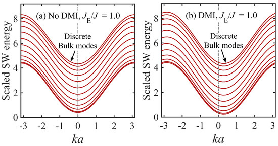
Figure 2. Dispersion relations for the discrete spin-wave (SW) modes in a ferromagnetic nanostripe with width parameter $N=12$ for the case where the exchange interactions dominate over the dipole–dipole interaction effects. The SW energies in units of $SJ$ are shown with and without Dzyaloshinskii–Moriya interactions (DMI) by taking (a) $\alpha =0$ and (b) $\alpha =0.3$. It is assumed that $J_E/J=1$.0, so there are no edge exchange perturbations here.

Next, in Figure 3 and Figure 4, we explore the effects of varying the edge exchange ratio $J_E/J$. We recall that in Section 2.1 an analysis was given indicating that (for wide stripes, at least) localized edge modes could exist for some parameter values, namely for $J_E<J$ or $J_E>2J$ when k is half of the Brillouin zone boundary value, namely, $ka=\pi /2$, depending on the $\alpha$ value. Thus, results for $J_E/J=0.2$ are shown in Figure 3a,b for no DMI ($\alpha =0$) and with DMI included ($\alpha =0.3$), respectively. The striking feature here, compared with the previous example, is that two SW modes that are almost degenerate in energy are split off from the band of bulk-like (or standing modes). These two modes, which occur over a wide range of k in the Brillouin zone, are the edge modes anticipated from the analysis in Section 2.1, one mode being associated with each edge. They are found to occur below the bulk band and are therefore often referred to as acoustic-type modes. In the plot for nonzero DMI it is evident that all the SW modes, particularly the edge modes, display the characteristic nonreciprocal propagation features.

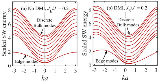
Figure 3. Dispersion relations for the discrete spin-wave (SW) modes in a ferromagnetic nanostripe with width parameter $N=12$ for the case where the exchange interactions dominate over the dipole–dipole interaction effects. The SW energies in units of $SJ$ are shown with and without Dzyaloshinskii–Moriya interactions (DMI) by taking (a) $\alpha =0$ and (b) $\alpha =0.3$. We now assume edge exchange perturbations such that $J_E/J=0.2$, showing the existence of localized acoustic edge SW modes below the bulk band.

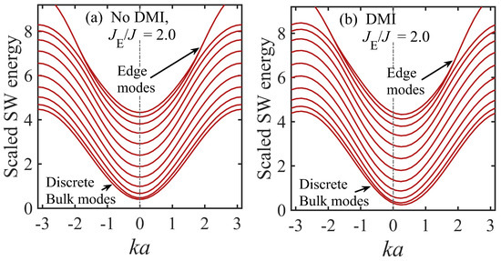
Figure 4. Dispersion relations for the discrete spin-wave (SW) modes in a ferromagnetic nanostripe with width parameter $N=12$ for the case where the exchange interactions dominate over the dipole–dipole interaction effects. The SW energies in units of $SJ$ are shown with and without Dzyaloshinskii–Moriya interactions (DMI) by taking (a) $\alpha =0$ and (b) $\alpha =0.3$. We now assume edge exchange perturbations such that $J_E/J=2.0$, showing the existence of localized optic edge modes above the bulk band.

The dispersion plots in Figure 4a,b illustrate the effects of having a $J_E/J$ ratio sufficiently above unity. For the purpose of illustration we take here $J_E/J=$ 2.0 and it is seen that again there are two modes (almost degenerate) split off from the bulk region, but in this case they occur at larger energies and for larger magnitude of the wave vector (roughly $\left|ka\right|>\pi /2$ in this example). They can be referred to as optic-type SW modes. We shall see from the SW amplitude results presented later in this section that the spatial variations of the acoustic and optic edge modes across the nanostripe widths are quite different.

3.2. General Dipole-Exchange Case

We now present results for the general case where the dynamic effects of the dipole–dipole interactions are included for the SWs, as well the bilinear (symmetric) exchange and the DMI (antisymmetric) exchange. A dimensionless parameter $d={\left(g\mu \right)}^2/J{a}^3$ may be introduced as a measure of the dipole–dipole interaction strength relative to the bilinear exchange interaction J. Values for d in real magnetic materials typically lie in the approximate range 0.002 to 0.02, although they can be much larger in some cases, e.g., $d\sim 0.5$ in GdCl₃ [59]. In Figure 5 we show the dipole-exchange SW dispersion curves for a nanostripe. There are two main differences compared with the previous section. First, we have shown examples with a larger stripe width (corresponding to $N=24$), meaning 24 SW branches. Second, the dipole–dipole interactions are taken into account with $d=0.02$ and we assume $\alpha =0.3$ for DMI, as before. Here, we have taken $J_E/J=1.0$, so a comparison can be made between Figure 2b and Figure 5a with and without dipole–dipole interactions, respectively. We comment first that the increased value for N has led to the SW band remaining essentially the same in its energy range while the separation between modes is correspondingly reduced. Overall, the two figures mentioned above are similar to one another, but a closer inspection shows that the dipole–dipole interactions have a significant effect, e.g., they give rise to SW energy shifts at small wave vectors. This property is illustrated more explicitly in Figure 5b, where the rectangular region in Figure 5a is enlarged and compared with the dispersion results in the absence of the dipolar effects (also when $N=24$).

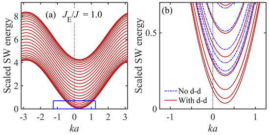
Figure 5. Dispersion relations for the discrete spin-wave (SW) modes in a ferromagnetic nanostripe with increased width parameter $N=24$ when dipole–dipole (d-d) interactions effects are included with $d=0.02$ and $J_E/J=1.0$. We have assumed $\alpha =0.3$. Panel (a) shows the behaviour over the full range of $ka$. The small- wave–vector region corresponding to the blue rectangle is shown enlarged in panel (b), where a comparison is included with the SW results in the absence of dipole–dipole interactions (blue dashed curves).

We comment that both the static (at $k=0$) and dynamic (occurring at nonzero k) effects of the dipole–dipole interactions are taken into account. As specified earlier, the equilibrium spin orientations correspond to the out-of-plane direction along the z axis. This requires that the applied field $B_0$ must exceed the static demagnetizing field $B_{demag}$, which is due to the dipole–dipole interactions, otherwise an SW instability would occur. For the example given here we estimate that $g{\mu }_B{B}_{demag}/SJ\simeq 0.19$; so, $B_0\simeq 2.1B_{demag}$.

Another similar comparison is made in Figure 6, taking now $J_E/J=0.2$ for which we previously predicted an acoustic edge SW mode (see Figure 3 for the exchange-dominated case). The inclusion of dipole–dipole interactions does not change this qualitative behaviour overall, as may be seen from Figure 6a. The enlarged area shown in Figure 6b, along with corresponding calculations for the exchange-dominated limit, emphasizes the significant differences when the dipolar effects are included.

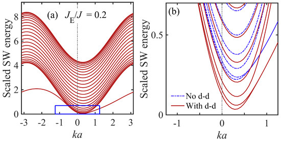
Figure 6. Dispersion relations for the discrete spin-wave (SW) modes in a ferromagnetic nanostripe with increased width parameter $N=24$ when dipole–dipole (d-d) interactions effects are included with $d=0.02$ and $J_E/J=0.2$. We have assumed $\alpha =0.3$. Panel (a) shows the behaviour over the full range of $ka$. The small- wave-vector region corresponding to the blue rectangle is shown enlarged in panel (b), where a comparison is included with the SW results in the absence of dipole–dipole interactions (blue dashed curves).

Finally, in Figure 7 we present some results for the variation in the SW spatial amplitudes across the width of the nanostripe (as represented by the row number n introduced in Section 2.1). Specifically, we plot the SW amplitudes, which are calculated from the eigenvectors of the dynamical matrix, as explained in Section 2.2. Three cases are shown, which are all for the dipole-exchange regime with $d=0.02$ and $N=24$ as in Figure 5 and Figure 6; they correspond to (a) a bulk SW mode when $J_E/J=1.0$, (b) an acoustic edge SW mode when $J_E/J=0.2$, and (c) an optic edge SW mode when $J_E/J=2.0$. The wave vector and energy values for each case are provided in the caption to Figure 7. As anticipated, Figure 7a shows a standing-wave profile across the width, while Figure 7b shows a mode localized at each edge and with an exponential-like decay away from the edge. Figure 7c also displays localization for the optic edge mode but there is an alternation in sign (meaning a 180° phase change) in going from one row to the next.

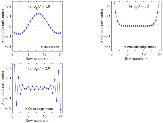
Figure 7. The spin-wave (SW) amplitudes plotted versus row number n for a nanostripe with $N=24$ in the dipole-exchange case: (a) one of the lowest bulk modes when $J_E/J=1.0$ where the scaled energy (in units of $SJ$) is equal to 1.50 and $ka=1.57$; (b) an acoustic edge mode with scaled energy 0.64 and $ka=1.57$; and (c) an optic edge mode with scaled energy 6.18 and $ka=1.76$.

4. Discussion

In conclusion, we have presented calculations for the dipole-exchange SW modes in ferromagnetic nanostripes (or nanoribbons) in the presence of interfacial DMI. We point out that the static magnetic field $B_0$ and sample magnetization are taken to be along the z direction perpendicular to the plane of the nanostripe. Most of the previous studies for DMI in planar structures (films, stripes and lateral arrays of stripes) have been for the magnetization along the easy direction in the plane, but see References [30,60] for examples of DMI studies in films when the magnetization is in the perpendicular orientation. Our focus is on finite-width effects in stripe geometries when localized edge SW modes may occur. Our chosen configuration requires that $B_0$ must be sufficiently large that it exceeds the static demagnetizing field that originates from the dipole–dipole interactions. Alternatively, the perpendicular orientation may be stabilized by an out-of-plane single-ion anisotropy as in Co/Pt ultrathin bilayers [30].

We found that the effects of DMI on the SWs include (i) a shift of the SW minimum energy away from $k=0$ by an amount that depends on the magnitude and sign of the DMI and (ii) a characteristic nonreciprocity in the SW propagation along the longitudinal (or y) direction. Our calculations allowed for the possibility that the dominant exchange parameter at the lateral edges of the nanostripe might be different from its value in the bulk of the material (due to perturbed electronic wave functions near an edge). A consequence of this property was the prediction of localized edge SWs, which could either be of the acoustic or optic type (coming below or above the bulk band). It was shown that the edge modes, which have amplitudes that decay with distance from the edges, also have very pronounced nonreciprocal characteristics with respect to their k dependence. Numerical examples were included to illustrate the spatial dependence of the bulk-like (or standing) SWs and the localized edge SWs. The calculated mode energies and shifts were found to depend sensitively on the stripe width (through parameter N) and on the ratio $J_E/J$ of exchange parameters.

The theoretical methods developed here are suitable for applications to ferromagnetic metals such as Fe or permalloy that can exhibit DMI when interfaced with an appropriate heavy metal substrate. Computations for nanostripe widths ($W=Na$) with N as large as 100 or more and a typical value of $a\sim 5$ nm for many metals are feasible, meaning W can be of the order 0.5 μm or more. With relatively minor adaptations, applications can be made to stripes formed from antiferromagnetic materials, such as Mn interfaced with Pt [61], or ferrimagnetic materials, such as Tb₃Fe₅O₁₂ (terbium iron garnet) interfaced with a heavy metal [62], using a two-sublattice model for the spin Hamiltonian. Other extensions of this work could be to stripes that are thicker in the vertical (or z) direction and/or to arrays of stripes arranged laterally as in a magnonic crystal.

Finally, we mention that it would be of interest to study nanostripes in which the DMI axial vector, as introduced in Equation (1), can lie along other crystallographic directions and/or different directions relative to the interface. Here, we took this vector to be z directed and along the magnetization direction. However, some recent studies have illustrated the capability to control or manipulate the DMI, e.g., by introducing an oxide [63] or ferroelectric [64] material at the interface, by varying the magnetic layer thickness [29], or by employing a film geometry with perpendicular magnetization [60]. Thus, other choices for the DMI axial vector in our stripe geometry can be made, and our preliminary considerations show that they may lead to novel results with spin canting and modified SW properties (e.g., see analogous recent studies for DMI directional effects in nanoring geometries [54]).

References

- Dzyaloshinskii, I.Y. Thermodynamic theory of weak ferromagnetism in antiferromagnetic substances. Sov. Phys. JETP 1957, 5, 1259. [Google Scholar]
- Dzyaloshinsky, I. A Thermodynamic theory of weak ferromagnetism of antiferromagnetics. J. Phys. Chem. Solids 1958, 4, 241. [Google Scholar] [CrossRef]
- Moriya, T. Anisotropic superexchange interaction and weak ferromagnetism. Phys. Rev. 1960, 120, 91. [Google Scholar] [CrossRef]
- Turov, E.A.; Guseinov, N.G. Magnetic resonance in rhombohedral weak ferromagnetics. Sov. Phys. JETP 1960, 11, 955. [Google Scholar]
- Melcher, R.L. Linear contribution to spatial dispersion in the spin-wave spectrum of ferromagnets. Phys. Rev. Lett. 1973, 30, 125. [Google Scholar] [CrossRef]
- Zakeri, K.; Zhang, Y.; Prokop, J.; Chuang, T.; Sakr, N.; Tang, W.X.; Kirschner, J. Asymmetric spin-wave dispersion on Fe(110): Direct evidence of the Dzyaloshinskii-Moriya interaction. Phys. Rev. Lett. 2010, 104, 137203. [Google Scholar] [CrossRef]
- Moon, J.H.; Seo, S.M.; Lee, K.J.; Kim, K.W.; Ryu, J.; Lee, H.W.; McMichael, R.D.; Stiles, M.D. Spin-wave propagation in the presence of interfacial Dzyaloshinskii-Moriya interaction. Phys. Rev. B 2013, 88, 184404. [Google Scholar] [CrossRef]
- Cortés-Ortuno, D.; Landeros, P. Influence of the Dzyaloshinskii-Moriya interaction on the spin-wave spectra of thin films. J. Phys. Condens. Matter 2013, 25, 156001. [Google Scholar] [CrossRef] [PubMed]
- Di, K.; Zhang, V.L.; Lim, H.S.; Ng, S.C.; Kuok, M.H.; Yu, J.; Yoon, J.; Qiu, X.; Yang, H. Direct observation of the Dzyaloshinskii-Moriya interaction in a Pt/Co/Ni film. Phys. Rev. Lett. 2015, 114, 047201. [Google Scholar] [CrossRef] [PubMed]
- Gallardo, R.A.; Corteś-Ortuno, D.; Troncoso, R.E.; Landeros, P. Spin waves in thin films and magnonic crystals with Dzyaloshinskii-Moriya interactions. In Three-Dimensional Magnonics; Gubbiotti, G., Ed.; Jenny Stanford: Singapore, 2019; p. 121. [Google Scholar]
- Camley, R.; Livesey, K.L. Consequences of the Dzyaloshinskii-Moriya interaction. Surf. Sci. Rep. 2023, 78, 100605. [Google Scholar] [CrossRef]
- Kuanr, B.K.; Veerakumar, V.; Mishra, S.R.; Camley, R.E.; Celinski, Z. Nonreciprocal microwave devices based on magnetic nanowires. Appl. Phys. Lett. 2009, 94, 202505. [Google Scholar] [CrossRef]
- Barman, A.; Gubbiotti, G.; Ladak, S.; Adeyeye, A.O.; Krawczyk, M. The 2021 Magnonics Roadmap. J. Phys. Condens. Mater 2021, 33, 413001. [Google Scholar] [CrossRef] [PubMed]
- Tomasello, R.; Martinez, E.; Zivieri, R.; Torres, L.; Carpentieri, M.; Finocchio, G. A strategy for the design of skyrmion racetrack memories. Nat. Sci. Rep. 2014, 4, 6784. [Google Scholar] [CrossRef]
- Chen, J.; Yu, H.; Gubbiotti, G. Unidirectional spin-wave propagation and devices. J. Phys. D Appl. Phys. 2022, 55, 123001. [Google Scholar] [CrossRef]
- Luo, S.; Song, M.; Li, X.; Zhang, Y.; Hong, J.; Yang, X.; Zou, X.; Xu, N.; You, L. Reconfigurable skyrmion logic gates. Nano Lett. 2018, 18, 1180–1184. [Google Scholar] [CrossRef]
- Shen, L.; Zho, Y.; Shen, K. Programmable skyrmion-based logic gates in a single nanotrack. Phys. Rev. B 2023, 107, 054437. [Google Scholar] [CrossRef]
- Tretiakov, O.A.; Abanov, A. Current driven magnetization dynamics in ferromagnetic nanowires with a Dzyaloshinskii-Moriya interaction. Phys. Rev. Lett. 2010, 105, 157201. [Google Scholar] [CrossRef]
- Freimuth, F.; Blugel, S.; Mokrousov, Y. Relation of the Dzyaloshinskii-Moriya interaction to spin currents and to the spin-orbit field. Phys. Rev. B 2017, 96, 054403. [Google Scholar] [CrossRef]
- Chumak, A.V.; Schultheiss, H. Magnonics: Spin waves connecting charges, spins and photons. J. Phys. D Appl. Phys. 2017, 50, 300201. [Google Scholar] [CrossRef]
- Sharma, M.; Kumar, R.; Chauhan, A.; Kuanr, B.K. Magnetization dynamics of ferromagnetic nanostructures for spintronics and bio-medical applications. In Multifunctional Materials; Tripathy, D.B., Gupta, A., Jain, A.K., Eds.; Scrivener Publishing: Beverly, MA, USA, 2025. [Google Scholar] [CrossRef]
- Haze, M.; Yoshida, Y.; Hasegawa, Y. Experimental verification of the rotational sense and type of chiral spin spiral structure by spin-polarized scanning tunneling microscopy. Sci. Rep. 2016, 7, 13269. [Google Scholar] [CrossRef]
- Hrabec, A.; Luo, Z.; Heyderman, L.J.; Gambardella, P. Synthetic chiral magnets promoted by the Dzyaloshinskii–Moriya interaction. Appl. Phys. Lett. 2020, 117, 130503. [Google Scholar] [CrossRef]
- Gallardo, R.; Alvarado-Seguel, P.; Landeros, P. Unidirectional chiral magnonics in cylindrical synthetic antiferromagnets. Phys. Rev. Appl. 2022, 18, 054044. [Google Scholar] [CrossRef]
- Heide, M.; Bihlmayer, G.; Blügel, S. Dzyaloshinskii-Moriya interaction accounting for the orientation of magnetic domains in ultrathin films: Fe/W(110). Phys. Rev. B 2008, 78, 140403. [Google Scholar] [CrossRef]
- DeJong, M.D.; Livesey, K.L. Domain walls in finite-width nanowires with interfacial Dzyaloshinskii-Moriya interaction. Phys. Rev. B 2017, 95, 054424. [Google Scholar] [CrossRef]
- Muratov, C.; Slastikov, V.V.; Kolesnikov, A.G.; Tretiakov, O.A. Theory of the Dzyaloshinskii domain-wall tilt in ferromagnetic nanostrips. Phys. Rev. B 2017, 96, 134417. [Google Scholar] [CrossRef]
- Zakeri, K.; Zhang, Y.; Chuang, T.H.; Kirschner, J. Magnon lifetimes on the Fe(110) surface: The role of spin-orbit coupling. Phys. Rev. Lett. 2012, 108, 197205. [Google Scholar] [CrossRef] [PubMed]
- Cho, J.; Kim, N.H.; Lee, S.; Kim, J.S.; Lavrijsen, R.; Solignac, A.; Yin, Y.; Han, D.S.; van Hoof, N.J.J.; Swagten, H.J.M.; et al. Thickness dependence of the interfacial Dzyaloshinskii–Moriya interaction in inversion symmetry broken systems. Nat. Commun. 2015, 6, 7635. [Google Scholar] [CrossRef]
- Belmeguenai, M.; Adam, J.P.; Roussigné, Y.; Eimer, S.; Devolder, T.; Kim, J.V.; Cherif, S.M.; Stashkevich, A.; Thiaville, A. Interfacial Dzyaloshinskii-Moriya interaction in perpendicularly magnetized Pt/Co/AlOx ultrathin films measured by Brillouin light spectroscopy. Phys. Rev. B 2015, 91, 180405. [Google Scholar] [CrossRef]
- Stashkevich, A.A.; Belmeguenai, M.; Roussigné, Y.; Cherif, S.M.; Kostylev, M.; Gabor, M.; Lacour, D.; Tiusan, C.; Hehn, M. Experimental study of spin-wave dispersion in Py/Pt film structures in the presence of an interface Dzyaloshinskii-Moriya interaction. Phys. Rev. B 2015, 91, 214409. [Google Scholar] [CrossRef]
- Chaurasiya, A.K.; Banerjee, C.; Pan, S.; Sahoo, S.; Choudhury, S.; Sinha, J.; Barman, A. Direct observation of interfacial Dzyaloshinskii-Moriya interaction from asymmetric spin-wave propagation in W/CoFeB/SiO2 heterostructures down to sub-nanometer CoFeB thickness. Sci. Rep. 2016, 6, 32592. [Google Scholar] [CrossRef]
- Tacchi, S.; Troncoso, R.E.; Ahlberg, M.; Gubbiotti, G.; Madami, M.; Akerman, J.; Landeros, P. Interfacial Dzyaloshinskii-Moriya interaction in Pt/CoFeB films: Effect of the heavy-metal thickness. Phys. Rev. Lett. 2017, 118, 147201. [Google Scholar] [CrossRef] [PubMed]
- Gallardo, R.A.; Alvarado-Seguel, P.; Brevis, F.; Gonzalez-Fuentes, C.; Roldan-Molina, A.; Lenz, K.; Lindner, J.; Landeros, P. Spin-wave non-reciprocity in magnetization-graded ferromagnetic films. New J. Phys. 2019, 21, 033026. [Google Scholar] [CrossRef]
- Kostylev, M. Interface boundary conditions for dynamic magnetization and spin wave dynamics in a ferromagnetic layer with the interface Dzyaloshinskii-Moriya interaction. J. Appl. Phys. 2014, 115, 233902. [Google Scholar] [CrossRef]
- Mruczkiewicz, M.; Krawczyk, M. Influence of the Dzyaloshinskii-Moriya interaction on the FMR spectrum of magnonic crystals and confined structures. Phys. Rev. B 2016, 94, 024434. [Google Scholar] [CrossRef]
- Bouloussa, H.; Roussigné, Y.; Belmeguenai, M.; Stashkevich, A.; Chérif, S.M.; Pollard, S.D.; Yang, H. Dzyaloshinskii-Moriya interaction induced asymmetry in dispersion of magnonic Bloch modes. Phys. Rev. B 2020, 102, 014412. [Google Scholar] [CrossRef]
- Silvani, R.; Alumni, M.; Tacchi, S.; Carlotti, G. Effect of the interfacial Dzyaloshinskii–Moriya interaction on the spin wave eigenmodes of isolated stripes and dots magnetized in-plane: A micromagnetic study. Appl. Sci. 2021, 11, 2929. [Google Scholar] [CrossRef]
- Gallardo, R.; Alvarado-Seguel, P.; Landeros, P. Spin-wave channeling in magnetization-graded nanostrips. Nanomaterials 2022, 12, 2785. [Google Scholar] [CrossRef] [PubMed]
- Gallardo, R.A.; Alvarado-Seguel, P.; Brevis, F.; Gonzalez-Fuentes, C.; Gonzalez, J.W.; Lenz, K.; Lindner, J.; Roldan-Molina, A. Nonreciprocal spin wave channeling in ferromagnetic/heavy-metal nanostrips. Results Phys. 2024, 67, 108057. [Google Scholar] [CrossRef]
- Nguyen, H.T.; Nguyen, T.M.; Cottam, M.G. Dipole-exchange spin waves in ferromagnetic stripes with inhomogeneous magnetization. Phys. Rev. B 2007, 76, 134413. [Google Scholar] [CrossRef]
- Lupo, P.; Haghshenasfard, Z.; Cottam, M.G.; Adeyeye, A.O. Ferromagnetic resonance study of interface coupling for spin waves in narrow NiFe/Ru/NiFe multilayer nanowires. Phys. Rev. B 2016, 94, 214431. [Google Scholar] [CrossRef]
- Gubbiotti, G.; Tacchi, S.; Nguyen, H.T.; Madami, M.; Carlotti, G.; Nakono, K.; Ono, T.; Cottam, M.G. Coupled spin waves in trilayer films and nanostripes of permalloy separated by nonmagnetic spacers: Brillouin light scattering and theory. Phys. Rev. B 2013, 87, 094406. [Google Scholar] [CrossRef]
- Gubbiotti, G.; Zhou, X.; Haghshenasfard, Z.; Cottam, M.G.; Adeyeye, A.O.; Kostylev, M. Interplay between intra- and inter-nanowires dynamic dipolar interactions in the spin wave band structure of Py/Cu/Py nanowires. Nat. Sci. Rep. 2019, 9, 4617. [Google Scholar] [CrossRef] [PubMed]
- Cottam, M.G.; Haghshenasfard, Z.; Adeyeye, A.O.; Gubbiotti, G. Dipole-exchange theory of magnons in structured composite nanowires and magnonic crystal arrays. In Three-Dimensional Magnonics; Gubbiotti, G., Ed.; Jenny Stanford Publishing: Singapore, 2019; p. 1. [Google Scholar]
- Aharoni, A. Introduction to the Theory of Ferromagnetism; Clarendon Press: Oxford, UK, 1996. [Google Scholar]
- Gurevich, A.G.; Melkov, G.A. Magnetization Oscillations and Waves; CRC Press: Boca Raton, FL, USA, 1996. [Google Scholar] [CrossRef]
- Stancil, D.D.; Prabhakar, A. Spin Waves: Theory and Applications; Springer: Berlin/Heidelberg, Germany, 2009. [Google Scholar]
- Gubbiotti, G. (Ed.) Three-Dimensional Magnonics; Jenny Stanford Publishing: Singapore, 2019. [Google Scholar]
- Kronmüller, H. General Micromagnetic Theory and Applications; Wiley: New York, NY, USA, 2019. [Google Scholar]
- Coey, J.M.D. Magnetism and Magnetic Materials; Cambridge University Press: Cambridge, UK, 2010. [Google Scholar]
- White, R.M. Quantum Theory of Magnetism: Magnetic Properties of Materials, 3rd ed.; Springer: Berlin/Heidelberg, Germany, 2007. [Google Scholar]
- Hussain, B.; Cottam, M.G. Dipole-exchange spin waves in unsaturated ferromagnetic nanorings with interfacial Dzyaloshinski-Moriya interactions. J. Appl. Phys. 2022, 132, 193901. [Google Scholar] [CrossRef]
- Hussain, B.; Cottam, M.G. Spin waves in ferromagnetic nanorings with interfacial Dzyaloshinskii-Moriya interactions: II. Directional effects. Nanomaterials 2024, 14, 286. [Google Scholar] [CrossRef]
- Holstein, T.; Primakoff, H. Field dependence of the intrinsic domain magnetization of a ferromagnet. Phys. Rev. 1940, 58, 1098. [Google Scholar] [CrossRef]
- Rezende, S.M. Fundamentals of Magnonics; Springer: Berlin/Heidelberg, Germany, 2020. [Google Scholar]
- Wolfram, T.; Dewames, R.E. Surface dynamics of magnetic materials. Prog. Surf. Sci. 1972, 2, 233. [Google Scholar] [CrossRef]
- Nguyen, T.M.; Cottam, M.G. Microscopic theory of dipole-exchange spin wave excitations in ferromagnetic nanowires. Phys. Rev. B 2005, 71, 094406. [Google Scholar] [CrossRef]
- Clover, R.B.; Wolf, W.P. High frequency specific heat measurements and exchange constants of GdCl3. Solid State Commun. 1968, 5, 331. [Google Scholar] [CrossRef]
- Hrabec, A.; Porter, N.A.; Wells, A.; Benitez, M.J.; Burnell, G.; McVitie, S.; McGrouther, D.; Moore, T.A.; Marrows, C.H. Measuring and tailoring the Dzyaloshinskii-Moriya interaction in perpendicularly magnetized thin films. Phys. Rev. B 2014, 90, 020402(R). [Google Scholar] [CrossRef]
- Akanda, M.R.K.; Park, J.; Lake, R.K. Interfacial Dzyaloshinskii-Moriya interaction of antiferromagnetic materials. Phys. Rev. B 2020, 102, 224414. [Google Scholar] [CrossRef]
- Fedel, S.; Villa, M.; Damerio, S.; Demiroglu, E.; Deger, C.; Gazquez, J.; Avci, C.O. Evidence of long-range Dzyaloshinskii-Moriya interaction at ferrimagnetic insulator/nonmagnetic metal interfaces. Adv. Funct. Mater. 2025, 35, 2418653. [Google Scholar] [CrossRef]
- Arora, M.; Shaw, J.M.; Nembach, H.T. Variation of sign and magnitude of the Dzyaloshinskii-Moriya interaction of a ferromagnet with an oxide interface. Phys. Rev. B 2020, 101, 054421. [Google Scholar] [CrossRef]
- Zhang, B.H.; Hou, Y.S.; Wang, Z.; Wu, R.Q. Tuning Dzyaloshinskii-Moriya interactions in magnetic bilayers with a ferroelectric substrate. Phys Rev. B 2021, 103, 0514417. [Google Scholar] [CrossRef]
Disclaimer/Publisher’s Note: The statements, opinions and data contained in all publications are solely those of the individual author(s) and contributor(s) and not of MDPI and/or the editor(s). MDPI and/or the editor(s) disclaim responsibility for any injury to people or property resulting from any ideas, methods, instructions or products referred to in the content. |
© 2025 by the authors. Licensee MDPI, Basel, Switzerland. This article is an open access article distributed under the terms and conditions of the Creative Commons Attribution (CC BY) license (https://creativecommons.org/licenses/by/4.0/).