Genetic Algorithms for Piston and Tilt Detection by Using Young Patterns

Abstract

We present some numerical results on piston and tilt detection by using the Young experiment with Genetic Algorithms (GAs). We have simulated the cophasing of a flat surface by following the experimental setup and the mathematical model for Optical Path Difference (OPD) in the Young experiment to characterize piston and tip–tilt misalignment images in the order of a few nanometers, considering diffraction effects and random noise of 5%. Thus, the best fitness obtained by the genetic algorithm is considered as a determining factor to decide a complete error measurement because the proposed algorithm is capable of extracting the values of piston and tilt separately, regardless of which error is present or both. As a result, we have developed a study on piston detection from (0.001, 10) mm with a tilt present in the same pattern from (0, $\lambda /2$) by using GAs embedded in a computational application.

1. Introduction

During the stage of segmented surface alignment, one problem to solve is how to minimize the relative piston error between adjacent segments. This process is known as cophasing. Once each relative piston value on the segmented surface has been minimized, the root mean square (RMS) piston error must be considered.

Cophasing is one of the specific tasks associated with segmented telescopes, and it requires the development of active control over three degrees of freedom for each individual segment: translation along the optical axis (piston), and rotation about two perpendicular axes (tip–tilt). A piston error is typically on the order of a wavelength or a fraction thereof; physically, it manifests as a step between adjacent segments. Therefore, to achieve proper alignment, the misaligned segment must be repositioned such that the relative piston error falls within a fraction of the wavelength, typically better than $\lambda /40$ RMS for the entire segmented surface [1].

Segmented surface cophasing has become an essential topic for the scientific community engaged in the construction of large optical telescope surfaces. This is because the building of segmented mirrors is one of the few feasible ways to reduce manufacturing and transportation costs for large-aperture systems. Several issues arise when aligning such telescopes. For instance, once the telescope is assembled, all optical and electronic components of the active system must be tested because the orientation of each segment affects image quality in the observation plane.

The main techniques used for cophasing in the Keck telescopes in Hawaii (USA) include the algorithms of Chanan et al. [1]. More recently, the GRAVITY instrument at VLTI has implemented advanced fringe-tracking and piston reconstruction techniques to improve long-baseline interferometry, even under atmospheric turbulence [2].

For segmented mirror telescopes like the ELT, maintaining phase continuity across segments is critical. Wang et al. proposed a method for detecting piston errors under turbulence using optical techniques that remain accurate even in degraded vision conditions [3].

Rousseaux et al. presented a low-light piston and tilt sensor combining a diffraction grating and a micro-lens array for the simultaneous measurement of phase and inclination [4]. He et al. introduced a vortex-based interferometric method that encodes piston information in spiral-shaped fringe patterns [5].

To address large initial piston errors, Qin et al. proposed a dynamic adjustment multiwavelength interference method, capable of correcting piston mismatches greater than 1 mm with nanometric precision [6].

Li and Wang introduced a frequency-domain filtering method combined with convolutional neural networks to estimate piston values from focal-plane intensity distributions [7]. Similarly, Guerra-Ramos et al. employed deep learning with CNN-RNN architectures to retrieve global piston values from segmented diffraction patterns [8].

The present work contributes to this evolving landscape by proposing a GA-based algorithm for the piston and tilt detection from synthetic Young interferometric patterns. The proposed method is resilient to tilt-induced distortions and does not require preprocessing to isolate piston effects. Currently, the computational optimization algorithm is being successfully applied in the context of the cophasing topic as in the case of [9], where a hybrid algorithm based on phase diversity aimed at massive sub-apertures of the segmented primary mirror is presented. The authors propose a genetic algorithm to obtain initial values of Zernike aberration coefficients. After initial alignment values for the segmented primary mirror analog system, linearization of these values is processed. Furthermore, in [10] a separately-polished segmented mirrors to cophasing surface shape error, optimizing a segmented mirror with a global radius of curvature was proposed, as well as a multi-fidelity surrogates based on sensitivity accuracy and a multi-island genetic algorithm was applied in order to optimized a segmented mirror. Other work where optimization algorithm are used is in [11], where a simulations and hardware realization of a simulated annealing algorithm in an active optical system, with sparse segments, generating a local optimization of piston and tip–tilt errors have been proposed. In most of the works developed for cophasing of a segmented surface, the performance dynamic range is always involved, as in the case of [12], where a fine alignment of the great James Webb Space Telescope with a genetic algorithm has been optimized in the last alignment stage for fine-phasing. Here, the optical elements were handled with seven degrees of freedom. In addition, three parameters or genes were handled in the proposed genetic algorithm. Inside the optimization process, the neural net is also being used for minimizing the phase errors, such as the work of [13], here a convolutional neural network is proposed to distinguish the piston error range of each sub-mirror, given on the phase cophasing phase of the segmented optical mirrors, since the Shack-Hartmann wavefront sensor is not sensitive to the sub-mirror piston error. This method surpasses the limits of the detection range when different wavelengths are used. In addition, a simulation experiment was introduced.

This paper is organized as follows. Section 2 introduces the theoretical framework. Section 3 explains the use of a constant term in the Young experiment to characterize piston and tilt. Section 4 describes how GA is applied for parameter extraction. Section 5 presents the experimental setup, and Section 6 discusses the results and conclusions.

2. Theoretical Basis

Three theoretical foundations were taken into consideration to support the present work.

The first is a classical study on the phase alignment of segmented mirrors using a digital Zygo interferometer by Jian Bai et al. [14]. In that work, it is established that the piston term is associated with an axial displacement along the optical axis of the segmented surface under test. This axial displacement is implicitly present in the defocusing component of the wavefront aberration.

The second foundation relates to a previous study on piston detection by Salinas-Luna et al. [15], where cophasing was achieved by analyzing the defocusing term. In that work, it was shown that defocusing can be interpreted as a piston when the phase shift is on the order of the wavelength and remains constant across the surface. Otherwise, it is considered classical defocus, which is nonlinear in nature [16]. Another interesting insight comes from experimental piston detection using the Ronchi test [17], where it was demonstrated that a small focus shift for each segment could be detected if the classical Ronchi ruling was laterally displaced.

Building on that idea, we have simulated piston by adding a constant term to the optical path difference (OPD) in Young’s experiment. The effect of the piston manifests as a change in fringe width for the displaced segment, modeled by displacing both secondary sources. In contrast, tilt or tip was simulated by displacing only one secondary source, producing a shift in the zero-order fringe of the irradiance. The resulting fringe patterns for both cases are analyzed in the following sections.

Furthermore, in a previous geometrical analysis [17], the piston term was related to the transverse aberration in the Ronchi test using ray tracing, neglecting diffraction effects by employing high-frequency Ronchi rulings. Even though diffraction was ignored, the operation range of the system could be characterized.

Finally, according to Hopkins’ theory of wave aberrations [18], adding a constant to the wavefront results in a defocusing effect. Conversely, a defocus aberration in the wavefront can be interpreted as the addition of a constant phase term.

3. Piston and Tip-Tilt in the Young’s Experiment

Initially, the conceptual design of this work was thought of as a prototype of a segmented surface with a pair of flat mirror segments. This is because the mathematical model of Young’s experiment is more adaptable for this type of surfaces, since secondary sources could be placed on any part of the mirror surface, and thus it would be possible to detect easier tip tilts in other directions. In the piston case, the secondary sources can be placed at any point on the optical surface. Consequently, we intend to perform the experiment with geometrical tests in order to make a comparison.

To begin our numerical analysis, we have considered movements of the position of the secondary sources to characterize errors in a segmented surface and it allows the using of the Young experiment.

Following Figure 1, a segmented surface with piston error can be characterized in our work by using a theoretical analysis for the OPD in the experiment of Young [19], Figure 1. Well known, that the interference fringes are produced by the light recombination of the secondary sources $S_1,S_2$ (separated by a distance d) on an observation plane $(x,y)$ (the distance from the sources plane and observation plane is a).

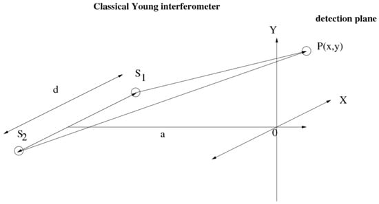
Figure 1. Reference system for the point secondary sources.

So that, the irradiance behavior in two adjacent Young’s experiments is depicted in Figure 2, when two masks with circular apertures (secondary sources) are used to co-phase a flat segmented surface. Here, classical Young’s experiment is taken for reference mirror and another for the displaced mirror (pistoned Young’s experiment). It is worth mentioning that in each Young experiment the complete phase is known; however, half of each one is eliminated to make a comparison between each case.

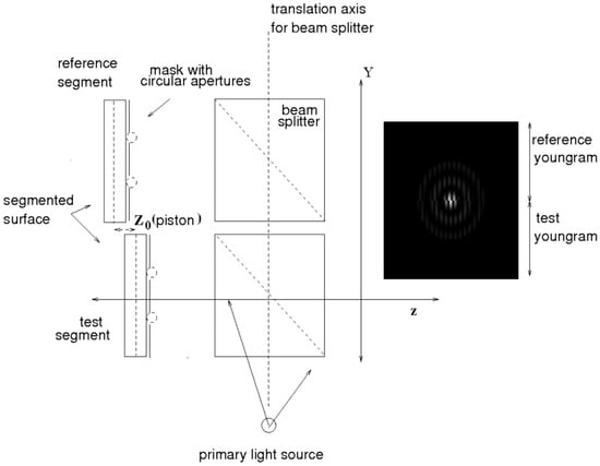
Figure 2. Diagram to characterize piston with the Young interferometer. Right image obtained in the Y-axis detection plane is for comparing (up) Classical Young’s experiment with (down) Pistoned Young’s experiment; a youngram is an interferogram generated by Young’s experiment.

It is known that irradiance for the classical experiment of Young can be characterized of its physical parameters in the plane observation,

$$irradiance=4I_0{cos}^2\left(\delta \right),$$

(1)

where

$$\delta =n\kappa \left({\displaystyle \frac{xd}{a}}\right),$$

(2)

with $\kappa$ as the wave number with ($\kappa ={\displaystyle \frac{2\pi }{{\lambda }_0}}$), n is the refraction index, ($n=1$), ${\lambda }_0$ is the used wavelength and $I_0$ is the maximum value of intensity in the Young pattern. Equation (2) arises after considering two point sources and without diffraction effects.

If the Young experiment considers circular apertures with certain diameter as secondary sources, then the complete irradiance should contain two factors; the first one is a diffraction pattern as amplitude function, it depends on the shape of the geometry of the apertures, in this case is the diffraction pattern for a circular aperture. Mathematically,

$$diffraction=2J_1(\kappa ,R,q),$$

(3)

where $J_1$ is a Bessel function of order 1, R is the distance from plane of the circular apertures to observation plane, d is the aperture diameters and q is the radii of the Airys disc, it depends on

$$q=1.22\left({\displaystyle \frac{R{\lambda }_0}{2d}}\right)$$

(4)

The second one is the interference factor, it is a cosinusoidal function [20], where its phase contains the OPD information. Thus, Equation (1) can be rewritten as,

$$irradiance=4I_0{\left(diffraction\right)}^2{cos}^2\left(\delta \right).$$

(5)

On the other hand, we have obtained that a piston term can be characterized by adding to sagitta a constant term $z_0$ [15], in the order of the wavelength, and it could be also introduced in Equation (2) to generate a piston error, since a discontinuity in the phase for a step (piston), produces a change in the patterns frequency. Thus, in order to characterize the simulation of cophasing of a flat segmented surface in the classical Young in this work, we compare the fringes for the classical Young experiment (fixed segment) with the fringes of the final phase for the Young experiment where a constant, $z_0$, of the order of a multiple or fraction of the wavelength is added to the parameter a (test segment). This idea belongs to displace both sources in the segment under test by generating an expected change in the frequency of the patterns. Therefore Equation (2) can be expressed as

$$\delta =n\kappa \left({\displaystyle \frac{xd}{a\pm z_0}}\right).$$

(6)

However, in order to characterize an inclination in the Young experiment, it is necessary to displace only one source a distance $\Delta a$, maintaining the other one fixed in the test segment. Thus, to introduce tip or tilt, the sources are located in a reference axis system, see Figure 3. For the fixed source we have,

$$s_1=S_{1}P=\sqrt{a^2+y^2+{\left(x-{\displaystyle \frac{d}{2}}\right)}^2},$$

(7)

to introduce an inclination, source 2 is displaced as follows,

$$s_2=S_{2}P=\sqrt{{(a+\Delta a)}^2+y^2+{\left(x+{\displaystyle \frac{d}{2}}\right)}^2},$$

(8)

if we obtain the square and reduce these two equations, after some simplifications,

$$s_2-s_1={\displaystyle \frac{\Delta a^2+2a\Delta a+2xd}{s_2+s_1}},$$

(9)

in the practice, due to the short wavelength of the light in the visible spectrum, the fringes can be observed only if $d\ll a$, so that, x and y are also small compared with the distance a [19], in other words,

$$s_2+s_1\backsim 2a,$$

(10)

then Equation (6) can be rewritten as,

$$s_2-s_1={\displaystyle \frac{\Delta a^2+2a\Delta a+2xd}{2a}},$$

(11)

where $\Delta a$ produces a change in Equation (2) for the phase, generating a tip or tilt, following mathematical expression, we have

$$\delta =\kappa \left({\displaystyle \frac{\Delta a^2+2a\Delta a}{2a}}+{\displaystyle \frac{xd}{a}}\right).$$

(12)

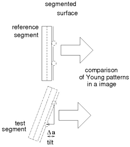
Figure 3. Diagram to generate an image with tilt in the Young interferometer in this work.

As can be observed in Equation (9), the interference term $\left({\displaystyle \frac{xd}{a}}\right)$ appears again for the case of inclinations the same way as in the typical case of Young’s experiment, Equation (2). Therefore if we want to generate a piston error, then it is compare the Young fringes in two adjacent segments, where the fringes for the classical Young experiment $\left({\displaystyle \frac{xd}{a}}\right)$ are used for the fixed segment and for the segment with piston a constant $z_0=m\lambda$ is added to variable $a\left({\displaystyle \frac{xd}{a\pm z_0}}\right)$, as it was previously mentioned.

For the case of the contributions for tip or tilt, $\Delta a$, on the phase difference $\delta$ (where $z_0=0$), it has been obtained $\left({\displaystyle \frac{\Delta a^2+2a\Delta a}{2a}}+{\displaystyle \frac{xd}{a}}\right)$, where now the interference term, $\left({\displaystyle \frac{xd}{a}}\right)$, can be considered as the initial phase in this experiment.

The equation for the irradiance in the Young experiment as function of the combined contributions for piston, $z_0$, and tip or tilt, $\Delta a$, on the phase difference, $\delta$, can be expressed as,

$$irradiance=4I_0{\left(diffraction\right)}^2{cos}^2\left[\kappa \left({\displaystyle \frac{\Delta a^2+2a\Delta a}{2a}}+{\displaystyle \frac{xd}{a\pm z_0}}\right)\right].$$

(13)

In these last equations are piston and tilt in terms of the physical parameters of the Young experiment for this work. A more detailed explanation of the mathematical development for a piston-based optical system was described by Salinas-Luna et al. in [21].

4. Piston and Tip-Tilt Extraction Using GA

GA were formally introduced in the US in the 1970s by John Holland at University of Michigan, Holland [22]. A Genetic Algorithm is an adaptive heuristic search algorithm based on the evolutionary ideas of natural selection, Darwin [23] and genetics. They are used to find approximate solutions to complex problems where traditional methods may be inefficient. The flowchart of Figure 4 illustrates the steps of a typical Genetic Algorithm. Some key concepts in genetic algorithms are the following:

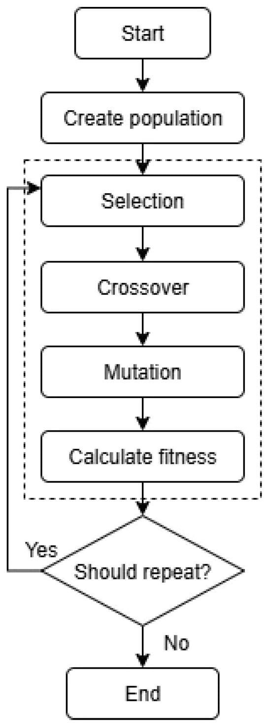
Figure 4. Flowchart of a typical Genetic Algorithm.

-

Population: A set of potential solutions, called individuals or chromosomes.

-

Fitness function: evaluates how good each solution is. Typically, the fitness value ranges from 0 to 1.0, where 1.0 denotes optimal solutions.

-

Selection: chooses the best individuals to reproduce based on fitness.

-

Crossover or recombination: combines parts of two parents to create offspring.

-

Mutation: Introduces small random changes to individuals to maintain diversity.

-

Evolution: Over successive generations, the population evolves toward better solutions, similar to how species evolve in nature through natural selection.

4.1. Solution Representation

An individual encapsulates all the parameters required to build an image. It consists of the following:

• Phenotype: a pair $⟨episton,tilt⟩\in {\Re }^2$.
• Genotype: a chain of 64 bits: an unsigned-integer value, 32 bits for piston, and 32 bits for tilt.
• Fitness: a double-precision number.
• Expected Value: a double-precision number, used for roulette selection, (see Section 4.3).

The first stage of a genetic algorithm consists of creating a random population of individuals; each individual is constructed by setting a random binary value $[0,1]$ to each bit (or gene) from its genotype. Notice that search-space exploration performed by a genetic algorithm is not aware of what exactly is being optimized; this is because genetic operators, including population creation, work exclusively with genotypes. Nevertheless, there has to be something in a genetic algorithm aware of the values we are dealing with (piston, tilt) and how are they employed in an equation intended to be minimized or maximized (Young patterns), and this is the fitness calculation, (see Section 4.2). Therefore, there has to be a way to translate a given genotype (bit sequence) into a phenotype (piston, tilt), in such a way that no two genotypes are mapped into the same phenotype, in order to avoid ambiguities. Thus, phenotype is given by the formulas:

$$piston=-10.0+((Genotype\gg 32)\wedge FFFFFFF{F}_{16})\times 20.0$$

(14)

and

$$tilt=-{\displaystyle \frac{{\lambda }_0}{1600}}+(Genotype\wedge 000000000000FFFFFFF{F}_{16})\times \left({\displaystyle \frac{{\lambda }_0}{800}}\right)/FFFFFFF{F}_{16}.$$

(15)

Notice that the 32 more significant bits of the genotype are mapped into a floating-point piston value in the range $[-10.0,10.0]$ millimeters whereas the 32 less significant bits are mapped into a floating-point tilt value in the range $\left[-{\displaystyle \frac{{\lambda }_0}{1600}},{\displaystyle \frac{{\lambda }_0}{1600}}\right]$. Some values are specified in hexadecimal format to easily indicate the largest 32-bit unsigned integer value. In tilt calculation, the effect of the ∧ (AND) operation is to keep only the 32 less significant bits of the genotype.

From the formulas above, the following holds:

$$-10.0\le piston\le 10.0,$$

(16)

in steps of $\approx 4.65\times {10}^{-9}$, and

$$-{\displaystyle \frac{{\lambda }_0}{1600}}\le tilt\le {\displaystyle \frac{{\lambda }_0}{1600}},$$

(17)

in steps of $\approx 2.91\times {10}^{-13}{\lambda }_0$.

Both ranges have to be known from start since genetic algorithms perform both exploration and exploitation inside a given enclosed search space where the best solution is expected to reside. We have decided to use the range $\left[-{\displaystyle \frac{{\lambda }_0}{1600}},{\displaystyle \frac{{\lambda }_0}{1600}}\right]$ for tilt values since it is symmetric and denotes the largest possible interval free from ambiguities, which means that no two values in this range produce exactly the same patterns. Adding a constant $i<{\displaystyle \frac{{\lambda }_0}{1600}}$ to the first value in the range, results in the same patterns as adding such a constant to the last value. As for the piston, no ambiguities were observed because the interference fringes showed a progressive widening as the piston values varied from $-45$ to 45 mm in our experiments. However, in practice, piston values range from $0.0$ to a few centimeters. Thus, we considered fair enough to use piston values in the range $(-10:10)$ to run our simulations, taking into consideration that the lower the range, the more accurate the result.

To understand better the relationship between genotype and phenotype, we analyzed the following example where a genotype is translated into a phenotype. The genotype is written in hexadecimal format to indicate that it denotes merely a sequence of bits. In order to distinguish among numbers in decimal and hexadecimal format, sub index 16 is employed for the latter case.

Assume the following chromosome was randomly generated at first, and ${\lambda }_0=0.000632$ mm, Genotype: $A71F068E94DB386C_2$.

The resulting phenotype is calculated as follows:

$$\begin{array}{cc}\hfill piston& =-10.0+((A71F068E94DB386C{2}_{16}\gg 32)/FFFFFFF{F}_{16})\times 20.0\hfill \\ \hfill & =-10.0+(A71F068E_{16}/FFFFFFF{F}_{16})\times 20.0\hfill \\ \hfill & =-10.0+(2,{803}^{\prime }828,366/4,{294}^{\prime }967,295)\times 20.0\hfill \\ \hfill & =-10.0+0.6528\times 20.0\hfill \\ \hfill & =-10.0+13.0563\hfill \\ \hfill & =3.056343\mathrm{mm}\hfill \end{array}$$

(18)

notice that the piston value falls inside our range of interest: $(-10:10)$; for tilt we have

$$\begin{array}{cc}\hfill tilt& =-{\displaystyle \frac{{\lambda }_0}{1600}}+(A71F068E94DB386C_{16}\wedge 00000000FFFFFFF{F}_{16})\times \left({\displaystyle \frac{{\lambda }_0}{800}}\right)/FFFFFFF{F}_{16}\hfill \\ \hfill & =-{\displaystyle \frac{{\lambda }_0}{1600}}+94DB386C_{16}\times \left({\displaystyle \frac{{\lambda }_0}{800}}\right)/FFFFFFF{F}_{16}\hfill \\ \hfill & =-{\displaystyle \frac{0.000632}{1600}}+2,{497}^{\prime }394,796\times \left({\displaystyle \frac{0.000632}{800}}\right)/4,{294}^{\prime }946,295\hfill \\ \hfill & =-3.95\times {10}^{-7}+4.5936\times {10}^{-7}\hfill \\ \hfill & =6.4361\times {10}^{-8}\hfill \\ \hfill & =0.000000064361\mathrm{mm}.\hfill \end{array}$$

(19)

4.2. Fitness Evaluation

In this work, every input image used in the runs of the algorithm proposed includes Gaussian noise. Some examples of input images are shown in Section 6. Hence, before running the genetic algorithm, noise is reduced by assigning every pixel the average intensity of its neighbors and itself. After this, the intensity of each of the pixels on the first row bottom-up of the top-half, i.e., row ${\displaystyle \frac{1}{2}}h$ (where h is the image height) is stored into a one-dimensional array, referred as $goal$ in the fitness algorithm, the length of which is equal to the width of the input image. In the flowchart of Figure 5, the algorithm used to remove Gaussian noise from the input image is shown.

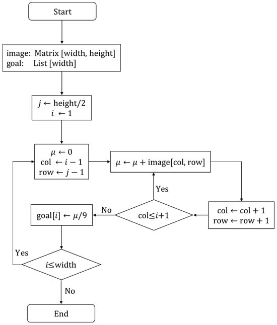
Figure 5. Algorithm 1. Removing Gaussian noise from input image.

Fitness is in terms of how far or close a given solution is from a goal image given as input. The logic of the algorithm is as follows: for every point $⟨x,\frac{h}{2}⟩$ where x in $[1,\dots w]$, we measure the irradiance by means of the Young experiment, and then compare it with the value of $goa{l}_x$. Algorithm 2 calculates the fitness of each individual (as shown in the flowchart of Figure 6); at the end of it, the fitness value will range from $0.001$ to $1.0$.

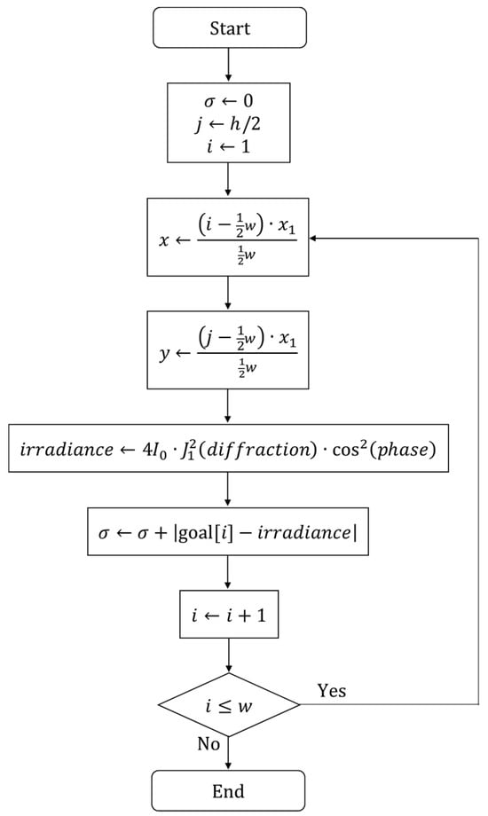
Figure 6. Algorithm 2. Fitness calculation algorithm.

4.3. Genetic Operators

As in any typical genetic algorithm, fitness evaluation is performed on phenotypes and genetic operators act on genotypes. Individuals are chosen by an elitist roulette selection Figure 7.

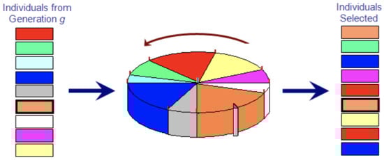
Figure 7. Roulette selection.

Roulette selection first assigns an expected value to each individual that is proportional to its fitness such that the sum of these values is equals to the population size. It works by creating a “roulette wheel” where each individual is assigned a slice of the wheel, and the size of the slice is determined by its fitness. When the wheel is spun, the individual whose slice aligns with the “marker” is selected. This is implemented by picking a random value in the range $[0,N]$ where N is the population size. It then sums up the expected values of all the individuals, and whatever individual causing the sum to exceed the random value is selected. This process is done $N-1$ times because the best individual is always preserved. In roulette selection, fitter individuals are more likely to pass to the next generation. Notice in Figure 7 that orange individual (the best solution) passes to the next generation at the same position because of the elitist algorithm. Moreover, orange, blue, red and yellow individuals had great odds to be selected (even more than once) for being acceptable solutions.

The crossover technique employed is two-point (see Figure 8). It is carried out between pairs of adjacent individuals $(i,i+1)$, where i is an even index $(0,2)$, and $i+1\ne$ best individual index. Checkpoints are random integer values in the range $[0\dots 31]$. This interval is due to the genotype is made up of thirty-two bits. The probability of crossover occurring has been set to $80\%$; this value usually ranges from $60\%$ to $90\%$. High values of crossover probability encourage search-space exploitation. In this work, we desire in most of the cases that new chromosomes, the offspring, to inherit good parts (bit sequences) of old chromosomes, maybe leading to better individuals. However, it is good practice to allow some part of the population to survive to the next generation.

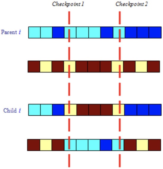
Figure 8. Two-point crossover; where dark colored genes store 1 (brown and blue) and light colored genes denote 0 (yellow and cyan).

The mutation technique is one-point uniform and consists of changing the value of a randomly selected bit from genotype i, as shown in Figure 9, where $i\ne$ best individual index. Mutation encourages search-space exploration [24], since it is made to prevent the algorithm from falling into local extreme, but it should not occur very often, because the genetic algorithm will in fact change to random search. This is way mutation probability has been set to $0.4$.

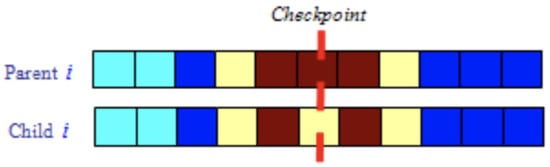
Figure 9. One-point uniform mutation; where dark colored genes store 1 (brown and blue) and light colored genes denote 0 (yellow and cyan).

5. Numerical Set-Up to Test the Algorithm

The employed parameters for this work are:

• Wavelength, ${\lambda }_0=0.000632$ mm (from a geometric point of view).
• Distance between observation plane and secondary sources $a=90$ mm.
• Distance from segments to beam splitter $\varphi =45$ mm.
• Separation between sources $d=0.1$ mm.
• Air index $n=1$.
• Size of observation plane in the x direction $=40$ mm.
• Maximum intensity $I_0=1024$.
• Apertures diameter $=2.0$ mm.

6. Results and Discussion

Figure 10 shows windows of a computer application, running under Linux, useful for generating Figure 10a,b to evaluate a Young pattern in *.fits format and to conserve fine details of the image, respectively. We can observe all the parameters involved in the generation of this image.

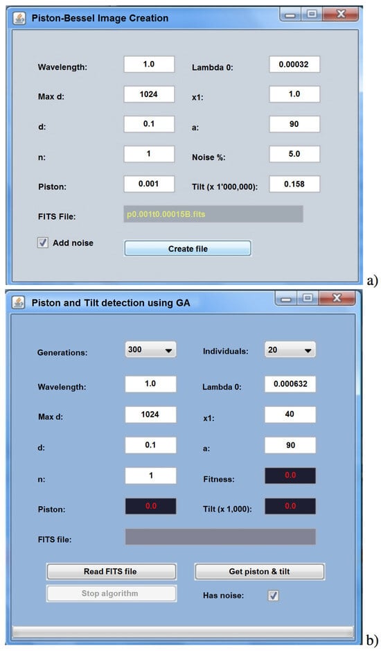
Figure 10. Application windows to (a) generate a Young pattern and (b) to evaluate an image with tilt and piston.

Figure 11 show a set of simulated images to be used in Young’s experiment for cophasing. An interesting area of these Young’s patterns is the central maximum where the interference fringes are changing due to misalignments for piston and tilt. We can notice that for the case of Figure 11a, the piston and tilt present at the same time in the pattern, and it produces a combined effect in the patterns. However, a small shift towards the right is observed in Figure 11b; this effect is an indicative of a variation in the initial phase of the produced pattern by a slight tilt. Furthermore, the pure effect of the piston is shown in Figure 11c, where a symmetric change in the fringes’ width is produced for the piston effect. These pattern width changes have been already reported in [15,17,21], and therefore, are again corroborated here.

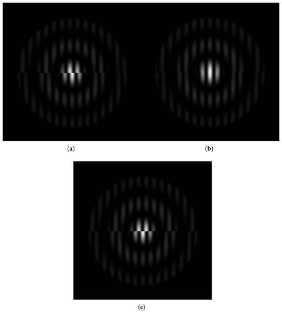
Figure 11. Young patterns images generated for the application with: (a) piston and tilt, (b) only tilt, and (c) only piston.

We decide it is suitable to analyze first the case when only piston or tilt are present separately.

First, we began by positioning the experiment in half of the total of the proposed numbers of generations G and individuals I; this is $(G,I)$. We realized that a work margin is necessary to realize three experiments of evaluation in the image, for $G>I$, with 2350 and 940 generations and individuals, respectively, and for $G<I$ (with $G=850$ and $I=1630$) and $G=I$ (for $G=1650$ and $I=1650$), as shown in Table 1, where $Exp(P_i,T_i)$, $Ext(P_i,T_i)$, $\%(P_i,T_i)$, and $(G,I)$ are the expected piston and tilt components, the extracted piston and tilt components, the accuracy percentage, and the generations and individuals obtained, respectively.

Table 1. Piston detection with GA and tilt = 0.

$\mathit{Exp}({\mathit{P}}_{\mathit{i}},{\mathit{T}}_{\mathit{i}})$	$\mathit{Ext}({\mathit{P}}_{\mathit{i}},{\mathit{T}}_{\mathit{i}})$	$\%({\mathit{P}}_{\mathit{i}},{\mathit{T}}_{\mathit{i}})$	$(\mathit{G},\mathit{I})$	Best-Fitness	Successful-Iterations
$(0.001,0.00)$	$(0.001,0.00)$	$(100,100)$	$(2350,940)$	$0.999937$	7 of 10

The main idea is to obtain the better number of $(G,I)$ where the GA shows an optimal behavior. For the case where the piston is only present ($tilt=0$), a piston percentage of $100\%$ was obtained, and for a piston of $0.001\approx 1.58\lambda$, with a best fitness of $0.999$ to realize 7 of 10 successful runs. We also realize experiments for $(G<I)$ and $(G=I)$ by finding the same precision parameters; however, the successful iterations number presents a progressive decrease, since it was obtained 5 and 6 of 10 successful iterations, respectively. Thus, the optimal number of $(G,I)$ was in the first interval, that is for $(G>I)$.

For the case when tilt is only present (piston = 0), we obtained a percentage of tilt of $100\%$ with a best fitness of $0.982443$ after to realize 10 of 10 successful iterations for $(G>I)$, see Table 2. In this case, we can notice that in 2 iterations a tilt of $0.000157$ mm $(\approx 0.248\lambda )$ was extracted, with a $99.367\%$ precision, a best fitness of $0.982442$, and an uncertainty of $0.623\%$. Through this, the cases for $(G<I)$ and for $(G=I)$ were not realized completely since the same tendency was observed for the two iterations of the first case $(G>I)$, where an uncertainty of $0.623\%$ was obtained.

Table 2. Tilt detection with GA and piston = 0.

$\mathit{Exp}({\mathit{P}}_{\mathit{i}},{\mathit{T}}_{\mathit{i}})$	$\mathit{Ext}({\mathit{P}}_{\mathit{i}},{\mathit{T}}_{\mathit{i}})$	$\%({\mathit{P}}_{\mathit{i}},{\mathit{T}}_{\mathit{i}})$	$(\mathit{G},\mathit{I})$	Best-Fitness	Successful-Iterations
$(0.0,0.000158)$	$(0.0,0.000158)$	$(100,100)$	$(2350,940)$	$0.982443$	10 of 10

Table 3 shows 10 iterations of piston and tilt detection by considering $50\%$ more of generations and individuals than in the cases of the previous tables. It can be noticed that in the second iteration the best fitness $0.999992$ has been obtained with an uncertainty of $0.02\%$ and $0.63\%$ for piston and tilt, respectively. Therefore, these values for piston and tilt could be considered as the best misalignments extracted. Other interesting cases are seen in iterations 7 and 8, where a similar fitness of $0.999989$ has been obtained. However, the precision was different in both cases, since a precision of $99.9988\%$ was obtained in the 7th iteration for a piston, with an uncertainty of $0.0012\%$ for the piston and for tilt a precision of $100\%$. For the 8th iteration, in the case of the piston the precision was $99.9997\%$, with an uncertainty of $0.0003\%$, and for the tilt a precision of $99.36708\%$, with an uncertainty of $0.632\%$. Furthermore, the average percentage of precision of piston detection with GA was obtained; it was $99.99479\%$, with an average uncertainty of $0.00521\%$, and for tilt an average precision of $99.620248\%$ was obtained with an average uncertainty of $0.3797\%$. This last results demonstrated that GA can obtain better results for the piston, when tilt is also present in the images (Figure 11).

Table 3. Piston and tilt detection with GA.

$\mathit{Exp}({\mathit{P}}_{\mathit{i}},{\mathit{T}}_{\mathit{i}})$	$\mathit{Ext}({\mathit{P}}_{\mathit{i}},{\mathit{T}}_{\mathit{i}})$	$\%({\mathit{P}}_{\mathit{i}},{\mathit{T}}_{\mathit{i}})$	$(\mathit{G},\mathit{I})$	Best-Fitness	# Iterations
$(1.0,0.000158)$	$(1.000028,0.000157)$	$(99.9972,99.36708)$	$(3550,1410)$	$0.999990$	1
$(1.0,0.000158)$	$(1.000002,0.000157)$	$(99.9998,99.36708)$	$(3550,1410)$	$0.999992$	2
$(1.0,0.000158)$	$(1.000102,0.000157)$	$(99.9898,99.36708)$	$(3550,1410)$	$0.999965$	3
$(1.0,0.000158)$	$(0.999993,0.000158)$	$(99.9993,100.0)$	$(3550,1410)$	$0.999989$	4
$(1.0,0.000158)$	$(1.000042,0.000157)$	$(99.9958,99.36708)$	$(3550,1410)$	$0.999966$	5
$(1.0,0.000158)$	$(1.000051,0.000158)$	$(99.9949,100.0)$	$(3550,1410)$	$0.999978$	6
$(1.0,0.000158)$	$(0.999988,0.000158)$	$(99.9988,100.0)$	$(3550,1410)$	$0.999989$	7
$(1.0,0.000158)$	$(1.000003,0.000157)$	$(99.9997,99.36708)$	$(3550,1410)$	$0.999989$	8
$(1.0,0.000158)$	$(1.000045,0.000158)$	$(99.9955,100.0)$	$(3550,1410)$	$0.999982$	9
$(1.0,0.000158)$	$(0.000031,0.000157)$	$(99.9969,99.36708)$	$(3550,1410)$	$0.999987$	10

7. Conclusions

We have developed a study of piston and tilt detection with GAs, where information about big pistons have been obtained, understanding big as in the order of some millimeters for the piston and for tilts of the order of some fractions of the wavelength. This simulated experiment has a minimum value of detection of $0.001$ mm ($1.52\lambda$ for the piston), since it was imposed for the mathematical models obtained by Young’s experiment to characterize the piston, which was initially non-linear and thus the dynamic detection range was bonded. Likewise the precision of the program to generate simulated images was adapted for this piston value as mentioned. In contrast, for tilt detection, the dynamic detection range could have been bigger than the piston dynamic range, since tilt in Young’s experiment exhibits linear behavior and was considered from 0 to ${\displaystyle \frac{\lambda }{2}}$. Thus, in this work, the dynamic detection ranges for piston and tilt with two segmented surfaces or panels were studied. Future work may include scaling up the simulation to support off-axis segmented mirrors and segmented surfaces with three panels.

References

- Chanan, G.; Troy, M.; Dekens, F.; Michaels, S.; Nelson, J.; Mast, T.; Kirkman, D. Phasing the mirror segments of the Keck telescopes: The broadband phasing algorithm. Appl. Opt. 1998, 37, 144–150. [Google Scholar] [CrossRef] [PubMed]
- Perera, S.; Pott, J.; Woillez, J.; Kulas, M.; Brandner, W.; Lacour, S.; Widmann, F. P-REx II. Off-line Performance on VLTI/GRAVITY. arXiv 2021, arXiv:2112.12837. [Google Scholar]
- Wang, B.; Jin, Z.; Dai, Y.; Yang, D.; Xu, F. Research on piston error sensing for segmented mirrors under atmospheric turbulence. Opt. Express 2023, 31, 33719–33731. [Google Scholar] [CrossRef]
- Rousseaux, T.; Primot, J.; Jaeck, J.; Rouzé, B.; Le Gall, C.; Bellanger, C. A piston and tilt wavefront sensor dedicated to the cophasing of segmented optics in low light level conditions. Opt. Lasers Eng. 2024, 181, 108412. [Google Scholar] [CrossRef]
- He, W.; Tian, X.; Guo, P.; Yu, T.; Yang, L.; Yang, Z.; Liu, Z. Co-phase detection of segmented mirrors based on optical vortex polarization phase-shifting interference. Opt. Commun. 2024, 569, 130614. [Google Scholar] [CrossRef]
- Qin, R.; Yin, Z.; Ke, Y.; Liu, Y. Large Piston Error Detection Method Based on the Multiwavelength Phase Shift Interference and Dynamic Adjustment Strategy. Photonics 2022, 9, 694. [Google Scholar] [CrossRef]
- Li, D.; Wang, D. High-Precision Piston Error Sensing of Segmented Telescope Based on Frequency Domain Filtering. IEEE Photonics J. 2024, 16, 6803506. [Google Scholar] [CrossRef]
- Guerra-Ramos, D.; Trujillo-Sevilla, J.; Rodríguez-Ramos, J.M. Global piston restoration of segmented mirrors with recurrent neural networks. OSA Contin. 2020, 3, 1355–1363. [Google Scholar] [CrossRef]
- Yue, D.; Xu, S.Y.; Nie, H.T.; Xu, B.Q.; Wang, Z.Y. A new hybrid algorithm for co-phasing segmented active optical system based on phase diversity. Optik 2016, 127, 985–990. [Google Scholar] [CrossRef]
- Wu, S.; Dong, J.; Xu, S.; Lu, Z.; Xu, B. Optimization of a segmented mirror with a global radius of curvature actuation system based on multi-fidelity surrogates. Optik 2021, 242, 166741. [Google Scholar] [CrossRef]
- Paykin, I.; Yacobi, L.; Adler, J.; Ribak, E.N. Phasing a segmented telescope. Phys. Rev. E 2015, 91, 023302. [Google Scholar] [CrossRef] [PubMed]
- Guillaume, A.; Terrile, R.J.; von Allmen, P. Fine alignment of the James Webb Space Telescope with a genetic algorithm. In Proceedings of the IEEE Aerospace Conference, Big Sky, MT, USA, 7–14 March 2009; Volume 7, pp. 1–7. [Google Scholar]
- Li, D.; Xu, S.; Wang, D.; Yan, D. Large-scale piston error detection technology for segmented optical mirrors via convolutional neural networks. Opt. Lett. 2019, 44, 1170–1173. [Google Scholar] [CrossRef]
- Bai, J.; Cheng, S.; Yang, G. Phase alignment of segmented mirrors using a digital wavefront interferometer. Opt. Eng. 1997, 36, 2355–2357. [Google Scholar] [CrossRef]
- Salinas-Luna, J.; Luna, E.; Salas, L.; Cruz-González, I.; Cornejo-Rodríguez, A. Ronchi test can detect piston by means of the defocusing term. Opt. Express 2004, 12, 3719–3736. [Google Scholar] [CrossRef] [PubMed]
- Malacara, D. Twyman-Green Interferometer. In Optical Shop Testing, 3rd ed.; Malacara, D., Ed.; Wiley-Interscience: Hoboken, NJ, USA, 2007; Chapter 2; pp. 46–96. [Google Scholar]
- Salinas-Luna, J.; Luna, E.; Salas, L.; Nunez, J. Experimental results on piston detection by using the classical Ronchi test. Appl. Opt. 2006, 45, 6990–6997. [Google Scholar] [CrossRef] [PubMed]
- Hopkins, H.H. Wave Theory of Aberrations, Wave and Ray Aberrations; The Claren-don Press: London, UK, 1950. [Google Scholar]
- Born, M.; Wolf, E. Principles of Optics, 7th ed.; Cambridge University Press: Cambridge, UK, 1999; pp. 290–292. [Google Scholar]
- Hecht, E. Optics, 5th ed.; Pearson Education: London, UK, 2017; pp. 473–476. [Google Scholar]
- Salinas-Luna, J.; Mentado Morales, J.; Nuñez-Alfonso, J.M. Lambda-shiftings for the secondary sources in the Young’s experiment allow to rebuild patterns looks like piston/tilt. Rev. Mex. Física E 2023, 20, 010207-1. [Google Scholar] [CrossRef]
- Holland, J.H. Adaptation in Natural and Artificial Systems. An Introductory Analysis with Applications to Biology, Control, and Artificial Intelligence; MIT Press Edition: Boston, MA, USA, 1992. [Google Scholar]
- Darwin, C. The Origin of Species. Means of Natural Selection, or the Preservation of Favoured Races in the Struggle for Life; D. Appleton and Company: New York, NY, USA, 1861. [Google Scholar]
- Spears, W.M. Crossover or Mutation? In Proceedings of the Second Workshop on Foundations of Genetic Algorithms, Vail, CO, USA, 26–29 July 1992; Volume 2, pp. 221–237. [Google Scholar]
Disclaimer/Publisher’s Note: The statements, opinions and data contained in all publications are solely those of the individual author(s) and contributor(s) and not of MDPI and/or the editor(s). MDPI and/or the editor(s) disclaim responsibility for any injury to people or property resulting from any ideas, methods, instructions or products referred to in the content. |
© 2025 by the authors. Licensee MDPI, Basel, Switzerland. This article is an open access article distributed under the terms and conditions of the Creative Commons Attribution (CC BY) license (https://creativecommons.org/licenses/by/4.0/).