Abstract
Innovation and technology are important tools for delivering efficiency and productivity improvement in the minerals sector. The uptake of technologies has proven to be an important lever for increasing the productivity of the mining sector. This paper provides a comprehensive analysis of mine-level productivity using global data of copper, gold, and platinum from 1991 to 2020. Various drivers of productivity have been analysed to draw policy insights. Empirical findings reveal significant disparities in terms of technical efficiency and productivity across mines and regions. The further decomposition of total factor productivity (TFP) into its different components suggests that the adoption of innovative practices and investment in technology adoption could improve the overall productivity of these commodities sectors. Our findings also suggest that an appropriate input mix and optimal scale of production could boost platinum mining productivity. Regional disparities in the productivity of different commodities sectors (e.g., South Africa vs. Zimbabwe) give policymakers insights into how to support production scale and productivity through appropriate input mixes.
1. Introduction
The mining industry’s productivity has steadily fallen over the last few decades [1,2,3]. These fluctuations in commodities sectors’ efficiency and productivity have presented challenges to global demand and supply balances. Mining exporting countries, in particular, are vulnerable to delayed growth due to low productivity [4,5,6]. The significant growth in resource demand caused by global industrialisation and urbanisation has put great pressure on mining companies to boost productivity. Industry leaders have primarily focused on using partial measures of productivity (e.g., labour productivity) as performance indicators, which do not fully reflect the factors underpinning their productivity [7,8]. Unlocking productivity potentials and studying alternatives for reversing falling trends are critical for a country’s economic success. The recent reduction in mining productivity has attracted the interest of policymakers and corporate executives.
Innovation in mining has been a key agenda for both mining businesses and policy makers. In recent years, the mining industry has focused on using innovation to increase productivity through a number of productivity-enhancing initiatives and technologies, such as mine automation, artificial intelligence (AI), and electric vehicles [1,9,10]. The advancements in technology (through the automation of processes) is increasing productivity by either maintaining the same workforce or directly reducing the number of employees required in production [11,12]. Conversely, the fall in ore quality across commodities as a result of the exploitation of low-quality resources is negating productivity improvements by increasing the costs of extraction and capital investment. Furthermore, the utilisation of input mixes and expansion in the scale of production have impacts on productivity patterns. The extent to which these varied elements influence production is still unknown. Therefore, it is critical to determine how all of these different elements explain the mining sector’s productivity.
Understanding the causes of productivity decline is difficult. Several factors influence mining industry productivity and efficiency, including management approaches, effective resource allocation, scale economies, and, most importantly, innovation [13]. Embracing new technologies and optimal management practices also significantly influences the efficiency and productivity of the mining industry [14]. Automation and advancements in robotics technology, for instance, contribute to decreases in carbon emissions and increases in mining industry productivity [10]. The development of technologies and their use in the mining industry have enhanced mineral recovery while lowering production costs and energy use [11].
This study examines the mining sector’s total factor productivity (TFP) and its drivers using a large mine-level panel dataset comprising copper, gold, and platinum. TFP is described as the increased in output level that cannot be explained by increases in inputs. In other words, it is simply regarded as the Solow residual or a result of technological improvements. We study numerous factors that explain the differences in efficiency and productivity between mines and other areas. The breakdown of TFP into its constituent parts provides useful policy insights into how to improve the mining sector’s performance.
The paper is structured as follows. Section 2 presents a review of the literature on TFP measurement and the components of its change. There is also a brief assessment of existing studies of mining sector productivity and their limitations. Section 3 goes into detail about the methods of measuring TFP and data that were used in the analysis. Section 4 discusses the results of TFP and its associated measures of efficiency change. Finally, Section 5 concludes with closing remarks and potential policy initiatives to increase mineral productivity.
2. Literature Review
The idea of productivity and its decomposition into its components, such as technical efficiency and allocative efficiency, was first introduced by Farrell his seminal work [15]. Farrell pointed out that a producer is always concerned with expanding the output level of the firm without using more resources. Excessive use of inputs for a given level of output or the production of less output from a given level of inputs results in technical inefficiency, while the inappropriate use of the mix of inputs leads to allocative inefficiency. After Farrell’s work, other measures were developed, including scale efficiency [16,17]. Technical efficiency is usually measured using either an input- or an output-oriented approach. Input-oriented technical efficiency is defined as the ability of a firm to minimize its input use to produce a given level of output (or hold output mixes fixed in the case of multiple outputs), while output-oriented technical efficiency is defined as the maximisation of output using a given level of inputs (or holding input mixes fixed in case of multiple inputs).
Researchers have attempted to understand the causes of declining productivity trends and examined the many variables that account for variations in mining performance. However, most of the existing literature has focused on partial productivity (such as labour) or aggregate-level productivity using residual approach [12,18,19,20]. Partial productivity (e.g., labour productivity) measures provide useful insights about a firm’s performance, but they can be limited in scope to providing an overall picture of the firm. On the other hand, the TFP and its associated measures of efficiency change can provide a comprehensive picture and identify areas that require improvement.
To examine productivity and its various drivers, researchers have widely used this approach in almost every field of economics and business. Researchers have made extensive use of data envelopment analysis (DEA) methods to compute the components of technical change and technical, allocative, and scale efficiency. Both input- and output-oriented approaches have been adopted to measure technical and allocative inefficiencies [21,22]. Applications range from agriculture [23,24,25] to manufacturing [2,26] and the services sector [27,28,29]. There are also other important drivers of TFP, including scale and scope economies and technical change, which need further investigation to identify comprehensive policy insights [13]. For instance, it would be interesting to know whether the uptake of technologies driving the productivity or scale and scope economies (as a result of appropriate output and input mixes) are important levers of TFP in the mining sector.
Over the past few decades, policy discussions have centered on the efficiency and productivity of the mining industry. Many studies have concentrated on the theoretical and empirical foundations of efficiency and productivity and relate these concepts to various factors, including innovation and technical change, the adoption of technologies, scale and scope economies, investment lags, capacity utilisation, and input quality [10,29,30]. However, most studies have examined the productivity of the mining sector using aggregate data [18,20,31,32,33]. For instance, Topp used data from the Australian mining industry to estimate productivity and find a downward trend in mining TFP between 2001–2002 and 2006–2007, concluding that the depletion of resources and capital adjustment contributed to the drop in TFP [33]. The analytical approach proposed by Grifell-Tatje and Lovell, on the other hand, divides changes in productivity into variations in capacity utilisation and price recovery. They pointed out that an analysis of Chile’s mining industry productivity by [34] using the Solow residual approach suggested that research and development (R&D) spending and technology appear to be important productivity drivers.
Other studies used either mine-level or aggregate data to investigate the efficiency and productivity of specific commodities [14,29,35]. de Solminihac et al., used the Solow residual approach to compute the TFP of the Chilean copper sector and concluded that the rising input costs and declining ore quality reduced labour productivity [34]. They also note a 42% decline in labour productivity from 1999 to 2010. Oliveira et al., used a limited dataset of 25 gold mining companies and noted a marginal improvement in environmental efficiency [36]. Some previous studies used global gold mine-level data for 2019 to estimate a carbon-adjusted efficiency and technology gap between different production environments and technologies, such as open pit and underground [12]. They noted significant disparities in efficiency (ranging from 18% to 100%) between mines, attributed to the technology gap.
Most of the available research on the mining industry’s productivity and efficiency is either constrained to TFP analyses at the aggregate level or uses sparse firm- and mine-level data. To identify numerous performance-enhancing factors, a thorough investigation of the mining sector’s productivity is required. It would be crucial to determine whether more resources should be devoted to R&D or innovation and technology adoption to increase productivity. This report attempts to offer a thorough overview of TFP and its significant drivers in the mining industry.
3. Methods and Data
Productivity is often implicitly measured as the ratio of an aggregate output to an aggregate input [37]. The aggregation of inputs and outputs must be performed using aggregators [13,38]. The identification of appropriate aggregator functions is important for the construction of various indexes. Both linear and non-linear aggregators can be used to construct TFP indexes. Linear aggregators have been widely used in cost minimisation or revenue maximisation estimations. The optimisation measures used in the economic literature typically use linear aggregators to estimate the components of TFP, for example, to minimize costs or maximize revenues/profits. However, the use of non-linear aggregators is uncommon in the productivity literature.
Productivity is defined as the ratio of an aggregate output to an aggregate input as follows:
where is an aggregate output, and is an aggregate input.
The of a firm between periods and can be defined as follows:
where and .
These indexes satisfy the axioms and tests, including monotonicity, linear homogeneity, proportionality, commensurability, and identity.
The decomposition of into its different components allows policymakers and researchers to identify the sources of growth of firms or industries. In the earlier literature, was defined as a measure of either technical change or ignorance using a growth accounting approach. The previous literature argued that technical change and the capital-to-labour ratio were the only sources of growth in output per head [37,39]. However, this interpretation has several limitations, as pointed out by Carlaw and Lipsey [40]. For instance, they point out that the aggregate measure of does not allow the identification of different sources of productivity change, whereas researchers and policymakers seek to understand the different drivers of productivity that could help to suggest appropriate policy measures. This paper decomposes into several measures, such as best practices and scale and scope economies. Different components of changes are defined and explained below.
3.1. Measures of Efficiency
TFP change can be decomposed into several components, such as technical change, technical, scale, mix efficiency change, and other measures of efficiency change (e.g., input- or output-scale mix efficiency) and have been discussed in the literature [13,38]. These components of TFP, as measures of efficiency, are briefly explained in Figure 1. For instance, F1F1 represents a restricted production frontier, where both input and output mixes are held fixed, whereas F2F2 represents the production frontier when both input and output mixes are allowed to change. represent the maximum possible aggregate output (on the restricted frontier), and maximum possible aggerate output with unrestricted production frontier), respectively, whereas represents the aggregate input quantity required to produce the aggregate output (), and represents the amount of minimum possible aggregate input that is producing the aggregate output (). Similarly, is the quantity of aggregate input that is required to produce maximum possible aggregate output () on the restricted frontier (F1F1), and is the amount of aggregate input that is required to produce maximum possible aggregate output () on the unrestricted frontier (F2F2). Point A shows that a mine is using an aggregate input Xnt to produce the output Qnt; however, the same level of output could be produced using a smaller amount of aggregate input (i.e., ). Any movement from point A to point B leads to increased TFP as a result of improvement in the input-oriented technical efficiency (i.e., In contrast, scale efficiency can be measured by moving around the frontier F1F1 from B to D (i.e., the ratio of slope of OB to slope OD). Now, if restrictions on input mixes are relaxed (i.e., shifting to new frontier F2F2), the mine can further reduce the aggregate input to produce the same output level Qnt, which is defined as input-oriented mix efficiency (i.e., A movement from point A to point E leads to an increase in the TFP of the mine, which can be decomposed into different components. We note that any movement from point D to point E measuring the slope (OU/OE) is defined as residual scale efficiency.
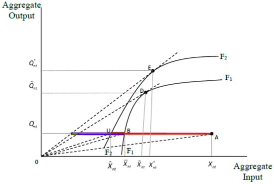
Figure 1.
Decomposition of TFP efficiency.
The input-oriented technical efficiency (ITE), which is based on the slope (OA/OB), is defined in terms the ratio of aggregate inputs as follows:
The input-oriented scale efficiency (ISE) is another measure commonly used to calculate efficiency related to economies/diseconomies of scale, identified using slope (OB/OD) as follows:
The input-oriented mix efficiency (IME), given by slope (OB/OU), is defined as follows:
Finally, the residual input-oriented scale efficiency (RISE) is shown in Equation (6). In other words, this is essentially a measure of scale efficiency, which may contain a residual mix effect or potential TFP change by relaxing restrictions on the input–output mix.
3.2. TFP and Its Decomposition
TFP efficiency (TFPE) is a useful overall measure of district performance, as shown in Equation (7). It is measured by the ratio of observed TFP to the maximum feasible TFP (TFP*), which, given the existing technology, is equal to slope (OA/OE). The TFP efficiency can provide the following meaningful decomposition.
When a mine transitions from a technically efficient point on the mix-restricted frontier to a point of maximum production on the unconstrained frontier, ISME measures the increase in TFP. Simply expressed, ISME, also known as the scale mix efficiency, quantifies the productivity gap caused by scale mix inefficiencies.
3.3. Empirical Model
A linear programming model based on DEA is used to estimate the measures of efficiency. Assuming that a locally linear production technology is used, we can write both input- and output-oriented production functions in linear form. An input-oriented locally linear production technology implies that any input vectors in the neighbourhood can be written in linear form as follows,
where μ and are non-negative, and may take any value. Since does not take any pre-assigned value, it exhibits variable returns to scale. It can exhibit local increasing returns to scale ( < 0), local decreasing returns to scale ( > 0), local non-increasing returns to scale ( ≥ 0), and local constant returns to scale ( = 0). The local input distance function corresponding to frontier (1) can be written as follows:
DEA involves choosing values of unknown parameters for minimizing the value of input distance Equation (9). Once the values of these parameters are selected using minimisation, one can identify the aggregate inputs and outputs parallel to different input and output vectors after performing some manipulations. DEA problems can be solved via either the primal or dual linear programming problem.
The dual input-oriented problem (for example) to choose optimum values is defined as follows:
3.4. Data and Variables
We use mine-level data for each mineral that has been obtained from S&P Global Market Intelligence’s reports on cost database. These data are standardised based on the year-end calendar. All production units are converted into a common scale extracted from the financial and technical reports of each company. It is possible that many mines have joint production of multiple commodities such as gold and copper, however, S&P Global provides cost of production data for each commodity separately, which has been downloaded directly from their website. Details about mine level data reporting methodology can be found at the following S&P website. The missing values for which information is unavailable are extrapolated using industry benchmarks and average values (such as productivity and energy consumption rates). All monetary data were denominated in US Dollars and derived in terms of unit costs. For further details, refer to the S&P Global Market Intelligence Database. Table 1 presents the descriptive statistics of output and input variables for all three commodities used in the TFP analysis. The variable log(y) is the logarithmic average quantity of each commodity produced per annum, whereas log(Ore) represents the logarithmic quantity of the ore bodies of each commodity used as an input in the production of minerals. However, labour, fuel, and capital inputs are presented in monetary terms, and logarithmic values are used in the production frontier.

Table 1.
Descriptive statistics of output and input quantities.
Figure 2 show the input cost trends from 1991 to 2020. As can be noted, there has been an upward trend in labour, energy, and capital costs since 2002. Copper mining is a capital-intensive industry, and for several reasons, such as diminishing ore grades and investments in technology, the capital costs involved have risen over time. Similarly, rising energy costs affect the sector’s efficiency and productivity. Figure 2a shows that in 2020, the energy cost of copper production was above 4 cents per pound. Similar trends can be observed in the input cost of gold production (See Figure 2b). However, platinum input costs show a different trend (as depicted in Figure 2c). It can be seen that this input cost rapidly declined until the 2000s; thereafter, capital costs remained stable, but both energy and labour costs fluctuated post-2009.
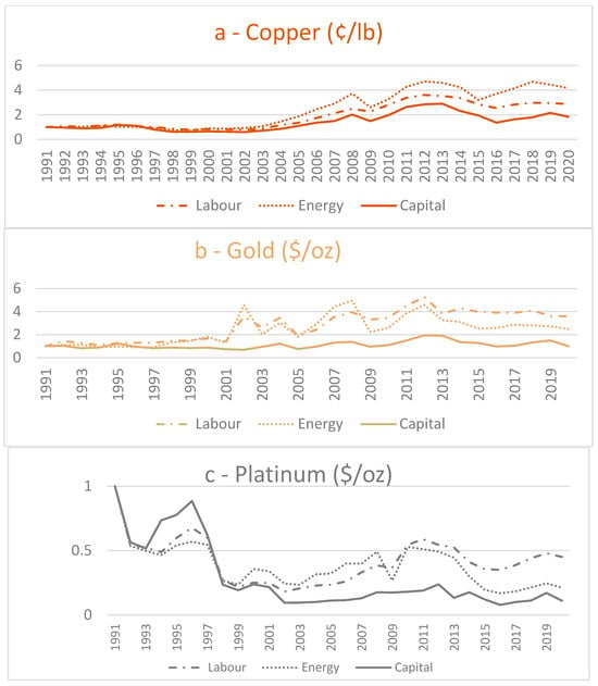
Figure 2.
(a–c) Input costs growth of selected commodities.
4. Empirical Results and Discussion
The data envelopment analysis (DEA) program was used with DPIN3.0 software to compute the TFP and its associated components, as indicated in Equations (2)–(8) and the graph. By addressing the linear programming issue outlined by O’Donnell, DEA computes the efficiency and other components of TFP [39]. We used the variable return to scale to calculate the input-oriented technical efficiency of each mine i in period t. To compute the efficiency estimates, we employed the primal input-oriented technique.
4.1. Technical Efficiency
Figure 3a–c depicts the technological efficiency distribution for copper, gold, and platinum. There are significant differences in efficiency across mines and areas for all three commodities. Estimates of mine-level technical efficiency reveal that copper mines are less efficient at transforming inputs into outputs on average. In other words, enterprises could have produced the same amount of output while using 40 percent less of their inputs. The considerable variation in technical efficiency across copper mines can be attributed to a number of factors, including ore quality, technologies, and mining practices. These disparities could be attributed to ore quality and technology differences adopted by different firms. A further examination of the mine-level efficiency of copper reveals that mines in Portugal and Saudi Arabia have the highest technical efficiency on average, whereas considerable mine-level dispersion is observed in Australia, Canada, and Laos (see, Table A1 in the Appendix A).
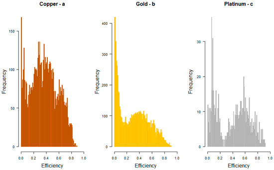
Figure 3.
(a–c) Distribution of technical efficiency of selected commodities.
Estimates of gold efficiency are provided in Figure 3b. It is noted that the distribution of efficiency appears to be more negatively skewed, since a huge number of mines demonstrate a low level of technical efficiency. A thorough examination of mine- and country-level data on technological efficiency finds significant variation at both the mine and regional levels. It has been observed that more efficient mines are located in African regions, which may be due to ore quality. However, a wide range of efficiency values was discovered in Ecuadorean, Bolivian, and Canadian mines. These findings are analogous to those of other researchers who discovered significant technological gaps between mines and locations [14]. Mines in the United States, Russia, and other locations, for example, have lower technical efficiency, which could be attributed to lower ore grade, as well as differing operating environments and technologies.
Platinum efficiency estimates show a similar scenario, albeit with a somewhat higher average technical efficiency. Figure 2c depicts the bimodal distribution of platinum mines’ efficiency, implying that mines are clustered at two points. Platinum’s average efficiency remains at 0.50, with individual results ranging from very low to highly efficient mines. Low mine efficiency may the result of several factors, such as geographic location, ore quality, and technology implementation. Mine size could also be another reason for the low efficiency of mines. There are many mines that produce a relatively small amount of platinum, which might have increased the cost of production and lowered the efficiency. For example, the most efficient platinum mines are located in the United States (0.91), followed by South Africa (0.87). Australian mines are likewise less technologically efficient. Global data also show that the most prolific mines are located in South Africa, which may be due to the ore quality, which makes those mines more efficient and productive. Due to price instability, the platinum industry has been under tremendous pressure to pursue cost-cutting and productivity-boosting strategies. These strategies can be accomplished by increasing output or reducing the quantity of resources consumed in order to boost productivity.
Figure 4a–c depicts a correlation analysis between productive capacity and technical efficiency to further explain the probable efficiency differentials between different platinum mines located in different localities. The logarithm of total production capacity (in tonnes) is depicted on the vertical axis, whereas the horizontal axis shows the technical efficiency (i.e., 0.00 to 1.00). At the national level, there is a strong correlation between production scale and efficiency. For example, copper mines (see Figure 4a) in Australia exhibit a significant association with scale operations, and technical efficiency means that greater mine operations may be the result of creative technology adoption. These patterns seem to be similar in all countries except China, which shows relatively larger dispersion in efficiency and production scales; hence, the Chinese results reflect weak correlation compared to mines located in other countries. The mine-level analysis in Canada, Chile, and South Africa yields similar results. However, it appears that these ties are weak in Chinese and US mining operations. The relationship between copper mine size and cost has been examined by many researchers [41,42,43]. However, there are mixed findings as to whether or not strong scale economies exist.
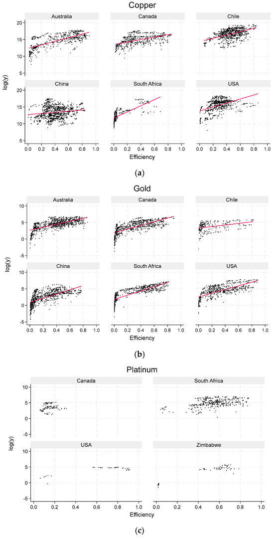
Figure 4.
(a–c) Relationship between technical efficiency and production scale.
The link between gold efficiency and production scales is depicted in Figure 4b. Gold mining, like copper mining, has a positive relationship between productive capacity and efficiency. However, unlike copper, the dispersion in gold mines’ efficiency has similar patterns in all countries. Mining operations’ efficiency can also be influenced by the different operating environments, such as open-pit and underground operations [44]. For instance, Ahmad et al., find that open-pit mines appear to be more efficient, perhaps due to the operations’ scales, which help to increase the mine-level productivity [14].
Figure 4c depicts the link between platinum mine output and efficiency. The findings show that the scale of production is positively connected to efficiency. Mining efficiency appears to have no favourable link with scale operations in most countries, except South Africa, where it shows a relatively positive correlation between production scales and efficiency. It notable that South Africa produces about 80% of the world’s platinum; hence, the country’s economy has a considerable impact on global supply.
4.2. Changes in Productivity and Its Drivers
TFP has been further analysed using global mine-level panel data from three commodities: copper, gold, and aluminium. The emphasis is on illustrating measures of efficiency change that explain the primary drivers of TFP. Figure 5 depicts the trend in TFP change for a selection of commodities.
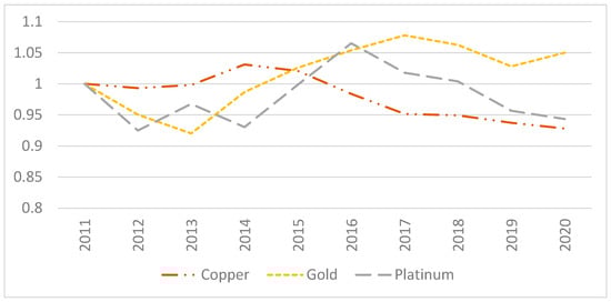
Figure 5.
TFP change in copper, gold, and platinum (2011–2020).
TFP trends show rises and falls across the timeframe, according to the results. For example, since 2013, there has been an upward trend in gold TFP change. Copper productivity, on the other hand, has been falling since 2014. Copper mining productivity may be declining indefinitely due to rising production costs. Platinum TFP, on the other hand, shows mixed patterns. Productivity increased until 2016, after which point it continuously dropped.
A further decomposition of productivity is depicted in Figure 6a–c. TFP was divided into two parts: technical efficiency change and scale mix efficiency change. While technical efficiency refers to best practices, scale mix efficiency refers to size and scope economies. In this industry, economies of scale and breadth are critical for determining effective market structures [45]. In reaction to pricing changes, businesses frequently alter the scale of their operations and/or the composition of their output and input mixtures. Significant losses in scale mix efficiency in Australia’s mining sector, for example, have been linked to increases in labour and capital utilisation over the last ten years. Due to these advances in input utilisation, sectoral trade terms have also improved. The appropriate course of action for the government will be determined based on whether rises in company profits are more or less significant than increases in productivity [38].
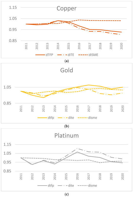
Figure 6.
(a–c) Decomposition of TFP into technical, scale, and mix efficiency.
Figure 6a describes the changes in copper TFP and associated measures of change, including technical efficiency and input scale mix efficiency change. While the change in input scale mix efficiency has been steady after 2016, there has been a continuous decline in TFP, which seems to be largely driven by technical efficiency. Figure 6b depicts the gold TFP and its associated components. It is noted that gold TFP has been increasing since 2013, with a slight dip in 2019. Scale and scope economies seem to contribute to TFP, whereas technical efficiency has been on decline. Platinum TFP and its associated components are presented in Figure 6c. Our results show that a change TFP is mainly explained through changes in technical efficiency, whereas scale mix efficiency shows a slight decline over time.
5. Conclusions
This paper examined the TFP and its various divers using global mine-level panel data of selected commodities (i.e., copper, gold, and platinum). We used rigorous methodologies to evaluate TFP and its associated components for people, miners, and organisations in various places. TFP and its components, such as technical efficiency and input-scale mix efficiency, were computed using a non-parametric approach. We use DPIN3.0 software to calculate exhaustive TFP measurements for commodity-level individual miners using the DEA technique. The main advantage of DEA is that it takes no functional form for the unknown technology. Furthermore, under this approach, (i) no specific assumptions for the error term are required, (ii) multiple input and output technologies can be estimated without any statistical issues (such as endogeneity), and (iii) its implementation is simple, requiring readily available computer software.
Empirical results show significant disparities in technical efficiency among mines across different commodities and regions. These differentials in efficiency may be the result of variation in technology adoption and the ore quality of the commodities under analysis. A further analysis of the decomposition of TFP into its different components identified the areas of improvement that could help to increase TFP. For instance, the copper, gold, and platinum sectors’ TFPs are mainly driven by technical efficiency, suggesting that the adoption of innovative practices and investment in technology adoption could improve the overall productivity of these commodities. In addition, the gold sector TFP is also explained by the input-scale mix efficiency to some extent, suggesting that appropriate input mix and optimum scale of production could improve the overall productivity of platinum mining. The findings also suggest that better capacity utilisation of mines and production scale could help to improve the mining sector’s productivity regarding the selected commodities.
To our knowledge, this is the first study that provides a detailed examination of commodity-level productivity and its primary drivers across three commodities. The findings imply that different operating circumstances and technical heterogeneity values have effects on mining productivity. New manufacturing techniques and technological advancements may help the mining sector to enhance output. Furthermore, differences in regional productivity and its determinants (e.g., South Africa vs. Zimbabwe) provide policymakers with insights on how to support scale and scope economies through optimal input mixes.
The current study did not investigate the technological gaps that could impede productivity across mines and regions. Future studies could investigate the technology gap within the mining sector and across regions. Furthermore, assessing environmental productivity trajectories could yield substantial policy consequences, particularly after controlling for greenhouse gas emissions, which is still on the study agenda for the future.
Funding
This research received no external funding.
Data Availability Statement
Data was downloaded from S&P Global website: https://www.capitaliq.spglobal.com/web/client?auth=inherit&OktaLogin=true#industry/mine (accessed on 31 March 2022).
Conflicts of Interest
The author declares no conflict of interest.
Appendix A
Table A1.
Copper efficiency.
Table A1.
Copper efficiency.
| Country | Mean | Std. Err. | Lower CI | Upper CI |
|---|---|---|---|---|
| Argentina | 0.339 | 0.024 | 0.292 | 0.386 |
| Armenia | 0.138 | 0.006 | 0.126 | 0.150 |
| Australia | 0.427 | 0.011 | 0.404 | 0.449 |
| Bolivia | 0.262 | 0.046 | 0.172 | 0.352 |
| Botswana | 0.258 | 0.034 | 0.193 | 0.324 |
| Brazil | 0.393 | 0.018 | 0.358 | 0.428 |
| Bulgaria | 0.357 | 0.015 | 0.328 | 0.386 |
| Canada | 0.385 | 0.009 | 0.366 | 0.403 |
| Chile | 0.416 | 0.006 | 0.404 | 0.429 |
| China | 0.373 | 0.004 | 0.364 | 0.381 |
| Dem. Rep. Congo | 0.699 | 0.007 | 0.684 | 0.713 |
| Dominican Republic | 0.032 | 0.004 | 0.025 | 0.039 |
| Ecuador | 0.370 | 0.000 | 0.370 | 0.370 |
| Eritrea | 0.532 | 0.068 | 0.399 | 0.665 |
| Finland | 0.462 | 0.024 | 0.416 | 0.508 |
| Indonesia | 0.468 | 0.018 | 0.432 | 0.504 |
| Iran | 0.555 | 0.014 | 0.528 | 0.582 |
| Kazakhstan | 0.417 | 0.018 | 0.381 | 0.452 |
| Kyrgyzstan | 0.436 | 0.010 | 0.417 | 0.455 |
| Laos | 0.599 | 0.038 | 0.524 | 0.674 |
| Mauritania | 0.481 | 0.040 | 0.403 | 0.560 |
| Mexico | 0.286 | 0.007 | 0.272 | 0.301 |
| Mongolia | 0.382 | 0.013 | 0.357 | 0.407 |
| Panama | 0.275 | 0.009 | 0.258 | 0.292 |
| Papua New Guinea | 0.445 | 0.022 | 0.401 | 0.489 |
| Peru | 0.318 | 0.008 | 0.302 | 0.334 |
| Philippines | 0.232 | 0.011 | 0.210 | 0.255 |
| Poland | 0.654 | 0.011 | 0.633 | 0.676 |
| Portugal | 0.736 | 0.015 | 0.707 | 0.766 |
| Russia | 0.566 | 0.012 | 0.542 | 0.590 |
| Saudi Arabia | 0.708 | 0.015 | 0.679 | 0.737 |
| South Africa | 0.093 | 0.008 | 0.078 | 0.108 |
| Spain | 0.428 | 0.030 | 0.369 | 0.487 |
| Sweden | 0.208 | 0.014 | 0.180 | 0.236 |
| Tanzania | 0.117 | 0.011 | 0.097 | 0.138 |
| Turkey | 0.756 | 0.009 | 0.738 | 0.774 |
| USA | 0.287 | 0.005 | 0.276 | 0.297 |
| Vietnam | 0.253 | 0.017 | 0.220 | 0.286 |
| Zambia | 0.584 | 0.009 | 0.567 | 0.601 |
| Zimbabwe | 0.059 | 0.004 | 0.052 | 0.066 |
Table A2.
Gold Efficiency.
Table A2.
Gold Efficiency.
| Country | Mean | Std. Err. | Lower CI | Upper CI |
|---|---|---|---|---|
| Argentina | 0.393 | 0.015 | 0.364 | 0.422 |
| Armenia | 0.262 | 0.017 | 0.229 | 0.296 |
| Australia | 0.395 | 0.007 | 0.381 | 0.409 |
| Bolivia | 0.410 | 0.063 | 0.286 | 0.534 |
| Brazil | 0.289 | 0.013 | 0.264 | 0.314 |
| Bulgaria | 0.191 | 0.028 | 0.136 | 0.247 |
| Burkina Faso | 0.499 | 0.014 | 0.471 | 0.527 |
| Canada | 0.291 | 0.009 | 0.274 | 0.307 |
| Chile | 0.182 | 0.013 | 0.156 | 0.208 |
| China | 0.223 | 0.006 | 0.211 | 0.235 |
| Cote d’Ivoire | 0.486 | 0.019 | 0.449 | 0.523 |
| Dem. Rep. Congo | 0.512 | 0.025 | 0.463 | 0.560 |
| Dominican Republic | 0.658 | 0.014 | 0.631 | 0.685 |
| Ecuador | 0.276 | 0.212 | 0.139 | 0.691 |
| Egypt | 0.503 | 0.015 | 0.474 | 0.533 |
| Eritrea | 0.266 | 0.103 | 0.064 | 0.467 |
| Finland | 0.215 | 0.022 | 0.171 | 0.258 |
| Ghana | 0.471 | 0.008 | 0.455 | 0.487 |
| Greece | 0.373 | 0.037 | 0.300 | 0.446 |
| Guatemala | 0.400 | 0.056 | 0.291 | 0.510 |
| Guinea | 0.488 | 0.020 | 0.449 | 0.527 |
| Guyana | 0.399 | 0.036 | 0.328 | 0.470 |
| Honduras | 0.292 | 0.024 | 0.246 | 0.338 |
| Indonesia | 0.502 | 0.022 | 0.459 | 0.546 |
| Iran | 0.017 | 0.001 | 0.015 | 0.019 |
| Kazakhstan | 0.274 | 0.017 | 0.240 | 0.307 |
| Kyrgyzstan | 0.493 | 0.040 | 0.415 | 0.571 |
| Laos | 0.225 | 0.025 | 0.176 | 0.273 |
| Liberia | 0.452 | 0.083 | 0.289 | 0.616 |
| Mali | 0.529 | 0.020 | 0.491 | 0.567 |
| Mauritania | 0.309 | 0.032 | 0.247 | 0.371 |
| Mexico | 0.201 | 0.006 | 0.189 | 0.213 |
| Mongolia | 0.198 | 0.047 | 0.106 | 0.291 |
| Namibia | 0.105 | 0.031 | 0.045 | 0.166 |
| New Zealand | 0.394 | 0.018 | 0.358 | 0.430 |
| Nicaragua | 0.499 | 0.021 | 0.458 | 0.541 |
| Panama | 0.032 | 0.004 | 0.024 | 0.039 |
| Papua New Guinea | 0.506 | 0.019 | 0.469 | 0.543 |
| Peru | 0.207 | 0.012 | 0.185 | 0.230 |
| Philippines | 0.284 | 0.020 | 0.244 | 0.325 |
| Poland | 0.015 | 0.002 | 0.011 | 0.018 |
| Russia | 0.375 | 0.011 | 0.354 | 0.396 |
| Saudi Arabia | 0.019 | 0.003 | 0.013 | 0.024 |
| Senegal | 0.545 | 0.029 | 0.488 | 0.603 |
| South Africa | 0.262 | 0.010 | 0.243 | 0.281 |
| Spain | 0.356 | 0.039 | 0.279 | 0.433 |
| Suriname | 0.464 | 0.026 | 0.413 | 0.515 |
| Sweden | 0.183 | 0.013 | 0.158 | 0.208 |
| Tajikistan | 0.338 | 0.036 | 0.267 | 0.410 |
| Tanzania | 0.597 | 0.015 | 0.568 | 0.627 |
| Thailand | 0.567 | 0.032 | 0.505 | 0.629 |
| Turkey | 0.503 | 0.017 | 0.470 | 0.536 |
| USA | 0.318 | 0.010 | 0.299 | 0.336 |
| Uzbekistan | 0.646 | 0.006 | 0.635 | 0.658 |
| Zambia | 0.078 | 0.003 | 0.072 | 0.085 |
| Zimbabwe | 0.029 | 0.002 | 0.025 | 0.032 |
References
- Matysek, A.L.; Fisher, B.S. Productivity and Innovation in the Mining Industry. BAE Research Report, Retrieved from Canberra. 2016. Available online: https://www.baeconomics.com.au/ (accessed on 7 November 2023).
- Chen, J.; Zhu, Z.; Xie, H.Y. Measuring intellectual capital: A new model and empirical study. J. Intellect. Cap. 2004, 5, 195–212. [Google Scholar] [CrossRef]
- Lala, A.; Moyo, M.; Rehbach, S.; Sellschop, R. Productivity in mining operations: Reversing the downward trend. AusIMM Bull. 2016, 2016, 46–49. Available online: https://www.ausimm.com/bulletin (accessed on 7 November 2023).
- Duan, L. Estimation of export cutoff productivity of Chinese industrial enterprises. PLoS ONE 2022, 17, e0277842. [Google Scholar] [CrossRef]
- Weldegiorgis, F.S.; Dietsche, E.; Ahmad, S. Inter-Sectoral Economic Linkages in the Mining Industries of Botswana and Tanzania: Analysis Using Partial Hypothetical Extraction Method. Resources 2023, 12, 78. [Google Scholar] [CrossRef]
- Yasmin, T.; El Refae, G.A.; Eletter, S.; Kaba, A. Examining the total factor productivity changing patterns in Ka-zakhstan: An input-output analysis. J. East. Eur. Cent. Asian Res. JEECAR 2022, 9, 938–950. [Google Scholar]
- Fernandez, V. Copper mining in Chile and its regional employment linkages. Resour. Policy 2021, 70, 101173. [Google Scholar] [CrossRef]
- Garcia, P.; Knights, P.F.; Tilton, J.E. Labor productivity and comparative advantage in mining: The copper industry in Chile. Resour. Policy 2001, 27, 97–105. [Google Scholar] [CrossRef]
- Gruenhagen, J.H.; Parker, R. Factors driving or impeding the diffusion and adoption of innovation in mining: A systematic review of the literature. Resour. Policy 2020, 65, 101540. [Google Scholar] [CrossRef]
- Humphreys, D. Mining productivity and the fourth industrial revolution. Miner. Econ. 2020, 33, 115–125. [Google Scholar] [CrossRef]
- Sánchez, F.; Hartlieb, P. Innovation in the Mining Industry: Technological Trends and a Case Study of the Challenges of Disruptive Innovation. Min. Met. Explor. 2020, 37, 1385–1399. [Google Scholar] [CrossRef]
- Lovell, C.A.K.; Lovell, J.E. Productivity decline in Australian coal mining. J. Prod. Anal. 2013, 40, 443–455. [Google Scholar] [CrossRef]
- Ahmad, S. Estimating input-mix efficiency in a parametric framework: Application to state-level agricultural data for the United States. Appl. Econ. 2020, 52, 3976–3997. [Google Scholar] [CrossRef]
- Ahmad, S.; Steen, J.; Ali, S.; Valenta, R. Carbon-adjusted efficiency and technology gaps in gold mining. Resour. Policy 2023, 81, 103327. [Google Scholar] [CrossRef]
- Farrell, M.J. The Measurement of Productive Efficiency. J. R. Stat. Soc. Ser. A Gen. 1957, 120, 253–290. [Google Scholar] [CrossRef]
- Färe, R.; Grosskopf, S.; Norris, M.; Zhang, Z. Productivity Growth, Technical Progress, and Efficiency Change in Industrialized Countries. Am. Econ. Rev. 1994, 84, 66–83. [Google Scholar]
- Nishimizu, M.; Page, J.M. Total Factor Productivity Growth, Technological Progress and Technical Efficiency Change: Dimensions of Productivity Change in Yugoslavia, 1965–1978. Econ. J. 1982, 92, 920–936. [Google Scholar] [CrossRef]
- Mahadevan, R.; Asafu-Adjaye, J. The productivity–inflation nexus: The case of the Australian mining sector. Energy Econ. 2005, 27, 209–224. [Google Scholar] [CrossRef]
- Parida, M.; Madheswaran, S. Effect of firm ownership on productivity: Empirical evidence from the Indian mining industry. Miner. Econ. 2021, 34, 87–103. [Google Scholar] [CrossRef]
- Syed, A.; Grafton, R.Q.; Kalirajan, K.; Parham, D. Multifactor productivity growth and the Australian mining sector. Aust. J. Agric. Resour. Econ. 2015, 59, 549–570. [Google Scholar] [CrossRef]
- Charnes, A.; Cooper, W.W.; Rhodes, E. Measuring the efficiency of decision making units. Eur. J. Oper. Res. 1978, 2, 429–444. [Google Scholar] [CrossRef]
- Schmidt, P.; Lovell, C.K. Estimating technical and allocative inefficiency relative to stochastic production and cost frontiers. J. Econ. 1979, 9, 343–366. [Google Scholar] [CrossRef]
- Ahmad, S.; Shankar, S.; Steen, J.; Verreynne, M.-L.; Burki, A.A. Using measures of efficiency for regionally-targeted smallholder policy intervention: The case of Pakistan’s horticulture sector. Land Use Policy 2021, 101, 105179. [Google Scholar] [CrossRef]
- Bravo-Ureta, B.E.; Pinheiro, A.E. Technical, Economic, and Allocative Efficiency in Peasant Farming: Evidence from the Dominican Republic. Dev. Econ. 1997, 35, 48–67. [Google Scholar] [CrossRef]
- Kalirajan, K.P. On measuring economic efficiency. J. Appl. Econom. 1990, 5, 75–85. [Google Scholar] [CrossRef]
- Ahmad, S.; Burki, A.A. Banking deregulation and allocative efficiency in Pakistan. Appl. Econ. 2016, 48, 1182–1196. [Google Scholar] [CrossRef]
- Burki, A.A.; Ahmad, S. Bank governance changes in Pakistan: Is there a performance effect? J. Econ. Bus. 2010, 62, 129–146. [Google Scholar] [CrossRef]
- Drake, J.; Swisdak, M.; Che, H.; Shay, M. Electron acceleration from contracting magnetic islands during reconnec-tion. Nature 2006, 443, 553–556. [Google Scholar] [CrossRef]
- Fukuyama, H.; Weber, W.L. Estimating output allocative efficiency and productivity change: Application to Japanese banks. Eur. J. Oper. Res. 2002, 137, 177–190. [Google Scholar] [CrossRef]
- Isaiah, M.; Johane, D.; Dambala, G.; Fiona, T. Environmental and Technical Efficiency in Large Gold Mines in Developing Countries. MPRA Paper. 2021. Available online: https://ideas.repec.org/p/pra/mprapa/108068.html (accessed on 7 November 2023).
- Shao, L.; He, Y.; Feng, C.; Zhang, S. An empirical analysis of total-factor productivity in 30 sub-sub-sectors of China’s nonferrous metal industry. Resour. Policy 2016, 50, 264–269. [Google Scholar] [CrossRef]
- Grifell-Tatjé, E.; Lovell, C.A.K. Productivity, price recovery, capacity constraints and their financial consequences. J. Prod. Anal. 2014, 41, 3–17. [Google Scholar] [CrossRef][Green Version]
- Topp, V. Productivity in the Mining Industry: Measurement and Interpretation; productivity commission staff working paper; Australian Productivity Commission: Canberra, Australia, 2008. [Google Scholar]
- Ilboudo, P.S. Foreign Direct Investment and Total Factor Productivity in the Mining Sector: The Case of Chile; Connecticut College: New London, CT, USA, 2014. [Google Scholar]
- De Solminihac, H.; Gonzales, L.E.; Cerda, R. Copper mining productivity: Lessons from Chile. J. Policy Model. 2018, 40, 182–193. [Google Scholar] [CrossRef]
- Oliveira, R.; Camanho, A.S.; Zanella, A. Expanded eco-efficiency assessment of large mining firms. J. Clean. Prod. 2017, 142, 2364–2373. [Google Scholar] [CrossRef]
- Jorgenson, D.W.; Griliches, Z. The Explanation of Productivity Change. Rev. Econ. Stud. 1967, 34, 249–283. [Google Scholar] [CrossRef]
- O’Donnell, C.J. Nonparametric Estimates of the Components of Productivity and Profitability Change in U.S. Agriculture. Am. J. Agric. Econ. 2012, 94, 873–890. [Google Scholar] [CrossRef]
- Solow, R.M. Technical Change and the Aggregate Production Function. Rev. Econ. Stat. 1957, 39, 312. [Google Scholar] [CrossRef]
- Carlaw, K.I.; Lipsey, R.G. Productivity, Technology and Economic Growth: What is the Relationship? J. Econ. Surv. 2003, 17, 457–495. [Google Scholar] [CrossRef]
- Crowson, P. Mine size and the structure of costs. Resour. Policy 2003, 29, 15–36. [Google Scholar] [CrossRef]
- Bozorgebrahimi, A.; Hall, R.A.; Morin, M.A. Equipment size effects on open pit mining performance. Int. J. Surf. Min. Reclam. Environ. 2005, 19, 41–56. [Google Scholar] [CrossRef]
- Yatchew, A. An elementary estimator of the partial linear model. Econ. Lett. 1997, 57, 135–143. [Google Scholar] [CrossRef]
- Kulshreshtha, M.; Parikh, J.K. Study of efficiency and productivity growth in opencast and underground coal mining in India: A DEA analysis. Energy Econ. 2002, 24, 439–453. [Google Scholar] [CrossRef]
- Triebs, T.P.; Saal, D.S.; Arocena, P. Estimating economies of scale and scope with flexible technology. J. Prod. Anal. 2016, 45, 173–186. [Google Scholar] [CrossRef]


Disclaimer/Publisher’s Note: The statements, opinions and data contained in all publications are solely those of the individual author(s) and contributor(s) and not of MDPI and/or the editor(s). MDPI and/or the editor(s) disclaim responsibility for any injury to people or property resulting from any ideas, methods, instructions or products referred to in the content. |
© 2023 by the author. Licensee MDPI, Basel, Switzerland. This article is an open access article distributed under the terms and conditions of the Creative Commons Attribution (CC BY) license (https://creativecommons.org/licenses/by/4.0/).