Kangaroos in Cambridge ^†

Abstract

In this tutorial paper the Gull–Skilling kangaroo problem is revisited. The problem is used as an example of solving an under-determined system by variational principles, the maximum entropy principle (MEP), and Information Geometry. The relationship between correlation and information is demonstrated. The Kullback–Leibler divergence of two discrete probability distributions is shown to fail as a distance measure. However, an analogy with rigid body rotations in classical mechanics is motivated. A table of proper “geodesic” distances between probability distributions is presented. With this paper the authors pay tribute to their late friend David Blower.

1. Introduction

On my (RB) first meeting with Dr. John Skilling and Dr. Steve Gull in Cambridge in 1987, I was posed the following problem [1,2,3]:

In Australia, $3/4$ of the kangaroos are right-handed and $1/3$ have blue eyes. Can you construct the $2\times 2$ probability table?

Having no clue about the use of their shorter forelegs, let alone any handedness, nor of the colour of their eyes, I assumed that:

• a kangaroo is right-handed or left-handed; and
• a kangaroo has blue eyes or green eyes.

This means that there are four distinct possibilities: right-handed with blue eyes, right-handed with green eyes, left-handed with blue eyes, and left-handed with green eyes. The statement space is of dimension 2 × 2 and has 4 cells, and a bare probability table looks like Table 1, showing the two given marginal values and the sum.

Table 1. Probability table: version 1.

Probability Table
	Blue eyes	Green eyes
Right-handed			$3/4$
Left-handed
	$1/3$		1

The two other marginal values result from normalizing the sum of the joint probabilities. Filling in the table a little more, we obtain Table 2. The notation $Q_i$ for probabilities originates with David Blower, who avoids the overused P-symbol. In this paper we follow Blower’s notation closely [4].

Table 2. Probability table: version 2.

Probability Table
	Blue eyes	Green eyes
Right-handed	$Q_1$	$Q_2$	$3/4$
Left-handed	$Q_3$	$Q_4$	$1/4$
	$1/3$	$2/3$	1

I thought about this problem for a short while and filled in the table by multiplying the row and column marginal values, as in Table 3.

Table 3. Probability table, version 3.

Probability Table
	Blue eyes	Green eyes
Right-handed	$1/4$	$1/2$	$3/4$
Left-handed	$1/12$	$1/6$	$1/4$
	$1/3$	$2/3$	1

However, then I was presented with the following set of equations

$$\begin{array}{cc}\hfill Q_1+Q_2& =3/4\hfill \\ \hfill Q_1+Q_3& =1/3\hfill \\ \hfill Q_1+Q_2+Q_3+Q_4& =1.\hfill \end{array}$$

(1)

There are only three equations in four unknowns, leaving any other (consistent) equations relating to the $Q_i$ redundant. This is an under-determined system. In my proposed solution, I must have used a fourth equation. So, where did this fourth equation come from? My answer was that I assumed that handedness and eye colour are independent, and thus the marginal probabilities could be multiplied. “Aah”, they said, “you have applied the Maximum Entropy Principle!”

Jaynes discussed and extended the kangaroo problem in the Fourth Maximum Entropy Workshop in 1984 [3].

This under-determined system has one free variable. Choosing $Q_1$ as the free variable, the equations reduce to

$$\begin{array}{cc}\hfill Q_2& =3/4-Q_1\hfill \\ \hfill Q_3& =1/3-Q_1\hfill \\ \hfill Q_4& =-1/12+Q_1.\hfill \end{array}$$

(2)

A symbolic solution can be obtained by using Wolfram Mathematica’s Reduce[] function [5] as shown in Figure 1.

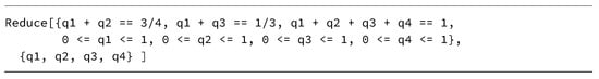
Figure 1. Wolfram Mathematica code for solving the under-determined problem (2).

In this code snippet, the three equations can be recognized as well as the positivity condition. The solution is

$$1/12\le Q_1\le 1/3.$$

(3)

With this solution the probability table can be filled in as in Table 4.

Table 4. Probability table, version 4.

Probability Table
	Blue eyes	Green eyes
Right-handed	$1/12\le Q_1\le 1/3$	$3/4-Q_1$	$3/4$
Left-handed	$1/3-Q_1$	$-1/12+Q_1$	$1/4$
	$1/3$	$2/3$	1

Figure 2 shows a range of solutions to this problem. This figure illustrates the correlation and anti-correlation between the various $Q_i$-s. Since $Q_1$and $Q_2$ have to maintain their sum as $3/4$, they must be anti-correlated. Therefore the coloured lines cross each other between $Q_1$ and $Q_3$. Similarly, $Q_1$ is anti-correlated with $Q_3$. Therefore, $Q_2$ and $Q_3$ have to be correlated, and the coloured lines between them do not cross. Finally, $Q_1$ is correlated with $Q_4$, which can be seen from the repeated $Q_1$-axis at the right.

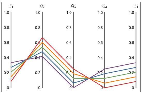
Figure 2. Parallel-axis plot of the $Q_1$, $Q_2$, $Q_3$, and $Q_4$, for $Q_1$ between $1/12$ (red) and $1/3$ (purple) in equidistant steps of $1/16$. For clarity, the $Q_1$ axis is repeated on the right.

2. Variational Principles

A possible solution for an under-determined problem can be found by adopting a variational principle. This is a function of the joint probabilities to be optimized (maximized or minimized) under some constraints, whose free parameters correspond to the missing equations. Sivia considers four variational functions: the entropy, the sum of squares, the sum of logarithms, and the sum of square roots, as shown in Table 5 [1].

Table 5. Sivia’s four variational functions: entropy, sum of squares, sum of logarithms, sum of square roots.

2cVariational Functions
	Function
Maximum entropy	$-{\sum }_{i=1}^n{Q}_{i}log{Q}_i$
Least squares	${\sum }_{i=1}^n{Q}_i^2$
Maximum logarithms	${\sum }_{i=1}^{n}log{Q}_i$
Maximum square roots	${\sum }_{i=1}^n\sqrt{Q_i}$

In the case of the Least Squares variational function we have

$$\begin{array}{cc}\hfill 31f\left(Q\right)& =Q_1^2+Q_2^2+Q_3^2+Q_4^2\hfill \\ \hfill & =Q_1^2+{\left(3/4-Q_1\right)}^2+{\left(1/3-Q_1\right)}^2+{\left(-1/12+Q_1\right)}^2\hfill \\ \hfill & =4Q_1^2-7/3Q_1+49/72.\hfill \end{array}$$

(4)

This is a quadratic function and has a unique minimum at

$$Q_1=7/24,$$

(5)

which yields the exact solution of $M_{\mathrm{VP},\mathrm{LeastSq}}$

$$Q_i=(7/24,11/24,1/24,5/24).$$

(6)

For the Maximum Entropy, the variational function

$$f\left(Q\right)=-Q_{1}log{Q}_1-Q_{2}log{Q}_2-Q_{3}log{Q}_3-Q_{4}log{Q}_4$$

(7)

has to be maximized, subject to the constraints. This function has a unique maximum at

$$Q_1=1/4,$$

(8)

which yields the exact solution of $M_{\mathrm{VP},\mathrm{MaxEnt}}$

$$Q_i=(1/4,1/2,1/12,1/6).$$

(9)

The solutions for $Q_1$ for the Maximum logarithms and Maximum square roots variational equations only can be obtained via numerical optimization. For each solution $Q_1$, the other three $Q_i$ values follow directly from (2). The Variational Principle solutions are tabulated in Table 6 and visualized in Figure 3.

Table 6. The Variational Principle solutions.

Variational Functions
Model	Function	$Q_i$
$M_{\mathrm{VP},\mathrm{MaxEnt}}$	$-{\sum }_{i=1}^n{Q}_{i}log{Q}_i$	$(0.25,0.50,0.08,0.17)$
$M_{\mathrm{VP},\mathrm{LeastSq}}$	${\sum }_{i=1}^n{Q}_i^2$	$(0.29,0.46,0.04,0.21)$
$M_{\mathrm{VP},\mathrm{MaxLog}}$	${\sum }_{i=1}^{n}log{Q}_i$	$(0.23,0.52,0.11,0.14)$
$M_{\mathrm{VP},\mathrm{MaxSqrt}}$	${\sum }_{i=1}^n\sqrt{Q_i}$	$(0.24,0.51,0.10,0.15)$

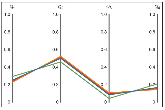
Figure 3. Parallel axis plot of the Variational Principle solutions: $M_{\mathrm{VP},\mathrm{MaxEnt}}$ is blue, $M_{\mathrm{VP},\mathrm{LeastSq}}$ is green, $M_{\mathrm{VP},\mathrm{MaxLogs}}$ is orange, and $M_{\mathrm{VP},\mathrm{MaxSqrt}}$ is red.

However, given these four different solutions to the kangaroo problem, we need a rationale for choosing one of them. Which one is ’best’? Sivia states that barring some evidence about a gene-linkage between handedness and eye colour for kangaroos, the MaxEnt model is preferred because this model provides the only uncorrelated assignment of the $Q_i$. This is shown in Section 4.

3. State Space and Constraint Functions

In the kangaroo problem, we have two traits: handedness and eye colour. Each trait has a set of features; for the handedness they are “right-handed” and “left-handed”; for the eye colour “blue” and “green”. Mixtures of features are not allowed. Therefore, for every trait, one, and only one, feature applies; the features are mutually exclusive.

More abstractly, the features can be represented as statements. The combined features from different traits form joint statements. The joint statements define a state space of dimension $n=4$. The n cells uniquely number the joint statements. Table 7 shows the general setup.

Table 7. The n cells of the state space uniquely number the joint statements.

State Space Table
	Blue eyes	Green eyes
Right-handed	$\left(X=x_1\right)$	$\left(X=x_2\right)$	$3/4$
Left-handed	$\left(X=x_3\right)$	$\left(X=x_4\right)$	$1/4$
	$1/3$	$2/3$	1

Any joint statement about a kangaroo can be placed in one and only one cell of the state space. For example, a left-handed and blue-eyed kangaroo is uniquely defined by the joint statement $\left(X=x_3\right)$. In this notation, the X denotes the two traits, and the $x_3$ specifies the features in cell 3. The state space is congruent to the probability table of Table 1, but it has a different role. The joint statements, $\left(X=x_i\right)$, are logical statements which can be either True or False.

A constraint function is defined over the state space, as shown in Table 8. The function F assigns a Boolean value to each joint statement and returns a vector of values ([4], Ch. 21)

$$\left(F\left(X=x_1\right),F\left(X=x_2\right),F\left(X=x_3\right),F\left(X=x_4\right)\right).$$

(10)

The constraint function vector specifies the operation of a constraint.

Table 8. The constraint function $F\left(X=x_i\right)$ is a function defined on the space of joint statements.

State Space Table
	Blue eyes	Green eyes
Right-handed	$F\left(X=x_1\right)$	$F\left(X=x_2\right)$	$3/4$
Left-handed	$F\left(X=x_3\right)$	$F\left(X=x_4\right)$	$1/4$
	$1/3$	$2/3$	1

The constraint function $F_1$ for our first constraint, “In Australia $3/4$ of the kangaroos are right-handed ...,” is shown in Table 9. Writing out the constraint function vector for $F_1$, we have

$$\left(F_1\left(X=x_1\right),F_1\left(X=x_2\right),F_1\left(X=x_3\right),F_1\left(X=x_4\right)\right)=(1,1,0,0).$$

(11)

The corresponding constraint function vector for the left-handed kangaroos is its complement, $(0,0,1,1)$.

Table 9. The constraint function $F_1$ for the constraint “$3/4$ of the kangaroos are right-handed.”

State Space Table
	Blue eyes	Green eyes
Right-handed	$F_1\left(X=x_1\right)=1$	$F_1\left(X=x_2\right)=1$	$3/4$
Left-handed	$F_1\left(X=x_3\right)=0$	$F_1\left(X=x_4\right)=0$	$1/4$
	$1/3$	$2/3$	1

The constraint function $F_2$ for the second constraint, “... and $1/3$ have blue eyes,” is shown in Table 10. Writing out the constraint function vector $F_2$, we obtain

$$\left(F_2\left(X=x_1\right),F_2\left(X=x_2\right),F_2\left(X=x_3\right),F_2\left(X=x_4\right)\right)=(1,0,1,0).$$

(12)

The constraint function vector for the blue-eyed kangaroos is $(1,0,1,0)$, and $(0,1,0,1)$ for the green-eyed ’roos.

Table 10. The constraint function vector for the second constraint ($1/3$ of the kangaroos have blue eyes).

State Space Table
	Blue eyes	Green eyes
Right-handed	$F_2\left(X=x_1\right)=1$	$F_2\left(X=x_2\right)=0$	$3/4$
Left-handed	$F_2\left(X=x_3\right)=1$	$F_2\left(X=x_4\right)=0$	$1/4$
	$1/3$	$2/3$	1

The probability distribution is normalized, which means that the sum of all joint probabilities is unity. This is also a constraint. The overall normalization is a universal constraint function vector

$$\left(F_0\left(X=x_1\right),F_0\left(X=x_2\right),F_0\left(X=x_3\right),F_0\left(X=x_4\right)\right)=(1,1,1,1).$$

(13)

This whole business of creating constraint function vectors for assigning probabilities may seem overly elaborate but conceptually, and operationally, we need a way to connect a statement$\left(X=x_i\right)$ with a numerical value. Technically, F is an operator that accepts a joint statement as its variable and returns a Boolean value. Furthermore, the constraint function vectors $F_j$ become the basis vectors ${\mathbf{e}}_j$ in the vector space of the information geometry in Section 6.

4. Correlation, Covariance, and Entropy

What do correlation and covariance actually mean, and what is the difference? Sometimes the two terms are used interchangeably.

We all have an intuitive interpretation. For instance, people’s heights and weights are correlated, which means that generally, tall persons weigh more than short ones. The two variables vary together; they are co-varying. However, this does not necessarily reflect a causal relationship. Gaining weight does not automatically imply becoming taller, as we all know.

4.1. Expectation

Suppose that a function $V\left(X=x_i\right)$ is defined over the state space and returns a numerical value for each joint statement. The expectation of V is

$$⟨V⟩=\sum _{i=1}^{n}V\left(X=x_i\right)Q_i.$$

(14)

The sum is over all $V\left(X=x_i\right)$ values in the state space, whereas the $Q_i$ are from the probability table. The expectation value, $⟨V⟩$, is a numerical quantity.

With this definition, let’s compute the expectation for “right-handedness”. The constraint function vector for right-handedness, $F_1=(1,1,0,0)$, acts as the quantity V

$$\begin{array}{cc}\hfill ⟨F_1⟩& =\sum _{i=1}^n{F}_1\left(X=x_i\right)Q_i\hfill \\ \hfill & =F_1\left(X=x_1\right)Q_1+F_1\left(X=x_2\right)Q_1+F_1\left(X=x_3\right)Q_1+F_1\left(X=x_4\right)Q_1\hfill \\ \hfill & =1Q_1+1Q_2+0Q_3+0Q_4\hfill \\ \hfill & =Q_1+Q_2\hfill \\ \hfill & =3/4.\hfill \end{array}$$

(15)

In the last step, we have used the information given in Table 2. The expectation for right-handedness thus equals its marginal value.

Similarly for “blue eyes”, with $F_2=(1,0,1,0)$

$$\begin{array}{cc}\hfill ⟨F_2⟩& =\sum _{i=1}^n{F}_2\left(X=x_i\right)Q_i\hfill \\ \hfill & =1Q_1+0Q_2+1Q_3+0Q_4\hfill \\ \hfill & =Q_1+Q_3\hfill \\ \hfill & =1/3.\hfill \end{array}$$

(16)

Furthermore, the expectation value for blue eyes again equals its marginal value.

4.2. Variance

The variance of the $V\left(X=x_i\right)$ values is defined as

$$\begin{array}{cc}\hfill \mathrm{var}\left(V\right)& =\sum _{i=1}^n{\left(V\left(X=x_i\right)-⟨V⟩\right)}^2{Q}_i\hfill \\ \hfill & =⟨{\left(V\left(X=x_i\right)-⟨V⟩\right)}^2⟩.\hfill \end{array}$$

(17)

Notice that there are two nested sets of brackets $⟨.⟩$ involved. The $⟨V⟩$ is defined by (14).

By expanding the square, this can be rewritten as

$$\begin{array}{cc}\hfill \mathrm{var}\left(V\right)& =⟨{\left(V\left(X=x_i\right)-⟨V⟩\right)}^2⟩\hfill \\ \hfill & =⟨V{\left(X=x_i\right)}^2-2V\left(X=x_i\right)⟨V⟩+{⟨V⟩}^2⟩\hfill \\ \hfill & =⟨V{\left(X=x_i\right)}^2⟩-2⟨V\left(X=x_i\right)⟨V⟩⟩+⟨{⟨V⟩}^2⟩\hfill \\ \hfill & =⟨V{\left(X=x_i\right)}^2⟩-2⟨V\left(X=x_i\right)⟩⟨V⟩+{⟨V⟩}^2\hfill \\ \hfill & =⟨V{\left(X=x_i\right)}^2⟩-2⟨V⟩⟨V⟩+{⟨V⟩}^2\hfill \\ \hfill & =\sum _{i=1}^{n}V{\left(X=x_i\right)}^2{Q}_i-{⟨V⟩}^2.\hfill \end{array}$$

(18)

We have used the properties $⟨⟨V⟩⟩=⟨V⟩$ and $⟨{⟨V⟩}^2⟩={⟨V⟩}^2$ in the above derivation, because $⟨V⟩$ is a constant.

So what is the variance of “right-handedness”? Taking $V=F_1$, we obtain

$$\begin{array}{cc}\hfill \mathrm{var}\left(F_1\right)& =\sum _{i=1}^n{F}_1{\left(X=x_i\right)}^2{Q}_i-{⟨F_1⟩}^2\hfill \\ \hfill & =1^2{Q}_1+1^2{Q}_2+0^2{Q}_3+0^2{Q}_4-{⟨F_1⟩}^2\hfill \\ \hfill & =Q_1+Q_2-{⟨F_1⟩}^2\hfill \\ \hfill & =3/4-{\left(3/4\right)}^2\hfill \\ \hfill & =3/16.\hfill \end{array}$$

(19)

The variance of “blue eyes” is

$$\begin{array}{cc}\hfill \mathrm{var}\left(F_2\right)& =\sum _{i=1}^n{F}_2{\left(X=x_i\right)}^2{Q}_i-{⟨F_2⟩}^2\hfill \\ \hfill & =1^2{Q}_1+0^2{Q}_2+1^2{Q}_3+0^2{Q}_4-{⟨F_2⟩}^2\hfill \\ \hfill & =Q_1+Q_3-{⟨F_2⟩}^2\hfill \\ \hfill & =1/3-{\left(1/3\right)}^2\hfill \\ \hfill & =2/9.\hfill \end{array}$$

(20)

We conclude that both variances are independent of $Q_1$.

4.3. Covariance

The covariance between two variables $V\left(X=x_i\right)$ and $W\left(X=x_i\right)$ is defined by

$$\mathrm{cov}\left(\mathrm{V},\mathrm{W}\right)=⟨\left(\mathrm{V}\left(\mathrm{X}={\mathrm{x}}_{\mathrm{i}}\right)-⟨\mathrm{V}⟩\right)\left(\mathrm{W}\left(\mathrm{X}={\mathrm{x}}_{\mathrm{i}}\right)-⟨\mathrm{W}⟩\right)⟩.$$

(21)

By a similar expansion as above, the product can be written as

$$\begin{array}{cc}\hfill \mathrm{cov}\left(V,W\right)& =⟨V\left(X=x_i\right)W\left(X=x_i\right)-V\left(X=x_i\right)⟨W⟩-W\left(X=x_i\right)⟨V⟩+⟨V⟩⟨W⟩⟩\hfill \\ \hfill & =⟨V\left(X=x_i\right)W\left(X=x_i\right)⟩-⟨V\left(X=x_i\right)⟩⟨W⟩-⟨W\left(X=x_i\right)⟩⟨V⟩+⟨V⟩⟨W⟩\hfill \\ \hfill & =⟨V\left(X=x_i\right)W\left(X=x_i\right)⟩-⟨V⟩⟨W⟩\hfill \\ \hfill & =\sum _{i=1}^{n}V\left(X=x_i\right)W\left(X=x_i\right)Q_i-⟨V⟩⟨W⟩.\hfill \end{array}$$

(22)

What does this give for the $\mathrm{cov}\left(F_1,F_2\right)$? Expanding the sum and substituting the constraint function vectors $F_1=(1,1,0,0)$ and $F_2=(1,0,1,0)$, we obtain

$$\begin{array}{cc}\hfill \mathrm{cov}\left(F_1,F_2\right)& =1\ast 1Q_1+1\ast 0Q_2+0\ast 1Q_3+0\ast 0Q_4-⟨F_1⟩⟨F_2⟩\hfill \\ \hfill & =Q_1-3/4\ast 1/3\hfill \\ \hfill & =Q_1-1/4.\hfill \end{array}$$

(23)

We find that $\mathrm{cov}\left(F_1,F_2\right)$ does depend on $Q_1$.

The variances and covariances can be combined in the variance-covariance matrix, which is defined by

$$\begin{array}{cc}\hfill \Sigma \left(F_1,F_2\right)& =\left(\begin{array}{cc}\mathrm{var}\left(F_1\right)& \mathrm{cov}\left(F_1,F_2\right)\\ \mathrm{cov}\left(F_1,F_2\right)& \mathrm{var}\left(F_2\right)\end{array}\right)\hfill \\ \hfill & =\left(\begin{array}{cc}3/16& Q_1-1/4\\ Q_1-1/4& 2/9\end{array}\right).\hfill \end{array}$$

(24)

The variance-covariance matrix is related to the metric tensor g from information geometry in Section 6.

4.4. Correlation

The correlation coefficient is a single value derived from the variance and covariance values. It is defined as

$$\rho \left(V,W\right)=\frac{\mathrm{cov}\left(V,W\right)}{\sqrt{\mathrm{var}\left(V\right)\mathrm{var}\left(W\right)}}.$$

(25)

Therefore the correlation between the eye colour and the handedness of the kangaroos is

$$\begin{array}{cc}\hfill \rho \left(F_1,F_2\right)& =\frac{\mathrm{cov}\left(F_1,F_2\right)}{\sqrt{\mathrm{var}\left(F_1\right)\mathrm{var}\left(F_2\right)}}\hfill \\ \hfill & =\frac{Q_1-1/4}{\sqrt{3/16\ast 2/9}}\hfill \\ \hfill & =2\sqrt{6}\left(Q_1-1/4\right).\hfill \end{array}$$

(26)

This finally confirms that indeed, the MaxEnt solution, with $Q_1=1/4$, has zero correlation. We agree with Sivia that the other variational functions yield a positive or negative correlation between handedness and eye colour. (Notice that our correlation coefficients have the opposite sign, because Sivia correlates the left-handedness with blue eyes [1].) Table 11 shows the model solutions $Q_i$ and the corresponding correlation values.

Table 11. The numerical details for the variational principle solutions.

Variational Functions
Model	Function	$Q_i$	$\rho \left(F_1,F_2\right)$	$H\left(Q\right)$ (bits)
$M_{\mathrm{VP},\mathrm{MaxEnt}}$	$-{\sum }_{i=1}^n{Q}_{i}log{Q}_i$	$(0.25,0.50,0.08,0.17)$	$0.00$	$1.730$
$M_{\mathrm{VP},\mathrm{LeastSq}}$	${\sum }_{i=1}^n{Q}_i^2$	$(0.29,0.46,0.04,0.21)$	$0.20$	$1.697$
$M_{\mathrm{VP},\mathrm{MaxLog}}$	${\sum }_{i=1}^{n}log{Q}_i$	$(0.23,0.52,0.11,0.14)$	$-0.11$	$1.721$
$M_{\mathrm{VP},\mathrm{MaxSqrt}}$	${\sum }_{i=1}^n\sqrt{Q_i}$	$(0.24,0.51,0.10,0.15)$	$-0.07$	$1.727$

One may have gotten the impression that the constraint function values are always 0 or 1, but these are specific for the problem treated in this paper. In general, a constraint function may yield any numerical value. The construction of a constraint function can be intricate; see, for example, Blower ([4], p. 63).

4.5. Entropy

The information entropy is a measure of the amount of missing information in a probability distribution. The information entropy $H\left(Q\right)$ of a discrete probability distribution is

$$H\left(Q\right)=-\sum _{i=1}^n{Q}_{i}log{Q}_i.$$

(27)

Of all possible probability distributions, the discrete uniform distribution has the maximum missing information. Thus for $n=4$, we have $q=\left(1/4,1/4,1/4,1/4\right)$ with

$$\begin{array}{cc}\hfill H\left(q\right)& =-\sum _{i=1}^n\frac{1}{4}log\frac{1}{4}\hfill \\ \hfill & =log4\hfill \\ \hfill & \approx 1.39.\hfill \end{array}$$

(28)

When the natural logarithm ${log}_e$ is used, the units of entropy are nats. However, the entropy can also be defined in terms of the more familiar bits when ${log}_2$ is used. The conversion of $H\left(Q\right)$ to bits by multiplying by ${log}_{2}e\approx 1.44$ gives

$$\begin{array}{cc}\hfill H\left(q\right)& =log4\ast {log}_{2}e\hfill \\ \hfill & =1.39\ast 1.44\hfill \\ \hfill & =2\mathrm{bits}.\hfill \end{array}$$

(29)

Maximum missing information of two bits exactly describes our minimum state of knowledge in a $2\times 2$ state space with four equally probable states. We need one bit to choose a column and another bit to choose a row. Combined, we have fully specified one of four equally probable states or cells in the state space.

Absolute certainty is described by zero bits of missing information. This is attained when one $Q_i=1$ and all other $Q_{j\ne i}=0$. Then our state of knowledge is fully specified and there is no missing information. For example, a “certain distribution” is $p=(0,0,1,0)$, for which the entropy is

$$H\left(p\right)=0.$$

(30)

Here we have used

$$\underset{x\to 0^{+}}{lim}xlogx=0,$$

(31)

and $log1$ = 0.

The table in Table 11 shows the values for $H\left(Q\right)$, in bits, in the last column. Although all models have an entropy that is smaller than two bits, the numerical values of the entropy are not easily assessed intuitively. Jaynes gives an excellent explanation to guide one’s intuition ([6], Ch. 11.3).

Suppose we were first told about the kangaroos’ handedness, namely $p_1=3/4$ versus $p_2=1/4$. The information entropy of this binary case is

$$\begin{array}{cc}\hfill H_2\left(p_1,p_2\right)& =-\frac{3}{4}{log}_2\frac{3}{4}-\frac{1}{4}{log}_2\frac{1}{4}\hfill \\ \hfill & =0.81.\hfill \end{array}$$

(32)

Next, we learn that the first alternative consists of two possibilities, namely blue and green eyes, with $p_1=q_1+q_2$, where $q_1=1/4$ and $q_2=1/2$. The information entropy for the ternary case becomes

$$\begin{array}{cc}\hfill H_3\left(q_1,q_2,p_2\right)& =H_2\left(p_1,p_2\right)+p_1\ast H_2\left(\frac{q_1}{p_1},\frac{q_2}{p_1}\right)\hfill \\ \hfill & =H_2\left(p_1,p_2\right)+\frac{3}{4}\left(-\frac{1}{3}{log}_2\frac{1}{3}-\frac{2}{3}{log}_2\frac{2}{3}\right)\hfill \\ \hfill & =0.81+0.69\hfill \\ \hfill & =1.50.\hfill \end{array}$$

(33)

Finally, the second alternative also consists of two possibilities, namely $p_2=q_3+q_4$, with $q_3=1/12$ and $q_4=1/6$. The information entropy becomes

$$\begin{array}{cc}\hfill H_4\left(q_1,q_2,q_3,q_4\right)& =H_3\left(q_1,q_2,p_2\right)+p_2\ast H_2\left(\frac{q_3}{p_2},\frac{q_4}{p_2}\right)\hfill \\ \hfill & =H_3\left(q_1,q_2,p_2\right)+\frac{1}{4}\left(-\frac{1}{3}{log}_2\frac{1}{3}-\frac{2}{3}{log}_2\frac{2}{3}\right)\hfill \\ \hfill & =1.50+0.23\hfill \\ \hfill & =1.73.\hfill \end{array}$$

(34)

We recognize the same value as for $M_{\mathrm{VP},\mathrm{MaxEnt}}$ in Table 11. In this example, the state space is gradually expanded and, as the number of cells increases one’s ambivalence also increases, which is reflected in an increase in the entropy. The example also shows that the subsequent $H_n$ are additive. Notice that the above partitioning of the $p_1$ and $p_2$ is proportional to the blue- and green-eyed kangaroos ratio.

For a given set of constraints, of all possible models, the maximum entropy solution has the highest information entropy ([4], Ch. 24.2), which is confirmed in Table 11. This means that the $M_{\mathrm{VP},\mathrm{MaxEnt}}$ solution has the most missing information. Consequently, in one way or another, some extra information was introduced by the other variational functions. From the example above, one may surmise that the additional information originates from a different partitioning of the $p_1$ and $p_2$ into the $q_i$-s.

This extra information also shows up as non-zero correlations; the higher the absolute value of the correlation, the lower the information entropy. Therefore, correlation induces information, reducing the amount of missing information.

5. Maximum Entropy Principle

Although we have already obtained several solutions to the kangaroo problem by the optimization of various variational functions, the procedure may be seen as ad hoc. The Maximum Entropy Principle (MEP) is a versatile problem-solving method based on the work of Shannon and Jaynes ([6], Ch. 11; [3,7]). The MEP is a method with highly desirable features for making numerical assignments, and, most importantly, all conceivable legitimate numerical assignments may be made, and are made, via the MEP. The book by Blower [4] is entirely devoted to the MEP.

5.1. Interactions

Blower defines the interaction between two (or more) constraints as the product of their constraint function vectors. Here we have two constraints, which can have only one interaction, namely between “right-handed” and “blue eyes”. In problems with more dimensions, higher-dimensional interactions can be defined by the product of three or more constraint function vectors.

The interaction vector is the element-wise product of the relevant constraint function vectors

$$\begin{array}{cc}\hfill F_3\left(X=x_i\right)& =F_1\left(X=x_i\right)\ast F_2\left(X=x_i\right)\hfill \\ \hfill & =(1,1,0,0)\ast (1,0,1,0)\hfill \\ \hfill & =(1,0,0,0).\hfill \end{array}$$

(35)

From Table 12, we see how $F_3\left(X=x_i\right)$ selects the interaction between “right-handed” and “blue eyes”. This interaction singles out the $\left(X=x_1\right)$ statement in the state space and, consequently, the $Q_1$ joint probability. Keeping our terminology simple, this interaction vector is also called a constraint function vector.

Table 12. $F_3\left(X=x_i\right)$ selects the interaction between “right-handed” and “blue eyes”.

State Space Table
	Blue eyes	Green eyes
Right-handed	$F_3\left(X=x_1\right)=1$	$F_3\left(X=x_2\right)=0$	$3/4$
Left-handed	$F_3\left(X=x_3\right)=0$	$F_3\left(X=x_4\right)=0$	$1/4$
	$1/3$	$2/3$	1

There are now three constraint function vectors

$$\begin{array}{cc}\hfill F_1\left(X=x_i\right)& =(1,1,0,0)\hfill \\ \hfill F_2\left(X=x_i\right)& =(1,0,1,0)\hfill \\ \hfill F_3\left(X=x_i\right)& =(1,0,0,0),\hfill \end{array}$$

(36)

which can be combined to form the constraint function matrix

$$M=\left(\begin{array}{cccc}1& 1& 0& 0\\ 1& 0& 1& 0\\ 1& 0& 0& 0\end{array}\right).$$

(37)

The constraint function matrix has dimensions $m\times n$. As in Section 4, the expectation value of the interaction $⟨F_3⟩$ is

$$\begin{array}{cc}\hfill ⟨F_3⟩& =\sum _{i=1}^n{F}_3\left(X=x_i\right)Q_i\hfill \\ \hfill & =1Q_1+0Q_2+0Q_3+0Q_4\hfill \\ \hfill & =Q_1.\hfill \end{array}$$

(38)

The three expectation values are combined to form the constraint function average vector

$$\left(\begin{array}{c}⟨F_1⟩\\ ⟨F_2⟩\\ ⟨F_3⟩\end{array}\right)=\left(\begin{array}{c}3/4\\ 1/3\\ Q_1\end{array}\right).$$

(39)

The constraint function average vector $\left(⟨F_1⟩,⟨F_2⟩,⟨F_3⟩\right)$ is related to the contravariant coordinates $\left({\eta }_1,{\eta }_2,{\eta }_3\right)$ in information geometry in Section 6.

In an under-determined problem, the number of constraints (primary and interaction) is $m<n-1$. In our case $m=3$, therefore combined with the normalization of the probability distribution, we have a linear system of four equations with four unknowns. However, in this paper, we take a general approach as if we had an under-determined system with $m<n-1$.

Returning to our kangaroo problem, from the MEP perspective, we will obtain four models $M_{\mathrm{MEP},k}$ defined by their constraint function averages $\left(⟨F_1⟩,⟨F_2⟩,⟨F_3⟩\right)$. The set-up of the problem fixes values of $⟨F_1⟩$ and $⟨F_2⟩$, whereas the third value, $⟨F_3⟩$, is taken as the $Q_1$-s from the $M_{\mathrm{VP},k}$ model solutions, as shown in Table 11.

5.2. The Maximum Entropy Principle

The MEP involves a constrained optimization problem utilizing the method of Lagrange multipliers. According to Jaynes, the MEP provides the most conservative, non-committal distribution where the missing information is as ‘spread-out’ as possible, yet which accords with no other constraints than those explicitly taken into account.

The MEP solution in its canonical form is ([4], p. 50)

$$Q_i=\frac{exp\left({\sum }_{j=1}^m{\lambda }_j{F}_j\left(X=x_i\right)\right)}{Z\left(\lambda \right)}.$$

(40)

Here $Q_i$ is the probability for the joint statement $\left(X=x_i\right)$. The $F_j\left(X=x_i\right)$ is the j-th constraint function operator acting on the i-th joint statement. The ${\lambda }_j$ are the Lagrange multipliers, each corresponding to a constraint function. The summation is over all m constraints. The $Z\left(\lambda \right)$ in the denominator normalizes the joint probabilities and is called the partition function

$$Z\left(\lambda \right)=\sum _{i=1}^{n}exp\left(\sum _{j=1}^m{\lambda }_j{F}_j\left(X=x_i\right)\right).$$

(41)

For our kangaroo problem the MEP solution can be written as

$$Q_i=\frac{exp\left({\lambda }_1{F}_1\left(X=x_i\right)+{\lambda }_2{F}_2\left(X=x_i\right)+{\lambda }_3{F}_3\left(X=x_i\right)\right)}{Z({\lambda }_1,{\lambda }_2,{\lambda }_3)},$$

(42)

with

$$Z({\lambda }_1,{\lambda }_2,{\lambda }_3)=\sum _{i=1}^{n}exp\left({\lambda }_1{F}_1\left(X=x_i\right)+{\lambda }_2{F}_2\left(X=x_i\right)+{\lambda }_3{F}_3\left(X=x_i\right)\right).$$

(43)

The arguments of the exponents can be written in vector-matrix notation, using the constraint function matrix (37)

$$({\lambda }_1,{\lambda }_2,{\lambda }_3)·\left(\begin{array}{cccc}1& 1& 0& 0\\ 1& 0& 1& 0\\ 1& 0& 0& 0\end{array}\right)=\left({\lambda }_1+{\lambda }_2+{\lambda }_3,{\lambda }_1,{\lambda }_2,0\right).$$

(44)

The partition function then becomes

$$Z({\lambda }_1,{\lambda }_2,{\lambda }_3)=exp\left({\lambda }_1+{\lambda }_2+{\lambda }_3\right)+exp\left({\lambda }_1\right)+exp\left({\lambda }_2\right)+1.$$

(45)

The joint probabilities (42) are expressed in full as

$$\begin{array}{cc}\hfill Q_1& =\frac{exp\left({\lambda }_1+{\lambda }_2+{\lambda }_3\right)}{exp\left({\lambda }_1+{\lambda }_2+{\lambda }_3\right)+exp\left({\lambda }_1\right)+exp\left({\lambda }_2\right)+1}\hfill \\ \hfill Q_2& =\frac{exp\left({\lambda }_1\right)}{exp\left({\lambda }_1+{\lambda }_2+{\lambda }_3\right)+exp\left({\lambda }_1\right)+exp\left({\lambda }_2\right)+1}\hfill \\ \hfill Q_3& =\frac{exp\left({\lambda }_2\right)}{exp\left({\lambda }_1+{\lambda }_2+{\lambda }_3\right)+exp\left({\lambda }_1\right)+exp\left({\lambda }_2\right)+1}\hfill \\ \hfill Q_4& =\frac{1}{exp\left({\lambda }_1+{\lambda }_2+{\lambda }_3\right)+exp\left({\lambda }_1\right)+exp\left({\lambda }_2\right)+1},\hfill \end{array}$$

(46)

and the three Lagrange parameters $({\lambda }_1,{\lambda }_2,{\lambda }_3)$ are the solutions of the three constraint equations

$$\begin{array}{ccc}\hfill Q_1+Q_2& =\frac{exp\left({\lambda }_1+{\lambda }_2+{\lambda }_3\right)+exp\left({\lambda }_1\right)}{exp\left({\lambda }_1+{\lambda }_2+{\lambda }_3\right)+exp\left({\lambda }_1\right)+exp\left({\lambda }_2\right)+1}\hfill & \hfill =⟨F_1⟩\\ \hfill Q_1+Q_3& =\frac{exp\left({\lambda }_1+{\lambda }_2+{\lambda }_3\right)+exp\left({\lambda }_2\right)}{exp\left({\lambda }_1+{\lambda }_2+{\lambda }_3\right)+exp\left({\lambda }_1\right)+exp\left({\lambda }_2\right)+1}\hfill & \hfill =⟨F_2⟩\\ \hfill Q_1& =\frac{exp\left({\lambda }_1+{\lambda }_2+{\lambda }_3\right)}{exp\left({\lambda }_1+{\lambda }_2+{\lambda }_3\right)+exp\left({\lambda }_1\right)+exp\left({\lambda }_2\right)+1}\hfill & \hfill =⟨F_3⟩.\end{array}$$

(47)

This is a non-linear problem in three unknowns. Solving the Lagrange parameters usually requires an advanced numerical approximation technique. The Legendre transform provides such a method, which is described in detail by Blower ([4], Ch. 24), and demonstrated in the code example in Figure 4. In some cases, the ${\lambda }_j$ can be obtained exactly, as we will see below.

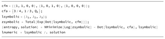
Figure 4. Wolfram Mathematica code for finding the Lagrange parameters (47) using the Legendre transform as a function of $Q_1$.

Our four models are distinguished only by their constraint function average, $⟨F_3⟩=Q_1$, in (39). The details are shown in Table 13.

Table 13. MEP-solution of the kangaroo problem.

	$⟨{\mathit{F}}_{\mathit{j}}⟩$	${\mathit{\lambda }}_{\mathit{j}}$	${\mathit{Q}}_{\mathit{i}}$
$M_{\mathrm{MEP},\mathrm{MaxEnt}}$	$(0.75,0.33,0.25)$	$(1.10,-0.69,0.00)$	$(0.25,0.50,0.08,0.17)$
$M_{\mathrm{MEP},\mathrm{LeastSq}}$	$(0.75,0.33,0.29)$	$(0.79,-1.61,1.16)$	$(0.29,0.46,0.04,0.21)$
$M_{\mathrm{MEP},\mathrm{MaxLog}}$	$(0.75,0.33,0.23)$	$(1.29,-0.31,-0.53)$	$(0.23,0.52,0.11,0.14)$
$M_{\mathrm{MEP},\mathrm{MaxSqrt}}$	$(0.75,0.33,0.24)$	$(1.21,-0.46,-0.31)$	$(0.24,0.51,0.10,0.15)$

The constraint function vectors are shown in the second column. The three Lagrange parameters are shown in the third column. From this column one can learn that all three Lagrange parameters ${\lambda }_j$ vary, even when only the value of $⟨F_3⟩$ is varied. Substituting these $\left({\lambda }_1,{\lambda }_2,{\lambda }_3\right)$ in (46), the probability distributions $Q_i$ of the last column are obtained. In our case, these MEP solutions are the same as those obtained by the variational principle methods in table in Table 6, but this need not be so in general. The Lagrange parameters $({\lambda }_1,{\lambda }_2,{\lambda }_3)$ are related to the covariant coordinates $\left({\theta }^1,{\theta }^2,{\theta }^3\right)$ of information geometry in Section 6.

Close inspection of the table in Table 13 reveals that the Lagrange multiplier ${\lambda }_3=0$ for $M_{\mathrm{MEP},\mathrm{MaxEnt}}$ solution. This is an important observation because it signals that the $F_3\left(X=x_i\right)$ constraint function is redundant and, consequently, can be removed. The solution for the joint probabilities $Q_i$ using only $\left(⟨F_1⟩,⟨F_2⟩\right)$ is identical to the one with $\left(⟨F_1⟩,⟨F_2⟩,⟨F_3⟩\right)$. Actually, we knew this already, as this was the basis of the solution in Table 3, but the MEP provides a systematic method for detecting redundancies ([6], p. 369, [8], p. 108).

The Lagrange parameters can be solved algebraically for the $M_{\mathrm{MEP},\mathrm{MaxEnt}}$ and the $M_{\mathrm{MEP},\mathrm{LeastSq}}$ models. Recall that the $M_{\mathrm{VP},\mathrm{MaxEnt}}$ and $M_{\mathrm{VP},\mathrm{LeastSq}}$ models gave exact solutions for the $Q_i$, namely from substituting (8) and (5) in (2). From (46), we see that $Z=1/Q_4$, therefore the value of the partition function is exactly known. Subsequently, the $exp{\lambda }_j$ can be solved algebraically from (46).

Since the $M_{\mathrm{VP},\mathrm{k}}$ and the $M_{\mathrm{MEP},\mathrm{k}}$ model results turn out to be identical, the distinction based on their solution method can now be dropped. For consistency, we keep the redundant $F_3\left(X=x_i\right)$ constraint function in the $M_{\mathrm{MaxEnt}}$ model.

6. Information Geometry

6.1. Coordinate Systems

In Information Geometry (IG), a discrete probability distribution $Q_i$ is represented by a point in a manifoldS. A manifold of dimension n is denoted by $S^n$; in our case $n=4$. The probability distribution is parameterized by two dual coordinate systems, namely a covariant system denoted by superscripts $\left({\theta }^0,{\theta }^1,{\theta }^2,{\theta }^3\right)$ and a contravariant system denoted by subscripts $\left({\eta }_0,{\eta }_1,{\eta }_2,{\eta }_3\right)$. This notation corresponds to the work of Amari [9]. The book by Blower [8] is entirely devoted to IG, and in this section we follow his notation.

The contravariant coordinate system corresponds to the constraint function averages

$$\left({\eta }_0,{\eta }_1,{\eta }_2,{\eta }_3\right)=\left(⟨F_0⟩,⟨F_1⟩,⟨F_2⟩,⟨F_3⟩\right),$$

(48)

whereas the covariant coordinates are the Lagrange multipliers

$$\left({\theta }^0,{\theta }^1,{\theta }^2,{\theta }^3\right)=\left({\lambda }_0,{\lambda }_1,{\lambda }_2,{\lambda }_3\right).$$

(49)

The normalization of the probability distribution is given by

$$⟨F_0⟩={\eta }_0=1.$$

This definition yields for the first covariant coordinate

$${\lambda }_0={\theta }^0=1-logZ,$$

where Z is the partition function (41). For example, the uniform distribution q in the covariant coordinate system is

$$\left({\lambda }_0,{\lambda }_1,{\lambda }_2,{\lambda }_3\right)=\left(1-log4,0,0,0\right),$$

(50)

and in the contravariant coordinate system

$$\left(⟨F_0⟩,⟨F_1⟩,⟨F_2⟩,⟨F_3⟩\right)=\left(1,1/2,1/2,1/4\right).$$

(51)

In IG, the normalization is always implicitly assumed; therefore the coordinates ${\eta }_0$ and ${\theta }^0$ are never shown explicitly. In the remainder of this paper, only three coordinates are used, namely

$$\left(⟨F_1⟩,⟨F_2⟩,⟨F_3⟩\right)=\left({\eta }_1,{\eta }_2,{\eta }_3\right),$$

(52)

and

$$\left({\lambda }_1,{\lambda }_2,{\lambda }_3\right)=\left({\theta }^1,{\theta }^2,{\theta }^3\right).$$

(53)

6.2. Tangent Space

All modeling takes place in a sub-manifold $S^m$, which is tangent to the manifold $S^n$. This is illustrated in Figure 5. In our kangaroo problem $m=3$.

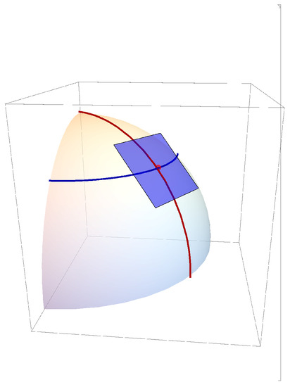
Figure 5. The sub-manifold $S^m$ (blue) is tangent to the manifold $S^n$. The red line is a meridian of longitude and the blue line is a parallel of latitude through the point of tangency.

Perhaps it is tempting to think of a probability distribution Q as a vector in $S^n$, with a coordinate system along the axes as in Figure 6. However, this notion is conceptually wrong because the probability distribution is normalized by

$$Q_1+Q_2+Q_3+Q_4=1,$$

(54)

and not as

$$\sqrt{Q_1^2+Q_2^2+Q_3^2+Q_4^2}=1.$$

(55)

We will return to the issue of normalization in Section 6.6.

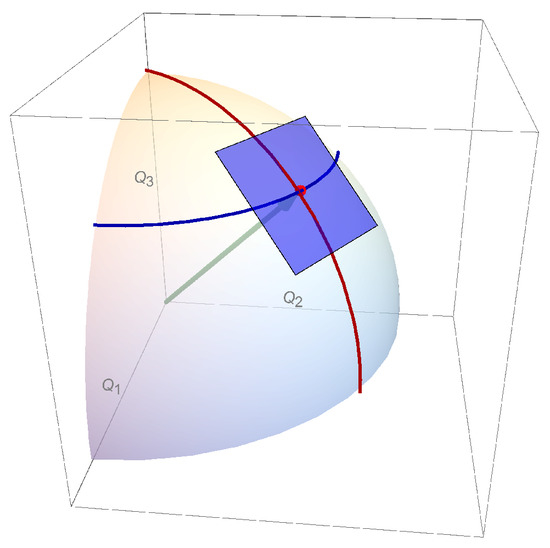
Figure 6. Incorrect view of the probability distribution as a vector (green) to the point of tangency in $S^n$, with a coordinate system along the axes.

The manifold has no familiar extrinsic set of coordinate axes by which all points can be referenced. All we have is this austere representation of points mapped to a coordinate system ([8], p.46). The tangent space is spanned by a set of m basis vectors. The natural basis vectors of the tangent space are

$${\mathbf{e}}_r=F_r\left(X=x_i\right)-⟨F_r⟩,$$

(56)

where we recognize the constraint function vector $F_r\left(X=x_i\right)$ and the corresponding constraint function average $⟨F_r⟩$. Notice that the constraint function average $⟨F_r⟩$ is subtracted from every element of the constraint function vector $F_r\left(X=x_i\right)$. For the least squares model solution $M_{\mathrm{LeastSq}}$, the basis vectors are

$$\left({\mathbf{e}}_1,{\mathbf{e}}_2,{\mathbf{e}}_3\right)=\left(\begin{array}{c}1/4\\ 1/4\\ -3/4\\ -3/4\end{array},\begin{array}{c}2/3\\ -1/3\\ 2/3\\ -1/3\end{array},\begin{array}{c}17/24\\ -7/24\\ -7/24\\ -7/24\end{array}\right),$$

(57)

where we have used (36) and (39), and substituted the $Q_i$ using (5).

These basis vectors are not orthogonal. The angle $\varphi$ between two vectors $\mathbf{v}$ and $\mathbf{w}$ is given by

$$cos\left(\varphi \right)=\frac{\mathbf{v}·\mathbf{w}}{∥\mathbf{v}∥∥\mathbf{w}∥}.$$

(58)

This gives for the angles in degrees between ${\mathbf{e}}_1$ and ${\mathbf{e}}_2$, ${\mathbf{e}}_1$ and ${\mathbf{e}}_3$, and ${\mathbf{e}}_2$ and ${\mathbf{e}}_3$: ${98.1}^{\circ }$, ${56.1}^{\circ }$, and ${59.0}^{\circ },$ respectively. The basis vectors are also not normalized; their lengths are defined as $∥{\mathbf{e}}_r∥$ and found to be $1.12$, $1.05$, and $0.87$, respectively. However, the ${\mathbf{e}}_r$ of (57) are perpendicular to the probability distribution (6) from the model $M_{\mathrm{VP},\mathrm{LeastSq}}$

$$Q_i=(7/24,11/24,1/24,5/24);$$

(59)

all mutual angles $\varphi$ are ${90.0}^{\circ }$.

Since the basis vectors ${\mathbf{e}}_r$ do not form an orthogonal coordinate system, for an arbitrary vector there are two possible projections. Covariant coordinates are obtained by a projection parallel to the basis vectors, while contravariant coordinates are obtained by a perpendicular projection onto the basis vectors.

6.3. Metric Tensor

Each probability distribution p in the manifold $S^n$ has an associated metric tensor $\mathbf{G}\left(p\right)$. The metric tensor is an additional structure that allows the definition of distances and angles in the manifold.

The metric tensor is a symmetric matrix, and it comes in covariant and contravariant forms which are each other’s matrix inverse. The contravariant metric tensor turns out to be the same as the variance-covariance matrix ([8], p. 50). In our notation the covariant form is $g^{rc}$, and the contravariant form is $g_{rc}$, where the superscripts and subscripts r and c refer to the matrix row and column index.

The elements of the contravariant metric tensor are defined as inner products

$$\begin{array}{cc}\hfill g_{rc}& =⟨\left(F_r\left(X=x_i\right)-⟨F_r⟩\right),\left(F_c\left(X=x_i\right)-⟨F_c⟩\right)⟩\hfill \\ \hfill & =\sum _{i=1}^n\left(F_r\left(X=x_i\right)-⟨F_r⟩\right)\left(F_c\left(X=x_i\right)-⟨F_c⟩\right)Q_i\hfill \\ \hfill & =\sum _{i=1}^n{F}_r\left(X=x_i\right)F_c\left(X=x_i\right)Q_i-⟨F_r⟩⟨F_c⟩.\hfill \end{array}$$

(60)

The sum is over all state space cells, whereas the r and c are fixed. Notice that this is the same computation as (22) for the covariance between two vectors.

In the locally flat tangent space $S^m$, the two coordinate systems are non-orthogonal, and the metric tensor forms the local transformation between the two coordinate systems,

$$\frac{\partial ⟨F_c⟩}{\partial {\lambda }_r}=\frac{\partial {\eta }_c}{\partial {\theta }^r}=g_{rc},$$

(61)

and its inverse

$$\frac{\partial {\lambda }_r}{\partial ⟨F_c⟩}=\frac{\partial {\theta }^r}{\partial {\eta }_c}=g^{rc}.$$

(62)

In Blower’s notation the contravariant $⟨F_j⟩$ and covariant ${\lambda }_j$ vector indices do not follow the common Einstein convention.

The metric tensor can be computed by

$$g_{rc}=\frac{{\partial }^{2}logZ}{\partial {\lambda }_r\partial {\lambda }_c},$$

(63)

with Z the partition function (43)

$$Z\left(\lambda \right)=e^{\left({\lambda }_1+{\lambda }_2+{\lambda }_3\right)}+e^{{\lambda }_1}+e^{{\lambda }_2}+1.$$

(64)

The contravariant metric tensor for our kangaroo problem is most easily expressed in the covariant coordinates $\left({\lambda }_1,{\lambda }_2,{\lambda }_3\right)$

$$\mathbf{G}\left(\lambda \right)=\frac{1}{Z^2}\left(\begin{array}{ccc}{e}^{{\lambda }_1}\left(e^{{\lambda }_2}+1\right)\left(e^{{\lambda }_2+{\lambda }_3}+1\right)& e^{{\lambda }_1+{\lambda }_2}\left(e^{{\lambda }_3}-1\right)& e^{{\lambda }_1+{\lambda }_2+{\lambda }_3}\left(e^{{\lambda }_2}+1\right)\\ e^{{\lambda }_1+{\lambda }_2}\left(e^{{\lambda }_3}-1\right)& e^{{\lambda }_2}\left(e^{{\lambda }_1}+1\right)\left(e^{{\lambda }_1+{\lambda }_3}+1\right)& e^{{\lambda }_1+{\lambda }_2+{\lambda }_3}\left(e^{{\lambda }_1}+1\right)\\ e^{{\lambda }_1+{\lambda }_2+{\lambda }_3}\left(e^{{\lambda }_2}+1\right)& e^{{\lambda }_1+{\lambda }_2+{\lambda }_3}\left(e^{{\lambda }_1}+1\right)& e^{{\lambda }_1+{\lambda }_2+{\lambda }_3}\left(e^{{\lambda }_1}+e^{{\lambda }_2}+1\right)\end{array}\right).$$

(65)

The Wolfram Mathematica [5] code which yields this symbolic expression is surprisingly compact, as shown in Figure 7. This short piece of code demonstrates the indispensability of a good symbolic tool when doing IG.

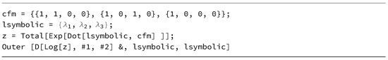
Figure 7. Wolfram Mathematica code for calculating the metric tensor (65).

Substituting the appropriate Lagrange parameters from Table 13, the metric tensor for the least squares model solution $M_{\mathrm{LeastSq}}$ is

$${\mathbf{G}}_{\mathrm{LeastSq}}=\left(\begin{array}{ccc}3/16& 1/24& 7/96\\ 1/24& 2/9& 7/36\\ 7/96& 7/36& 119/576\end{array}\right),$$

(66)

and for the maximum entropy model $M_{\mathrm{MaxEnt}}$, we obtain

$${\mathbf{G}}_{\mathrm{MaxEnt}}=\left(\begin{array}{ccc}3/16& 0& 1/16\\ 0& 2/9& 1/6\\ 1/16& 1/6& 3/16\end{array}\right).$$

(67)

Here we can see that the upper-left $2\times 2$ sub-matrices are identical to the variance-covariance matrix of (24). The extension to the $3\times 3$ matrices is due to the added interactions $F_3\left(X=x_i\right)$.

6.4. Kullback–Leibler Divergence

The Kullback–Leibler divergence allows for the determination of the differences in information content between two probability distributions. The Kullback–Leibler divergence between two discrete probability distributions p and q is defined as

$$KL\left(p\Vert q\right)=\sum _{i=1}^n{p}_{i}log\left(\frac{p_i}{q_i}\right).$$

(68)

The divergence is not a distance because the expression is not symmetric in p and q. A common way to refer to Kullback–Leibler divergence (KL) is as the relative entropy of p with respect to q or the information gained from p over q.

For example, with $p=(0,0,1,0)$ and $q=(1/4,1/4,1/4,1/4)$ we have

$$\begin{array}{cc}\hfill KL\left(p\Vert q\right)& =0log\left(\frac{0}{1/4}\right)+0log\left(\frac{0}{1/4}\right)+1log\left(\frac{1}{1/4}\right)+0log\left(\frac{0}{1/4}\right)\hfill \\ \hfill & =log\left(4\right),\hfill \end{array}$$

(69)

where we have used the limit expression (31) again. However, when we interchange p and q we obtain

$$\begin{array}{cc}\hfill KL\left(q\Vert p\right)& =1/4log\left(\frac{1/4}{0}\right)+1/4log\left(\frac{1/4}{0}\right)+1/4log\left(\frac{1/4}{1}\right)+1/4log\left(\frac{1/4}{0}\right)\hfill \\ \hfill & =\infty .\hfill \end{array}$$

(70)

Therefore, figuratively speaking, we have gained a finite amount of information when learning that we are certain, but we have lost an “infinite” amount when we lose our certainty. Learning and forgetting are asymmetric.

Therefore, the notion of the KL-divergence as a distance measure between distinct probability distributions is flawed. Rewriting (68) we obtain

$$\begin{array}{cc}\hfill KL\left(p\Vert q\right)& =\sum _{i=1}^n{p}_{i}log\left(\frac{p_i}{q_i}\right)\hfill \\ \hfill & =\sum _{i=1}^n{p}_{i}log{p}_i-\sum _{i=1}^n{p}_{i}log{q}_i\hfill \\ \hfill & =-{⟨logq⟩}_p-H\left(p\right)\hfill \end{array}$$

(71)

where $H\left(p\right)$ is the entropy of p. The first term on the right is the expectation of $logq$ with respect to p. When $q\ne p$, $KL\left(p\Vert q\right)$ and $-{⟨logq⟩}_p$ are strictly positive quantities.

The KL-divergence can be expressed in bits when (68) is multiplied by ${log}_{2}e\approx 1.44$. Table 14 shows the values for our four models. As expected, the table is not symmetric.

Table 14. The Kullback–Leibler divergence $KL\left(p\Vert q\right)$ (bits) between the models $M_k$, where p and q are the models in the rows and columns, respectively.

	${\mathit{M}}_{\mathbf{MaxEnt}}$	${\mathit{M}}_{\mathbf{LeastSq}}$	${\mathit{M}}_{\mathbf{MaxLog}}$	${\mathit{M}}_{\mathbf{MaxSqrt}}$
$M_{\mathrm{MaxEnt}}$	0	$0.0368$	$0.0085$	$0.0030$
$M_{\mathrm{LeastSq}}$	$0.0327$	0	$0.0729$	$0.0547$
$M_{\mathrm{MaxLog}}$	$0.0087$	$0.0834$	0	$0.0014$
$M_{\mathrm{MaxSqrt}}$	$0.0031$	$0.0623$	$0.0014$	0

When the distributions p and $q=p+dp$ are infinitesimally close, writing

$$q_i=p_i+d{p}_i,$$

(72)

we have

$$\sum _{i=1}^{n}d{p}_i=0.$$

(73)

Expanding the KL-divergence for small $dp$

$$\begin{array}{cc}\hfill KL\left(p\Vert q\right)& =\sum _{i=1}^n{p}_{i}log\left(\frac{p_i}{q_i}\right)\hfill \\ \hfill & =-\sum _{i=1}^n{p}_{i}log\left(\frac{q_i}{p_i}\right)\hfill \\ \hfill & =-\sum _{i=1}^n{p}_{i}log\left(1+\frac{d{p}_i}{p_i}\right)\hfill \\ \hfill & =-\sum _{i=1}^{n}d{p}_i+\sum _{i=1}^n\frac{1}{2}\frac{d{p}_i^2}{p_i}-O\left(d{p}^3\right)\hfill \\ \hfill & \approx \frac{1}{2}\sum _{i=1}^n\frac{d{p}_i^2}{p_i}.\hfill \end{array}$$

(74)

This expansion is a sum of squares, which is symmetric. Therefore, the KL-divergence is commutative for infinitesimal separations between p and q.

This property of the Kullback–Leibler divergence has an analogy in classical mechanics, namely that two infinitesimal rotations of a rigid body along different principal axes are commutative, while finite rotations are not.

6.5. Distances

What is the distance between two discrete probability distributions p and q in the manifold $S^n$? This is at the heart of Information Geometry. For a distance we need a curve connecting the two points. There are many possibilities. What would be the length of such curves? Which one is the shortest? The shortest of all possible curves is called a geodesic. Suppose that s is a curve connecting p and q, then any point t on the curve s is a probability distribution. Therefore, we have a continuum of probability distributions along s in the manifold $S^n$.

For two close-by points p and $q=p+dp$, their distance is a function of the KL-divergence, namely ([8], pp. 77–78)

$$ds=\sqrt{2KL(p\Vert q)}.$$

(75)

The same distance is given by

$$ds=\sqrt{\sum _{r=1}^m\sum _{c=1}^m{g}_{rc}\left(p\right)d{\lambda }_{r}d{\lambda }_c},$$

(76)

where the covariant coordinates $\lambda$ and $\lambda +d\lambda$ of p and q are used, and the metric tensor $g_{rc}\left(p\right)$ is evaluated as in (65). However, there is a subtle difference here, namely the KL-divergence in (75) is computed in the full manifold $S^n$, whereas $ds$ in (76) is computed in the tangent space $S^m$, with $m<n$.

When the two distributions are finitely separated, as is the case for our models $M_k$, the length of the curve $s\left(t\right)$ is the integral from p to q of

$$L\left(s\right)={\int }_p^q\left|s^{\prime }\left(t\right)\right|dt,$$

(77)

where $s\left(t\right)$ is the curve in $S^n$ parameterized by the probability distribution t, and $s^{\prime }\left(t\right)$ is its first derivative. The tangent sub-manifold $S^m\left(t\right)$ follows t along $s\left(t\right)$ from p to q, and the Lagrange parameters $\lambda \left(t\right)$ and the metric tensor $g_{rc}\left(t\right)$ vary with t. However, finding the distance $D=minL\left(s\right)$ is an Euler–Legendre variational problem beyond the scope of this paper [10].

6.6. Angular Distances

The distance between two probability distributions can also be found as the arc length of a great circle on a sphere in $S^n$. This is known as the Bhattacharyya angle.

Substituting (74) in (75) we can write

$$\begin{array}{cc}\hfill {\left(ds\right)}^2& =\sum _{i=1}^n\frac{{\left(d{p}_i\right)}^2}{p_i}\hfill \\ \hfill & =\sum _{r=1}^m\sum _{c=1}^m{g}_{rc}\left(p\right)d{p}_{r}d{p}_c,\hfill \end{array}$$

(78)

with a metric tensor

$$g_{rc}\left(p\right)=\left\{\begin{array}{cc}1/p_r\hfill & \mathrm{for}r=c\hfill \\ 0\hfill & \mathrm{otherwise}.\hfill \end{array}\right.$$

(79)

Using the transformation

$${\psi }_i=\sqrt{p_i}$$

(80)

we define $\psi$ as a point on the positive orthant of the unit sphere with

$$\sum _{i=1}^n{\psi }_i^2=\sum _{i=1}^n{p}_i=1.$$

(81)

This effectively restricts $\psi$ to a sub-manifold of dimension $S^{n-1}$. The geometry is illustrated by Figure 8. In the $\psi$-coordinate system, the infinitesimal distance becomes

$$\begin{array}{cc}\hfill {\left(ds\right)}^2& =\sum _{i=1}^n\frac{{\left(d{p}_i\right)}^2}{p_i}\hfill \\ \hfill & =\sum _{i=1}^n\frac{{\left(2\psi d{\psi }_i\right)}^2}{{\psi }_i^2}\hfill \\ \hfill & =4\sum _{i=1}^n{\left(d{\psi }_i\right)}^2,\hfill \end{array}$$

(82)

or

$$ds=2d\psi .$$

(83)

Notice that in this coordinate system the metric tensor is the Euclidean metric tensor

$$g_{rc}\left(\psi \right)=\left\{\begin{array}{cc}1\hfill & \mathrm{for}r=c\hfill \\ 0\hfill & \mathrm{otherwise}.\hfill \end{array}\right.$$

(84)

With this transformation the probability distributions become points on a hypersphere with a unit radius in $(n-1)$ dimensions. However, it is well known that geodesics on a sphere are great circles. Therefore, the distance can be obtained by the path integral (77) along a great circle connecting the two points. The arc length between two points is the subtended angle $\theta$ between two points ${\psi }_1$ and ${\psi }_2$ on the unit hypersphere

$$\begin{array}{cc}\hfill \theta & =arccos{\psi }_1·{\psi }_2\hfill \\ \hfill & =arccos\sum _{i=1}^n{\psi }_{1,i}{\psi }_{2,i}\hfill \\ \hfill & =arccos\sum _{i=1}^n\sqrt{p_i}\sqrt{q_i}.\hfill \end{array}$$

(85)

This remarkable result is the Bhattacharyya angle between two probability distributions [11]. The distance D between p and q is twice the arc length from (83)

$$\begin{array}{cc}\hfill D(p,q)& =2\theta \hfill \\ \hfill & =2arccos\sum _{i=1}^n\sqrt{p_i}\sqrt{q_i}.\hfill \end{array}$$

(86)

The units of D are radians. The maximum distance of $\pi$ radians is achieved between two orthogonal distributions.

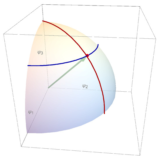
Figure 8. Positive orthant $S^{n-1}$. In the $\psi$-coordinate system, the ${\psi }_i$ are orthonormal coordinates.

With this result we can compute the symmetric distance table for our four Kangaroo models, shown in Table 15; the numerical values are converted from radians to degrees. From this table we see that the largest distance is between the models $M_{\mathrm{LeastSq}}$ and $M_{\mathrm{MaxLog}}$. This observation corresponds with these models having the biggest difference in their correlation coefficients $\rho \left(F_1,F_2\right)$ in Table 11.

Table 15. The distance D (in degree) between the models $M_k$.

${\mathit{M}}_{\mathbf{MaxEnt}}\leftrightarrow {\mathit{M}}_{\mathbf{LeastSq}}$	$12.5$
$M_{\mathrm{MaxEnt}}\leftrightarrow M_{\mathrm{MaxLog}}$	$6.3$
$M_{\mathrm{MaxEnt}}\leftrightarrow M_{\mathrm{MaxSqrt}}$	$3.7$
$M_{\mathrm{LeastSq}}\leftrightarrow M_{\mathrm{MaxLog}}$	$18.8$
$M_{\mathrm{LeastSq}}\leftrightarrow M_{\mathrm{MaxSqrt}}$	$16.3$
$M_{\mathrm{MaxLog}}\leftrightarrow M_{\mathrm{MaxSqrt}}$	$2.5$

Interestingly, when we define lower and upper bounds

$$\begin{array}{cc}\hfill K{L}_{\min }& =min\left(KL\left(p\Vert q\right),KL\left(q\Vert p\right)\right)\hfill \\ \hfill K{L}_{\max }& =max\left(KL\left(p\Vert q\right),KL\left(q\Vert p\right)\right),\hfill \end{array}$$

(87)

all the distances from Table 15 have values

$$\sqrt{2K{L}_{\min }}<D(p,q)<\sqrt{2K{L}_{\max }}.$$

(88)

Although we have no proof, this observation suggests that the two forms of the KL-divergence may act as lower and upper limits for the true distance $D(p,q)$.

6.7. Geodesics

The arc of the great circle connecting the two points can be found as follows [12]. Let $v_1$ and $v_2$ be two points on the $(n-1)$ dimensional hypersphere, then

$$\begin{array}{cc}\hfill w& =v_2-\left(v_2{v}_1\right)v_1\hfill \end{array}$$

(89)

$$\begin{array}{cc}\hfill u& =\frac{1}{∥w∥}w.\hfill \end{array}$$

(90)

Then

$$\alpha \left(\tau \right)=cos\left(\tau \right)v_1+sin\left(\tau \right)u$$

(91)

traces out a great circle through $v_1$ and $v_2$. It starts at $\alpha \left(\tau \right)=v_1$ when $\tau =0$, it reaches $\alpha \left(\tau \right)=v_2$ at $\tau =arccos\left(v_2{v}_1\right)$, and returns to $v_1$ when $\tau =2\pi$. Here we recognize the Bhattacharyya angle again.

When $v_1={\psi }_1$ and $v_2={\psi }_2$ represent two probability distributions, they must remain on the positive orthant of the hypersphere. For $0\le \tau \le arccos\left({\psi }_2{\psi }_1\right)$,

$$t={\alpha }^2\left(\tau \right)$$

(92)

is a probability distribution in $S^n$ on the geodesic connecting ${\psi }_1$ and ${\psi }_2$.

Our under-determined problem is parametrized by a single variable, namely $1/12\le Q_1\le 1/3$ from (3), which implies that there is only one dimension involved. Therefore it seemed reasonable to surmise that varying $Q_1$ traces out probability distributions t along the shortest distance between the various models, but this turned out to be incorrect. The distributions t on the geodesic $s\left(t\right)$ connecting, for example, $M_{\mathrm{LeastSq}}$to $M_{\mathrm{MaxEnt}}$, do not comply with the constraint function average vector (39)

$$\left(⟨F_1⟩,⟨F_2⟩,⟨F_3⟩\right)=\left(3/4,1/3,Q_1\right).$$

(93)

except for the endpoints.

6.8. Distances Revisited

Our knowledge of the geodesic $s\left(t\right)$ allows us to verify (75) with (76). The arc length of the geodesic between p and q is

$$\begin{array}{cc}\hfill s& ={\int }_p^{q}ds\left(t\right)dt\hfill \\ \hfill & ={\int }_p^q\sqrt{\sum _{r=1}^m\sum _{c=1}^m{g}_{rc}\left(t\right)d\lambda {\left(t\right)}_{r}d\lambda {\left(t\right)}_c}dt,\hfill \end{array}$$

(94)

where we have substituted (76). Notice that the metric tensor as well as the covariant coordinates depends on t. This integral can be approximated by a sum of many small steps in t ([8], p.78).

By taking K small segments, the distance s is approximated by

$$s=\sum _{k=0}^{K-1}{\left(\sum _{r=1}^m\sum _{c=1}^m{\left(\lambda \left(t_k\right)-\lambda \left(t_{k+1}\right)\right)}_r{g}_{rc}\left(\lambda \left(t_k\right)\right){\left(\lambda \left(t_k\right)-\lambda \left(t_{k+1}\right)\right)}_c\right)}^{\frac{1}{2}}.$$

(95)

Here $k=0$ corresponds to the probability distribution $t_0=p$ and $k=K$ is the distribution $t_K=q$. The intermediate points $t_k$ are obtained by dividing the arc $0\le \tau \le arccos\left(\sqrt{p}\sqrt{q}\right)$ of the hypersphere into K equal angular segments. The corresponding probability distributions are $t_k={\alpha }^2\left({\tau }_k\right)$, using (92).

For each $t_k$ in (95), the constraint function averages ${\left(⟨F_1⟩,⟨F_2⟩,⟨F_3⟩\right)}_k$ are obtained through the multiplication by the constraint function vectors (36). The corresponding covariant coordinates $\lambda \left(t_k\right)$ are computed by solving the set of equations in (47), as illustrated by Figure 4. Finally, the metric tensor $g_{rc}\left(\lambda \left(t_k\right)\right)$ is obtained through substitution of $\lambda \left(t_k\right)$ in (65). By taking $K=128$ segments and performing the computation of (95) we have confirmed all the numerical values in Table 15. This confirms the equivalence of (75) and (76).

7. Conclusions

The Gull–Skilling kangaroo problem provides a useful setting for illustrating the solution of under-determined problems in probability. The Variational Principle—in conjunction a variational function—effectively creates enough missing information for a complete solution, but not necessarily the minimum amount. In this paper four different Variational Principle solutions are shown, only one of which introduces the minimum amount, when the variational function is the Shannon–Jaynes entropy function.

The Maximum Entropy Principle is an alternative method for solving under-determined problems, which however avoids any implicit introduction of extra information not in the original problem. This information manifests itself in our examples as added correlations in the solutions.

The Kullback–Leibler divergence allows for the determination of the differences in information content between two probability distributions, but it cannot be used as a distance measure. It is symmetrical for infinitesimal separations. We point out an analogy with infinitesimal rigid body rotations.

Through the lens of Information Geometry, the actual geometric distance between two probability distributions along a geodesic path, can also be expressed as twice the Bhattacharyya angle in a hypersphere. In this paper, we illustrate the equivalence of these two geometrical concepts.

We also find that the mutual differences in distance between any two models, are directly reflected in the difference of their correlation coefficients.

Our understanding of the kangaroo problem and its implications has been particularly facilitated by the symbolic programming capabilities of Wolfram Mathematica.

References

- Sivia, D.S.; Skilling, J. Data Analysis, 2nd ed.; Oxford University Press: Oxford, UK, 2006; pp. 111–113. [Google Scholar]
- Gull, S.F.; Skilling, J. Maximum entropy method in image processing. IEE Proc. 1984, 131, 646–659. [Google Scholar] [CrossRef]
- Jaynes, E.T. Monkeys, kangaroos and N. In Maximum Entropy and Bayesian Methods in Applied Statistics; Justice, J. H., Ed.; Cambridge University Press: Calgary, AB, Canada, 1984; pp. 27–58. [Google Scholar]
- Blower, D.J. Information Processing, Volume II, The Maximum Entropy Principle; Third Millennium Inferencing: Pensacola, FL, USA, 2013. [Google Scholar]
- Wolfram Mathematica. Available online: www.wolfram.com (accessed on 7 December 2022).
- Jaynes, E.T. Probability Theory: The Logic of Science; Bretthorst, G.L., Ed.; Cambridge University Press: New York, NY, USA, 2003. [Google Scholar]
- Buck, B; Macaulay, V. A. Maximum Entropy in Action; Oxford University Press: Oxford, UK, 1991. [Google Scholar]
- Blower, D.J. Information Processing, Volume III, Introduction to Information Geometry; Third Millennium Inferencing: Pensacola, FL, USA, 2016. [Google Scholar]
- Amari, S.; Nagaoka, H. Methods of Information Geometry; Originally Published in Japanese by Iwanami Shoten Publishers, Tokyo, Ed.; Translated by D. Harada; Oxford University Press: Oxford, UK, 1993. [Google Scholar]
- Mathews, J.; Walker, R.L. Mathematical Methods of Physics, 2nd ed.; Addison-Wesley Publ.: Menlo Park, CA, USA, 1973; pp. 322–344. [Google Scholar]
- Bhattacharyya, A. On a Measure of Divergence between Two Multinomial Populations. Sankhyā 1946, 7, 401–406. [Google Scholar]
- Mathematics Stack Exchange. Available online: https://math.stackexchange.com/questions/1883904/a-time-parameterization-of-geodesics-on-the-sphere (accessed on 15 September 2022).
Publisher’s Note: MDPI stays neutral with regard to jurisdictional claims in published maps and institutional affiliations. |
© 2022 by the authors. Licensee MDPI, Basel, Switzerland. This article is an open access article distributed under the terms and conditions of the Creative Commons Attribution (CC BY) license (https://creativecommons.org/licenses/by/4.0/).