On Two Measure-Theoretic Aspects of the Full Bayesian Significance Test for Precise Bayesian Hypothesis Testing ^†

Abstract

The Full Bayesian Significance Test (FBST) has been proposed as a convenient method to replace frequentist p-values for testing a precise hypothesis. Although the FBST enjoys various appealing properties, the purpose of this paper is to investigate two aspects of the FBST which are sometimes observed as measure-theoretic inconsistencies of the procedure and have not been discussed rigorously in the literature. First, the FBST uses the posterior density as a reference for judging the Bayesian statistical evidence against a precise hypothesis. However, under absolutely continuous prior distributions, the posterior density is defined only up to Lebesgue null sets which renders the reference criterion arbitrary. Second, the FBST statistical evidence seems to have no valid prior probability. It is shown that the former aspect can be circumvented by fixing a version of the posterior density before using the FBST, and the latter aspect is based on its measure-theoretic premises. An illustrative example demonstrates the two aspects and their solution. Together, the results in this paper show that both of the two aspects which are sometimes observed as measure-theoretic inconsistencies of the FBST are not tenable. The FBST thus provides a measure-theoretically coherent Bayesian alternative for testing a precise hypothesis.

1. Introduction

Statistical hypothesis testing is an important method in a broad range of sciences [1]. However, the recent problems with the validity of research results have been termed a scientific replication crisis [2,3], at the core of which lie some fundamental flaws in the statistical analysis of data [4]. Various papers have discussed the reproducibility of research and often the inadequate use of null hypothesis significance tests (NHST) substantiates a major cause of the replication crisis [5]. This holds in particular in the biomedical and cognitive sciences [6,7], where the p-value is the gold standard for quantifying the evidence against a precise null hypothesis.

Bayesian hypothesis testing has become increasingly popular in the biomedical and cognitive sciences due to the above problems [8,9,10]. It is well known that Bayesian data analysis solves some of the problems of NHST by allowing researchers to make use of optional stopping [11,12] and by simplifying the interpretation of censored data [13]. Together, these aspects are consequence of Bayesian inference being consistent with the likelihood principle [13]. An appealing proposal for a Bayesian test of a precise hypothesis is the Full Bayesian Significance Test (FBST), which has been applied in a wide range of domains [8,14,15,16,17,18]. The FBST advocates the e-value as a Bayesian replacement of the frequentist p-value for quantifying the statistical evidence against a precise hypothesis [19]. The FBST is a fully Bayesian procedure [19], accords with the likelihood principle [15], and enjoys attractive asymptotic properties [20] next to transformation invariance [16]. However, the FBST seems to suffer from two aspects which are studied in detail in this paper. First, the reference criterion in the FBST is only defined up to Lebesgue null sets, which seems to be make the evidential threshold arbitrary. Thus, it seems that the FBST statistical evidence, the e-value, lacks a calibration. Second, the statistical evidence in the FBST seems to have no prior probability, which contradicts common Bayesian reasoning. For other criticisms on the FBST see Ly & Wagenmakers [21] and for a more optimistic perspective Kelter [22]. In this paper it is shown that both aspects can be solved by fixing a version of the posterior distribution for statistical inference, and assigning one of two possible interpretations to the prior probability of the statistical evidence in the FBST. These aspects have not yet been discussed extensively in the literature and present a further justification of the FBST as an attractive replacement of frequentist p-values to remedy the ongoing problems with the replication of scientific results. The plan of the paper is as follows: The next section outlines the theory behind the FBST. After that, the two problematic aspects mentioned above are detailed and illustrated by an example from medical research. The following section elaborates on the problems and provides solutions to them. After that, a conclusion is provided.

2. The Full Bayesian Significance Test

This section outlines the theory behind the FBST. First, the required notation is introduced.

2.1. Notation

In contrast to the frequentist approach, in the Bayesian approach the parameter $\theta \in \mathrm{\Theta }$ is modelled as a random variable, and the data $y\in \mathcal{Y}$ are fixed. Denote by $\mathrm{\Theta }$ the parameter space and $\mathcal{G}$ as the $\sigma$-algebra on $\mathrm{\Theta }$, and let $P_{\vartheta }$ be the prior probability measure on $\mathcal{G}$, leading to the triple $(\mathrm{\Theta },\mathcal{G},P_{\vartheta })$. The observed sample is modelled by the random variable $Y:\mathrm{\Omega }\to \mathcal{Y}$ which takes values in the measurable space $\mathcal{Y}$, where $\mathcal{Y}$ is endowed with a $\sigma$-algebra $\mathcal{B}$. The uncertainty in the data generating mechanism producing a sample $Y\left(\omega \right)=y$ for $\omega \in \mathrm{\Omega }$ is modelled via the assumption of a statistical model $\mathcal{P}:=\{P_{\theta }:\theta \in \mathrm{\Theta }\}$ which is dominated by a $\sigma$-finite measure $\nu$. In practice, $\nu$ often is the Lebesgue measure $\lambda$. The latter requirement guarantees the existence of Radon-Nikodým derivatives $d{P}_{\theta }/d\lambda =f\left(y\right|\theta )$. Let $(\mathrm{\Omega },\mathcal{A},P^{*})$ be the product space defined as $\mathrm{\Omega }:=\mathrm{\Theta }\times \mathcal{Y}$, $\mathcal{A}:=\mathcal{G}\times \mathcal{B}$ and $P^{*}$ the product measure induced by the selection of $P_{\vartheta }$ and $\mathcal{P}$, where $P_{\theta }$ must be a measurable function on $\mathcal{B}$ for every y on $\mathcal{Y}$. Thus, $P_{\vartheta }$ is the marginal distribution of $P^{*}$ with respect to the parameter $\theta$, and the marginal distribution with respect to Y is the prior predictive $P^{\vartheta }\left(B\right):={\int }_{\mathrm{\Theta }}{P}_{\theta }\left(B\right)d{P}_{\vartheta }$ for any $B\in \mathcal{B}$. The parameter, as noted above, is modelled mathematically as a random variable $\vartheta :\mathrm{\Omega }\to \mathrm{\Theta }$. The resulting operational models from a Bayesian point of view are thus given as

(1)

the prior model $(\mathrm{\Theta },\mathcal{G},P_{\vartheta })$

(2)

the statistical model $\mathcal{P}$ on $(\mathcal{Y},\mathcal{B})$, leading to $(\mathcal{Y},\mathcal{B},\{P_{\theta }:\theta \in \mathrm{\Theta }\})$, and

(3)

the posterior model $(\mathrm{\Theta },\mathcal{G},\{P_{\vartheta |Y}:Y\in \mathcal{Y}\})$

The existence of the posterior distribution $P_{\vartheta |Y}$ is guaranteed on Polish spaces [23] and inference about $\theta$ is conducted with respect to the posterior distribution $P_{\vartheta |Y}$ with density $p\left(\theta \right|y):=d{P}_{\vartheta |Y}/d\lambda$, which exists under the assumption that $P_{\vartheta }<<\lambda$ where $<<$ denotes absolute-continuity of $P_{\vartheta }$ with respect to the measure $\lambda$.

2.2. Theory behind the Full Bayesian Significance Test (FBST)

The Full Bayesian Significance Test (FBST) was originally developed by Pereira and Stern [14] as an alternative to frequentist null hypothesis significance tests based on the p-value. It was created under the assumption that a significance test of a sharp hypothesis had to be conducted, where a sharp hypothesis refers to any submanifold of the parameter space of interest [20]. This includes, in particular, precise hypotheses like $H_0:\theta ={\theta }_0$ for ${\theta }_0\in \mathrm{\Theta }$ [15]. The FBST assumes a standard parametric statistical model, where $\theta \in \mathrm{\Theta }\subseteq {\mathbb{R}}^p$ is a (possibly vector-valued) parameter of interest, $f\left(y\right|\theta )$ is the density corresponding to the model distribution $P_{Y|\vartheta }$ and $p\left(\theta \right)$ is the prior density corresponding to the prior distribution $P_{\vartheta }$, where we again assume a dominating measure $\nu$ to guarantee the existence of Radon-Nikodým densities. A hypothesis H makes the statement that the parameter $\theta$ lies in the corresponding null set ${\mathrm{\Theta }}_H$, where for simple (or precise) hypotheses ${\mathrm{\Theta }}_H:=\left\{{\theta }_0\right\}$, where ${\theta }_0$ is the value specified in $H:\theta ={\theta }_0$. The Full Bayesian Significance Test (FBST) then defines two quantities: ev$\left(H\right)$, which is the e-value supporting (or in favour of) the hypothesis H, and $\overline{\mathrm{ev}}\left(H\right)$, the e-value against H, also called the Bayesian evidence value against H [14]. First, the posterior surprise function$s\left(\theta \right)$ and its maximum $s^{*}$ restricted to the null set ${\mathrm{\Theta }}_H$ are introduced:

Definition 1

(Posterior surprise function). The posterior surprise function $s\left(\theta \right)$ for a reference function $r:\mathrm{\Theta }\to (\mathcal{T},\mathcal{C})$ from Θ to a measurable space $(\mathcal{T},\mathcal{C})$ is defined as

$$\begin{array}{c}\hfill s\left(\theta \right):=\frac{p\left(\theta \right|y)}{r\left(\theta \right)}\end{array}$$

(1)

In the definition of the posterior surprise function $s\left(\theta \right)$, the denominator $r\left(\theta \right)$ serves as a reference density, and often the measurable space $(\mathcal{T},\mathcal{C})$ is equal to $({\mathbb{R}}^d,\mathcal{B}\left({\mathbb{R}}^d\right))$. When the improper flat reference function $r\left(\theta \right)=1$ is used, the surprise function becomes the posterior density $p\left(\theta \right|y)$. Otherwise, a weakly informative prior density can be used as a reference function, see Pereira and Stern [16]. Then,

$$\begin{array}{c}\hfill s^{*}:=s\left({\theta }^{*}\right)=\underset{\theta \in {\mathrm{\Theta }}_H}{sup}s\left(\theta \right)\end{array}$$

(2)

is defined as the supremum of the surprise function $s\left(\theta \right)$ over the null hypothesis support. For a precise null hypothesis, $s^{*}$ is simply $s\left({\theta }_0\right)$. Next, the tangential set is introduced:

Definition 2

(Tangential set). The tangential set $\overline{T}\left(\nu \right)$ is defined as

$$\begin{array}{c}\hfill \overline{T}\left(\nu \right):=\mathrm{\Theta }\backslash T\left(\nu \right)\end{array}$$

(3)

where

$$\begin{array}{c}\hfill T\left(\nu \right):=\{\theta \in \mathrm{\Theta }|s\left(\theta \right)\le \nu \}\end{array}$$

(4)

Thus, $T\left(\nu \right)$ includes all parameter values $\theta \in \mathrm{\Theta }$ which attain a surprise function value $s\left(\theta \right)$ smaller or equal to the threshold $\nu$. The tangential set $\overline{T}\left(\nu \right)$ is then the set complement and includes all parameter values $\theta \in \mathrm{\Theta }$ which yield a surprise function value $s\left(\theta \right)$ larger than $\nu$. Fixing $\nu =s^{*}$ yields $\overline{T}\left(s^{*}\right)$, which is called the tangential set to the hypothesis H. This set $\overline{T}\left(s^{*}\right)$ contains the points $\theta$ of the parameter space $\mathrm{\Theta }$ with higher surprise (or corroboration relative to the reference function $r\left(\theta \right)$) than the point ${\theta }_0$ in the null set ${\mathrm{\Theta }}_H$. Then, the cumulative surprise function is introduced which is required to compute the e-value in the final step:

Definition 3

(Cumulative surprise function). The map $W:\mathrm{\Theta }\to [0,1]$ given by

$$\begin{array}{c}\hfill W\left(\nu \right):={\int }_{T\left(\nu \right)}p\left(\theta \right|y)d\theta \end{array}$$

(5)

is called the complementary cumulative surprise function, and

$$\begin{array}{c}\hfill \overline{W}\left(\nu \right):=1-W\left(\nu \right)\end{array}$$

(6)

is called the cumulative surprise function.

Thus, the complementary cumulative surprise function $W\left(\nu \right)$ is the integral of the posterior density $p\left(\theta \right|y)$ over the set $T\left(\nu \right)$, and the cumulative surprise function $\overline{W}\left(\nu \right)$ is simply the integral of the posterior density over the tangential set $\overline{T}\left(\nu \right)$. The final step towards the e-value is to integrate the posterior density $p\left(\theta \right|y)$ over this set:

Definition 4

(e-value). The e-value against a sharp null hypothesis $H_0:\theta ={\theta }_0$ is defined as

$$\begin{array}{c}\hfill \overline{ev}\left(H_0\right):=\overline{W}\left(s^{*}\right)\end{array}$$

(7)

and can be interpreted as the Bayesian evidence against $H_0$.

Clearly, $\overline{\mathrm{ev}}\left(H_0\right):=\overline{W}\left(s^{*}\right)$ is the integral of the density $p\left(\theta \right|y)$ over the tangential set $T\left(s^{*}\right)$, which can be interpreted as the integral of the posterior density $p\left(\theta \right|y)$ over all parameter values $\theta$ which fulfill the condition $s\left(\theta \right)\ge s^{*}$. The e-value ev$\left(H_0\right)$ supporting H is obtained as ev$\left(H\right):=1-\overline{\mathrm{ev}}\left(H_0\right)$ under $r\left(\theta \right):=1$. Large values of $\overline{\mathrm{ev}}\left(H_0\right)$ thus indicate that the hypothesis H traverses low-density regions (or equivalently, that the alternative hypothesis traverses high-density regions) so that the evidence against $H_0$ is large. For $r\left(\theta \right)\ne 1$ the argument is identical as $H_0$ traverses low posterior-surprise regions then.

For theoretical properties of the FBST and the e-value see Pereira and Stern [16] and Kelter [18]. The FBST then uses ev$\left(H\right)$ to reject H if ev$\left(H\right)$ is sufficiently small (or when $\overline{\mathrm{ev}}\left(H\right)$ is large) [14,15].

3. On Two Aspects of the FBST

Now, this section demonstrates the two aspects briefly mentioned in the introduction based on an illustrative example.

3.1. The Reference Criterion

To illustrate the first problem, data of Rosenman et al. [24] of the Western Collaborative Group Study about coronary heart disease is used.

Example 1

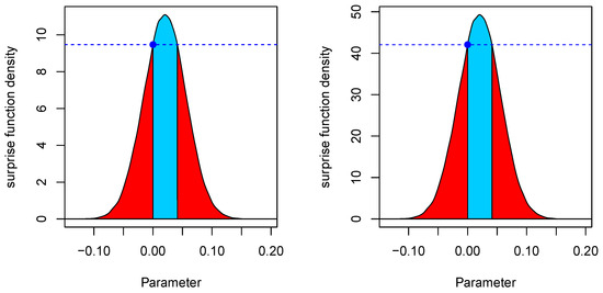
(Coronary heart disease data). The Western Collaborative Group Study began in 1960 with 3524 male volunteers who were 39 to 59 years old and free of heart disease as determined by electrocardiogram. After the initial screening, the study population dropped to 3154 because of various exclusions. Multiple endpoints were studied and average follow-up continued for $8.5$ years with repeat examinations. As an illustrative example, suppose interest lies in testing for differences in systolic blood pressure between light smokers and heavy smokers. Thus, we test the hypothesis $H_0:\delta =0$ against the alternative $H_1:\delta \ne 0$ where we classify participants with more than 5 cigarettes per day as heavy smokers. A Bayesian two-sample t-test using the model of Rouder et al. [25] is conducted, and the left plot in Figure 1 shows the results of the FBST using a flat reference function $r\left(\delta \right):=1$. The model is parameterized in the effect size δ of Cohen [26], and the e-value $\overline{ev}\left(H_0\right)$ is given as $\overline{ev}\left(H_0\right)=0.4362$, which equals the posterior probability mass visualized as the blue area in the left plot of Figure 1. Thus, 43.62% of the posterior probability indicate evidence against the null hypothesis, and the situation is inconclusive. The right plot in Figure 1 shows the result of the FBST when replacing the flat reference function $r\left(\delta \right):=1$ with a Cauchy $C(0,\sqrt{2})$ density (note the different scaling on the y-axis), which is also used as the prior on δ in the two-sample t-test. In this case, the e-value $\overline{ev}\left(H_0\right)=0.4367$ indicates a similarly inconclusive situation and changes the result barely.

Figure 1. Results of the Full Bayesian Significance Test using a flat reference function (left) and a $C(0,\sqrt{2})$ Cauchy density as reference function (right) for testing the hypothesis of no difference $H_0:\delta =0$ in terms of systolic blood pressure between smokers and non-smokers.

Now, the above example shows that calculation of the e-value is straightforward and universally applicable. However, the parameter space $\mathrm{\Theta }$ is continuous in the example (the effect size $\delta \in \mathbb{R}$ is a continuous quantity) and any usual prior distribution $P_{\vartheta }$ assigned to $\theta$ is absolutely continuous with respect to the Lebesgue measure $\lambda$. It is well-known that the posterior distribution $P_{\vartheta |Y}$ is absolutely continuous with respect to the prior distribution [27], and thus any $P_{\vartheta }$-null-set $N\subset \mathrm{\Theta }$ with $P_{\vartheta }\left(N\right)=0$ is also a $P_{\vartheta |Y}$-null-set with $P_{\vartheta |Y}\left(N\right)=0$. Problematically, the set ${\mathrm{\Theta }}_0:=\left\{{\delta }_0\right\}=\left\{0\right\}$ which is used in the precise null hypothesis $H_0:\delta =0$ is a $P_{\vartheta }$-null-set under both the improper flat and Cauchy prior, as both of these are absolutely continuous with respect to the Lebesgue measure $\lambda$, and submanifolds are Lebesgue-null-sets [28]. Thus, $\lambda (\left\{{\delta }_0\right\}=\lambda \left(\left\{0\right\}\right)=0$ implies $P_{\vartheta }\left(\left\{0\right\}\right)=0$ due to $P_{\vartheta }<<\lambda$, which implies in turn that the posterior probability $P_{\vartheta |Y}\left(\left\{0\right\}\right)$ of the value ${\delta }_0=0$ is a $P_{\vartheta |Y}$-null-set due to $P_{\vartheta |Y}<<P_{\vartheta }$. As a consequence, the value of the posterior density $p\left(0\right|y)=9.4693$ which is shown as the blue point in the left plot of Figure 1 could be chosen arbitrarily. Problematically, this value is used as the reference criterion in the calculation of the e-value $\overline{\mathrm{ev}}\left(H_0\right)$ in the computation of the tangential set $\overline{T}\left(\nu \right)$. Thus, one could assign $p\left(0\right|y)$ an entirely different value, say, $c\in \mathbb{R}$, and obtain a different e-value $\overline{\mathrm{ev}}\left(H_0\right)$ than the one calculated from the value $p\left(0\right|y)=9.4693$. This seems to render the calculation of the statistical evidence $\overline{\mathrm{ev}}\left(H_0\right)$ in the FBST arbitrary, questioning the use of the procedure.

3.2. Prior Probability of the e-Value

The second issue with the FBST may be phrased as the e-value having no valid prior probability. In fact, the e-value in Equation (7) is based on the cumulative surprise function $W\left(s^{*}\right)$, which itself depends on the tangential set $T\left(s^{*}\right)$ and the posterior density $p\left(\theta \right|y)$. Before data $y\in \mathcal{Y}$ are observed, the posterior $P_{\vartheta |Y}$ has not been realized as $P_{\vartheta |Y=y}$ and thus there exists no prior probability $P_{\vartheta }$ which is associated with the e-value. Even the tangential set $\overline{T}\left(s^{*}\right):=\{\theta \in \mathrm{\Theta }|s\left(\theta \right)>s^{*}\}$ which is a subset of $\mathrm{\Theta }$ seems to have no prior probability, because it depends on the surprise function $s\left(\theta \right)$ which itself depends on the posterior density $p\left(\theta \right|y)$, compare Equation (1). Thus, the statistical evidence in the FBST seems to escape the natural Bayesian transition from prior to posterior probability.

4. Solutions to the Two Aspects

4.1. The Reference Criterion

If the above criticism that the reference criterion in the FBST is arbitrary would hold, the procedure would be of little use in practice. However, the solution to the problem is given by fixing a specific version of the posterior distribution and performing all calculations conditional on fixing such a version. It is well known that probability distributions (which are probability measures corresponding to a random variable) are defined up to Lebesgue-null-sets (when they are dominated by the Lebesgue measure). The values on null-sets do not influence these probability measures and therefore they are identified with each other whenever they only differ on Lebesgue-null-sets [28]. Technically, this corresponds to the shift from the vector space ${\mathcal{L}}^p$

$$\begin{array}{c}\hfill {\mathcal{L}}^p(\mathrm{\Omega },\mathcal{A},\mu ):=\left\{f:\mathrm{\Omega }\to \mathbb{K}|\mathrm{f}\mathrm{is}\mathrm{measurable},{\int }_{\mathrm{\Omega }}{\left|f\left(x\right)\right|}^{p}d\mu \left(x\right)<\infty \right\}\end{array}$$

(8)

on a probability space $(\mathrm{\Omega },\mathcal{A},\mu )$, $\mathbb{K}\in \{\mathbb{R},\mathbb{C}\}$ for $0<p<\infty$ to the quotient space $L^p$, see Bauer [28]. The latter space is defined as $L^p:={\mathcal{L}}^p/\mathcal{N}$, where

$$\begin{array}{c}\hfill \mathcal{N}:=\left\{f\in {\mathcal{L}}^p|f=0\mu -\mathrm{almost}-\mathrm{everywhere}\right\}\end{array}$$

(9)

and the elements in $L^p$ are equivalence classes. Thus, two elements $\left[f\right],\left[g\right]\in L^p$ are equal if and only if they differ only on $\mu$-null-sets, that is, $\left[f\right]-\left[g\right]\in \mathcal{N}$. Thus, the arbitrariness of the reference criterion in the FBST exists only unless a specific representant of the equivalence class, in which the posterior density $p\left(\theta \right|y)$ is located, is selected. In the context of Example 1, this implies that a specific version of the posterior density $p\left(\delta \right|y)$ needs to be chosen, which fixes the densities value on ${\delta }_0=0$ (and the other values $\delta \in \mathrm{\Theta }$). Thus, setting $p\left({\delta }_0\right|y):=p\left(0\right|y):=9.4693$ explicitly by definition fixes one representant of the equivalence class of $P_{\vartheta |Y}$ and bypasses the problem that the reference threshold $p\left({\delta }_0\right|y)$ in the FBST is arbitrary. Whenever the posterior is obtainable as a closed-form solution, that is, follows a well-known probability density ${\tilde{P}}_{\vartheta |Y}$ with Lebesgue-density $\tilde{p}\left(\theta \right|y)$, setting $p\left(\theta \right|y):=\tilde{p}\left(\theta \right|y)$ as the value of this known probability density $\tilde{p}$ for the posterior density p in the FBST by definition solves the first problem. Whenever numerical techniques like Markov-Chain-Monte-Carlo (MCMC) are used to produce the posterior, the resulting posterior distribution $P_{\vartheta |Y}^{MCMC}$ and the posterior density $p^{MCMC}\left(\theta \right|y)$ approximate the true posterior distribution $P_{\vartheta |Y}$ and the posterior Lebesgue-density $p\left(\theta \right|y)$. Thus, setting $p\left(\theta \right|y):=p^{MCMC}\left(\theta \right|y)$ by definition for a fixed numerical technique like MCMC with given random number generator seed fixes a version of the posterior density and renders the reference threshold in the FBST unique. In Example 1 this equals the choice of $p\left({\delta }_0\right|y):=9.4693$ by definition (as MCMC sampling was used), and $p\left(\delta \right|y):=p^{MCMC}\left(\delta \right|y)$ for all $\delta \in \mathbb{R}$. In summary, the above considerations provide the following result:

Theorem 1.

Let $s^{*}:=s\left({\theta }^{*}\right)=\underset{\theta \in {\mathrm{\Theta }}_H}{sup}s\left(\theta \right)$ be the supremum of the surprise function in the Full Bayesian Significance Test, and ${\mathcal{L}}^p$ and $L^p$ the corresponding vector spaces on $(\mathrm{\Theta },\mathcal{G},P_{\vartheta |Y})$ with quotient space $L^p/\mathcal{N}$ for $\mathcal{N}:=\{f\in {\mathcal{L}}^p|f=0\mu -almost-everywhere\}$. Whenever $P_{\vartheta |Y}$ is a known probability distribution ${\tilde{P}}_{\vartheta |Y}$ with Lebesgue-density $\tilde{p}\left(\vartheta \right|Y)$, defining $p\left(\theta \right|y):=\tilde{p}\left(\theta \right|y)$ pointwise for all $\theta \in \mathrm{\Theta }$ renders the e-value $\overline{ev}\left(H_0\right)$ against $H_0:\theta ={\theta }_0$ for ${\theta }_0\in \mathrm{\Theta }$ well-defined and unique for the choice of $p\left(\theta \right|y)$.

Proof. 

See Appendix A. □

Note that when using numerical methods such as MCMC, ergodic theory ensures that $P_{\vartheta |Y}^{MCMC}\to P_{\vartheta |Y}$ in distribution and $p_{\vartheta |Y}^{MCMC}\to p_{\vartheta |Y}$, that is, the MCMC posterior density approximates the posterior Lebesgue-density pointwise with increasing precision for increasing number of MCMC samples [29]. Thus, fixing a version of the posterior, Theorem 1 extends also to situations where numerical techniques such as MCMC are required.

4.2. Prior Probability of the e-Value

The solution to the second problem is more involved and less technical. Conceptually, from the above line of thought it is immediate that under absolutely continuous priors $P_{\vartheta }$ with respect to the Lebesgue measure $\lambda$, the prior probability $P_{\vartheta }\left({\mathrm{\Theta }}_0\right)$ will be zero for any precise null hypothesis $H_0:={\mathrm{\Theta }}_0$ with ${\mathrm{\Theta }}_0:=\left\{{\theta }_0\right\}$ for ${\theta }_0\in \mathrm{\Theta }$. The posterior $P_{\vartheta |Y}$ is absolutely continuous with respect to the prior $P_{\vartheta }$, so $P_{\vartheta |Y}\left({\mathrm{\Theta }}_0\right)=0$. Thus, it is simply not possible to use a natural Bayesian workflow which assigns positive probability mass to a Lebesgue-null-set ${\mathrm{\Theta }}_0$ whenever the statistician uses an absolutely continuous prior distribution $P_{\vartheta }$ with respect to $\lambda$. Traditional Bayesian hypothesis testing and model selection bypasses this inconvenience by introducing an arbitrary mixture prior structure $P_{\vartheta }:=\varrho {\mathbb{1}}_{{\mathrm{\Theta }}_0}+(1-\varrho ){\tilde{P}}_{\vartheta }$ which assigns positive probability mass $\varrho >0$ to the null set ${\mathrm{\Theta }}_0$, and distributes the rest of the probability mass $(1-\varrho )\in [0,1]$ by means of a probability distribution ${\tilde{P}}_{\vartheta }$ on the alternative hypothesis space ${\mathrm{\Theta }}_1=\mathrm{\Theta }\backslash {\mathrm{\Theta }}_0$. Early proposals of such a mixture prior structure include Jeffreys [30] and Haldane [31], see also Robert [29] and Kleijn [23]. Such a prior allows computation of a Bayes factor, and furthermore, the Bayes factor itself also has no prior probability which is naturally associated with it. Importantly, this mixture prior structure imposes a dichotomy between hypothesis testing and parameter estimation, because such a mixture prior structure is reasonable only from a hypothesis testing perspective. Whenever parameter estimation is the goal, the assignment of probability mass $\varrho >0$ to a specific value is highly questionable and often contradicts reasonable a priori beliefs. In these cases, prior beliefs are expressed better through a prior which is absolutely continuous with respect to the Lebesgue measure $\lambda$.

The FBST avoids the introduction of such a mixture structure and thus allows for a unified prior elicitation which is coherent both from a Bayesian hypothesis testing and Bayesian parameter estimation stance. Importantly, the e-value is intended to be a Bayesian replacement of the frequentist p-value which measures the statistical discrepancy between the observed data to an assumed precise hypothesis. Thus, the e-value provides the Bayesian evidence against such a precise hypothesis. From a measure-theoretic point of view, every precise null hypothesis is assumed to be false and the FBST thus aligns with the empirical rationalism of Popper [32]. For the use of testing a precise hypothesis as an approximation of a small interval hypothesis see Berger [33], Rousseau [34], Rao & Lovric [35] as well as Kelter [36]: Often, the approximation of a small interval hypothesis via a precise point null hypothesis will be bad, and thus the e-value does not assign positive probability mass to such a precise null hypothesis. Instead, the FBST quantifies the discrepancy between the observed data and the hypothetical precise null value, while simultaneously implementing I.J. Good’s principle of least surprise [37,38,39]. Note further that the mathematical introduction of positive prior probability $\varrho >0$ to a precise value ${\theta }_0\in \mathrm{\Theta }$ when using a mixture prior does not render such a precise hypothesis $H_0:\theta ={\theta }_0$ more realistic in practice.

Furthermore, next to its measure-theoretic premises, there exists another argument which weakens the criticism that there is no prior probability of the e-value: When a prior distribution $P_{\vartheta }$ is selected and no data $y\in \mathcal{Y}$ has been observed, the posterior distribution can be identified conceptually as the prior distribution. Thus, replacing the posterior density $p\left(\theta \right|y)$ with the $\lambda$-density $p\left(\theta \right)$ of the prior $P_{\vartheta }$ yields $s\left(\theta \right):=\frac{p\left(\theta \right)}{r\left(\theta \right)}$, which implies that the tangential set $\overline{T}\left(\nu \right):=\mathrm{\Theta }\backslash T\left(\nu \right)$ for $T\left(\nu \right):=\{\theta \in \mathrm{\Theta }|s\left(\theta \right)\le \nu \}$ includes those parameter values $\theta \in \mathrm{\Theta }$ for which $p\left(\theta \right)/r\left(\theta \right)>\nu$. Using the fact that $s^{*}=p\left({\theta }_0\right)/r\left({\theta }_0\right)$ for a precise hypothesis $H_0:\theta ={\theta }_0$ then, yields $\overline{T}\left(\nu \right)=\{\theta \in \mathrm{\Theta }|p\left(\theta \right)/r\left(\theta \right)>p\left({\theta }_0\right)/r\left({\theta }_0\right)\}$. Plugging this tangential set into Equation (6) yields the e-value

$$\begin{array}{c}\hfill \overline{\mathrm{ev}}\left(H_0\right):=\overline{W}\left(s^{*}\right)={\int }_{\overline{T}\left(s^{*}\right)}p\left(\theta \right)d\theta \end{array}$$

which is the integral of the prior density $p\left(\theta \right)$ over $\overline{T}\left(s^{*}\right)$. When the reference function $r\left(\theta \right)$ is chosen as a flat improper prior $r\left(\theta \right):=1$, this becomes

$$\begin{array}{c}\hfill \overline{\mathrm{ev}}\left(H_0\right)={\int }_{\{\theta \in \mathrm{\Theta }|p\left(\theta \right)>p\left({\theta }_0\right)\}}p\left(\theta \right)d\theta \end{array}$$

which is the integral of the prior density $p\left(\theta \right)$ over all values which attain higher prior density values than the null value ${\theta }_0$ in $H_0:\theta ={\theta }_0$. Thus, the e-value in such a case quantifies the discrepancy of the precise hypothesis $H_0:\theta ={\theta }_0$ with the prior beliefs $P_{\vartheta }$. The above line of thought provide the following result:

Theorem 2.

Let $r\left(\theta \right):=1$. In case no data $y\in \mathcal{Y}$ has been observed, the e-value quantifies the discrepancy between the precise hypothesis $H_0:={\mathrm{\Theta }}_0$ for ${\mathrm{\Theta }}_0:=\left\{{\theta }_0\right\}$ and ${\theta }_0\in \mathrm{\Theta }$ and the prior distribution $P_{\vartheta }$, that is,

$$\begin{array}{c}\hfill \overline{ev}\left(H_0\right)=P_{\vartheta }\left(\{\theta \in \mathrm{\Theta }|p\left(\theta \right)>p\left({\theta }_0\right)\}\right)\end{array}$$

(10)

Proof. 

See Appendix A. □

Whenever $r\left(\theta \right)\ne 1$, the interpretation is more complicated because such a reference function incorporates a surprise element into the tangential set, but the conclusions remain the same. The e-value then quantifies the discrepancy between the precise hypothesis and the prior surprise.

5. Discussion

The Full Bayesian Significance Test (FBST) has been proposed as a convenient method to replace frequentist p-values for testing a precise hypothesis [14,15,16]. Although the FBST enjoys various appealing properties [8,19,20,40], two aspects of the FBST are sometimes observed as measure-theoretic inconsistencies of the procedure and have not been discussed rigorously in the literature. First, the FBST uses the posterior density as a reference for judging the Bayesian statistical evidence against a precise hypothesis. However, under absolutely continuous prior distributions, the posterior density is defined only up to Lebesgue null sets which renders the reference criterion arbitrary. Second, the FBST statistical evidence seems to have no valid prior probability. In this paper, it was shown that the former problem can be circumvented by fixing a version of the posterior density before using the FBST. Theorem 1 demonstrated that then, the e-value is well-defined and unique after observing the data $y\in \mathcal{Y}$.

The latter aspect is based on the measure-theoretic premises of the FBST. As shown in this paper, the FBST avoids the use of a mixture prior structure which imposes a dichotomy between Bayesian hypothesis testing and parameter estimation. Thus, the FBST is compatible with absolutely continuous priors with respect to the Lebesgue measure $\lambda$ (the Bayes factor, for example, is not). As a consequence, there exists no prior probability of the e-value and a precise hypothesis $H_0:\theta ={\theta }_0$ under an absolutely continuous prior $P_{\vartheta }$. Theorem 2 showed that even then, the e-value has a proper interpretation from a prior perspective: It quantifies the a priori discrepancy of the hypothesis $H_0$ with the prior beliefs which are expressed by $P_{\vartheta }$ whenever the reference function $r\left(\theta \right)$ is flat. When $r\left(\theta \right)\ne 1$, the interpretation is more difficult but the conclusion remains the same.

Together, the results in this paper show that both of the two aspects which are sometimes observed as measure-theoretic inconsistencies of the FBST are not tenable. The FBST thus provides a measure-theoretically coherent Bayesian alternative for testing a precise hypothesis.

References

- Gigerenzer, G. Mindless statistics. J.-Socio-Econ. 2004, 33, 587–606. [Google Scholar] [CrossRef]
- Pashler, H.; Harris, C.R. Is the Replicability Crisis Overblown? Three Arguments Examined. Perspect. Psychol. Sci. 2012, 7, 531–536. [Google Scholar] [CrossRef]
- Baker, M.; Penny, D. Is there a reproducibility crisis? Nature 2016, 533, 452–454. [Google Scholar] [CrossRef] [PubMed] [Green Version]
- McElreath, R.; Smaldino, P.E. Replication, communication, and the population dynamics of scientific discovery. PLoS ONE 2015, 10, 1–16. [Google Scholar] [CrossRef] [PubMed] [Green Version]
- Ioannidis, J.P.A. What Have We (Not) Learnt from Millions of Scientific Papers with p-Values? Am. Stat. 2019, 73, 20–25. [Google Scholar] [CrossRef] [Green Version]
- Button, K.S.; Ioannidis, J.P.; Mokrysz, C.; Nosek, B.A.; Flint, J.; Robinson, E.S.; Munafò, M.R. Power failure: Why small sample size undermines the reliability of neuroscience. Nat. Rev. Neurosci. 2013, 14, 365–376. [Google Scholar] [CrossRef] [PubMed] [Green Version]
- Kelter, R. Bayesian alternatives to null hypothesis significance testing in biomedical research: A non-technical introduction to Bayesian inference with JASP. BMC Med. Res. Methodol. 2020, 20, 1–12. [Google Scholar] [CrossRef]
- Kelter, R. Analysis of Bayesian posterior significance and effect size indices for the two-sample t-test to support reproducible medical research. BMC Med. Res. Methodol. 2020, 20, 1–18. [Google Scholar] [CrossRef] [Green Version]
- Kelter, R. Bayesian survival analysis in STAN for improved measuring of uncertainty in parameter estimates. Meas. Interdiscip. Res. Perspect. 2020, 18, 101–119. [Google Scholar] [CrossRef]
- Wagenmakers, E.J.; Morey, R.D.; Lee, M.D. Bayesian Benefits for the Pragmatic Researcher. Curr. Dir. Psychol. Sci. 2016, 25, 169–176. [Google Scholar] [CrossRef]
- Edwards, W.; Lindman, H.; Savage, L.J. Bayesian statistical inference for psychological research. Psychol. Rev. 1963, 70, 193–242. [Google Scholar] [CrossRef]
- Hendriksen, A.; de Heide, R.; Grünwald, P. Optional Stopping with Bayes Factors: A Categorization and Extension of Folklore Results, with an Application to Invariant Situations. Bayesian Anal. 2020, in press. [Google Scholar] [CrossRef]
- Berger, J.; Wolpert, R.L. The Likelihood Principle; Institute of Mathematical Statistics: Hayward, CA, USA, 1988. [Google Scholar]
- Pereira, C.A.d.B.; Stern, J.M. Evidence and credibility: Full Bayesian significance test for precise hypotheses. Entropy 1999, 1, 99–110. [Google Scholar] [CrossRef]
- Pereira, C.A.d.B.; Stern, J.M.; Wechsler, S. Can a Significance Test be genuinely Bayesian? Bayesian Anal. 2008, 3, 79–100. [Google Scholar] [CrossRef]
- Pereira, C.A.d.B.; Stern, J.M. The e-value: A fully Bayesian significance measure for precise statistical hypotheses and its research program. São Paulo J. Math. Sci. 2020, 1–19. [Google Scholar] [CrossRef]
- Kelter, R. Simulation data for the analysis of Bayesian posterior significance and effect size indices for the two-sample t-test to support reproducible medical research. BMC Res. Notes 2020, 13, 1–3. [Google Scholar] [CrossRef]
- Kelter, R. fbst: An R package for the Full Bayesian Significance Test for testing a sharp null hypothesis against its alternative via the e-value. Behav. Res. Methods 2021, in press. [Google Scholar] [CrossRef]
- Madruga, M.R.; Esteves, L.G.; Wechsler, S. On the Bayesianity of Pereira-Stern tests. Test 2001, 10, 291–299. [Google Scholar] [CrossRef]
- Diniz, M.; Pereira, C.A.B.; Polpo, A.; Stern, J.M.; Wechsler, S. Relationship between Bayesian and frequentist significance indices. Int. J. Uncertain. Quantif. 2012, 2, 161–172. [Google Scholar] [CrossRef]
- Ly, A.; Wagenmakers, E.J. A Critical Evaluation of the FBST ev for Bayesian Hypothesis Testing. Comput. Brain Behav. 2021, 1–8. [Google Scholar] [CrossRef]
- Kelter, R. On the Measure-Theoretic Premises of Bayes Factor and Full Bayesian Significance Tests: A Critical Reevaluation. Comput. Brain Behav. 2021, 1–11. [Google Scholar] [CrossRef]
- Kleijn, B. The Frequentist Theory of Bayesian Statistics; Springer: Amsterdam, The Netherlands, 2020. [Google Scholar]
- Rosenman, R.H.; Brand, R.J.; Jenkins, D.; Friedman, M.; Straus, R.; Wurm, M. Coronary heart disease in Western Collaborative Group Study. Final follow-up experience of 8 1/2 years. JAMA 1975, 233, 872–877. [Google Scholar] [CrossRef]
- Rouder, J.N.; Speckman, P.L.; Sun, D.; Morey, R.D.; Iverson, G. Bayesian t tests for accepting and rejecting the null hypothesis. Psychon. Bull. Rev. 2009, 16, 225–237. [Google Scholar] [CrossRef]
- Cohen, J. Statistical Power Analysis for the Behavioral Sciences, 2nd ed.; Routledge: Hillsdale, NJ, USA, 1988. [Google Scholar]
- Schervish, M.J. Theory of Statistics; Springer Verlag: New York, NY, USA, 1995. [Google Scholar]
- Bauer, H. Measure and Integration Theory; De Gruyter: Berlin, Germany, 2001. [Google Scholar]
- Robert, C.P. The Bayesian Choice, 2nd ed.; Springer New York: Paris, France, 2007. [Google Scholar] [CrossRef]
- Jeffreys, H. Theory of Probability, 1st ed.; The Clarendon Press: Oxford, UK, 1939. [Google Scholar]
- Haldane, J.B.S. A note on inverse probability. Math. Proc. Camb. Philos. Soc. 1932, 28, 55–61. [Google Scholar] [CrossRef]
- Popper, K. The Logic of Scientific Discovery; Routledge: London, UK; New York, NY, USA, 1959. [Google Scholar] [CrossRef]
- Berger, J. Statistical Decision Theory and Bayesian Analysis; Springer: New York, NY, USA, 1985. [Google Scholar]
- Rousseau, J. Approximating Interval hypothesis: P-values and Bayes factors. In Bayesian Statistics; Bernado, J., Berger, J., Dawid, A., Smith, A., Eds.; Oxford University Press: Valencia, Spain, 2007; Volume 8, pp. 417–452. [Google Scholar]
- Rao, C.R.; Lovric, M.M. Testing point null hypothesis of a normal mean and the truth: 21st Century perspective. J. Mod. Appl. Stat. Methods 2016, 15, 2–21. [Google Scholar] [CrossRef]
- Kelter, R. Bayesian and frequentist testing for differences between two groups with parametric and nonparametric two-sample tests. Wires Comput. Stat. 2020, 13, e1523. [Google Scholar] [CrossRef]
- Good, I. Surprise index. In Encyclopedia of Statistical Sciences; Kotz, S., Johnson, N., Reid, C., Eds.; John Wiley & Sons: New York, NY, USA, 1988; Volume 7. [Google Scholar]
- Good, I. C332. Surprise indexes and p-values. J. Stat. Comput. Simul. 1989, 32, 90–92. [Google Scholar] [CrossRef]
- Good, I.J. C420. The existence of sharp null hypotheses. J. Stat. Comput. Simul. 1994, 49, 241–242. [Google Scholar] [CrossRef]
- Stern, J.M. Significance tests, Belief Calculi, and Burden of Proof in legal and Scientific Discourse. Front. Artif. Intell. Its Appl. 2003, 101, 139–147. [Google Scholar]
Publisher’s Note: MDPI stays neutral with regard to jurisdictional claims in published maps and institutional affiliations. |
© 2021 by the author. Licensee MDPI, Basel, Switzerland. This article is an open access article distributed under the terms and conditions of the Creative Commons Attribution (CC BY) license (https://creativecommons.org/licenses/by/4.0/).