Solution of Fraction Navier–Stokes Equation Using Homotopy Analysis Method

Abstract

In the present study, we aimed to derive analytical solutions of the homotopy analysis method (HAM) for the time-fractional Navier–Stokes equations in cylindrical coordinates in the form of a rapidly convergent series. In this work, we explore the time-fractional Navier–Stokes equations by replacing the standard time derivative with the Katugampola fractional derivative, expressed in the Caputo form. The homotopy analysis method is then employed to obtain an analytical solution for this time-fractional problem. The convergence of the proposed method to the solution is demonstrated. To validate the method’s accuracy and effectiveness, two examples of time-fractional Navier–Stokes equations modeling fluid flow in a pipe are presented. A comparison with existing results from previous studies is also provided. This method can be used as an alternative to obtain analytic and approximate solutions of different types of fractional differential equations applied in engineering mathematics.

1. Introduction

Fractional calculus (FC), a prominent branch of applied mathematics, investigates differentiation and integration of arbitrary (non-integer) order. Owing to its established utility across various scientific and engineering disciplines such as physics, electrochemistry, mathematical biology, and fluid dynamics, FC has garnered substantial attention in recent years. Foundational expositions by many authors like Herrmann [1], Kiryakova [2], Miller and Ross [3], Kilbas et al. [4], Podlubny [5], Alqahtani et al. [6], and Zuo et al. [7,8] provide comprehensive insights into its theoretical framework and computational strategies. These contributions elucidate methods for solving differential equations of real (fractional) order and highlight their relevance to a broad spectrum of applications. Consequently, a range of analytical and semi-analytical approaches have been proposed, including the Residual Power Series (RPS) method [9,10,11,12], Modified Simple Equation (MSE) method [13], the Reduced Differential Transform (RDT) method [14,15], and others.

Modern software has achieved considerable progress in solving linear problems and approximating nonlinear ones. While linear problems have been treated effectively, nonlinear problems continue to pose significant challenges. To address these problems, Liao [16,17] introduced a nonlinear analytical method based on the topological property of homotopy, which can be applied flexibly to solve nonlinear problems. This method converts nonlinear problems into linear problems through converging series, and has been modified (see [11]). Homotopy plays an important role in differential topology and can be applied to find roots of nonlinear algebraic equations. These equations are converted into differential problems with initial conditions solved using numerical methods. The homotopy analysis method (HAM) is suitable for nonlinear problems with both small and large parameters, allowing for control over the convergence region and rate of the approximating series. It has proven effective for boundary value problems associated with partial differential equations modeling various physical phenomena, including both linear and nonlinear problems like the heat equation and the Navier–Stokes equation used in fluid mechanics. The homotopy analysis method (HAM) is based on the concept of homotopy, which originates from Poincaré s research. Continuous mappings are created from initial boundary values to the final solution of the studied equations. An auxiliary linear operator is chosen to construct these continuous mappings, and an auxiliary parameter ensures the convergence of the solution series. This method offers great freedom in choosing initial approximations and auxiliary linear factors, allowing complex nonlinear problems to be transformed into infinitely many simpler linear subproblems, as shown by Liao [11]. Fractional calculus, although relatively new compared to other branches of calculus, has ancient roots dating back to the 17th century. Recently, research in this field has grown significantly, demonstrating its ability to model various physical and mechanical phenomena. This involves extending differentiation from the usual case to the fractional case or adopting new equations where fractional-order differentiation or integration is present (see, for example, [18]). The homotopy analysis method has been adapted to solve fractional-order problems of the Riemann–Liouville type. For instance, Zhang et al. [19] solved an integral differential boundary problem of the Riemann–Liouville type, and the authors of [20] solved a time-fractional Fornberg–Whitham equation using Caputo derivatives, comparing the approximate solution with the exact one. Research continued to solve various equations, including the evolutionary Navier–Stokes equation, where the partial derivative with respect to time was replaced with a fractional partial derivative of the Caputo type using cylindrical coordinates (see, for example, [21,22]). For more details on using this method to solve fractional boundary problems, refer to [23]. In our work, we replaced the Caputo derivative in the evolutionary Navier–Stokes equation with the Caputo–Katugampola derivative for time, using cylindrical derivatives for the other variables. The convergence of the solution was demonstrated using the homotopy analysis method in two cases. We compared the results obtained here with previous results to illustrate the method’s effectiveness. For this purpose, we consider the time-fractional Navier–Stokes equation that controls the fluid flow in a pipe field in cylindrical coordinates, which is given by the following:

$$D_t^{\alpha }U\left(r,t\right)={\rho }_0\left({\displaystyle \frac{{\partial }^{2}U}{{\partial r}^2}}+{\displaystyle \frac{1}{r}}{\displaystyle \frac{\partial U}{\partial r}}\right)+P,\left(r,t\right)\in \mathsf{\Omega }\times \left(0,T\right),0<\alpha \le 1,$$

(1)

with the initial condition

$$U\left(r,0\right)=U_0\left(r\right),$$

(2)

where $D_t^{\alpha }={\displaystyle \frac{d^{\alpha }}{d{t}^{\alpha }}}$ denotes the operator of the Caputo fractional derivative of order $\alpha$; $P$ is the pressure; ${\rho }_0$ is the density; $U$ is the velocity; $t$ is the time and $U_0\left(r\right)$ is a function depending on $r$ only.

This work is divided as follows: Section 2 presents the basic concepts and results in fractional calculus used throughout the document. Section 3 introduces the homotopy analysis method applied to solve the proposed problems. Section 4 is dedicated to the existence and uniqueness of the solution for these problems. Section 5 contains the main results related to applying the homotopy analysis method to the mentioned problems, proving convergence with illustrative example graphs. Finally, the conclusion summarizes this research.

2. Key Concepts of Fractional Calculus

In this section, we review the main definitions and properties of fractional calculus theory that are used in this paper. Below, we begin by establishing some fundamental definitions and outcomes.

Consider a finite or infinite interval $(a,b)\subset {\mathbb{R}}^{+}$. Let $\rho \in {\mathbb{R}}^{+},\alpha \in \mathbb{C}\left(\mathfrak{R}\left(\alpha \right)>0\right),$ and $n=\left[\mathfrak{R}\left(\alpha \right)\right]+1.\Gamma \left(.\right)$ denotes the Gamma Euler function. Putting $\delta =x^{1-\rho }{\displaystyle \frac{d}{x}},$ we denote by $L_{\rho }^p\left(a,b\right)$ the weighted Lebesgue space of measurable functions $\mathrm{f}$ on $(a,b)$ such that ${‖f‖}_{L_{\rho }^p\left(a,b\right)}<\infty ,$ where ${‖f‖}_{L_{\rho }^p\left(a,b\right)}={\int }_a^b\left|f\left(x\right)\right|{\displaystyle \frac{dx}{x^{1-\rho }}},$ and the space $A{C}_{\delta }^n\left(\left[a,b\right]\right)$ is defined by the following:

$$A{C}_{\delta }^n\left(\left[a,b\right]\right)=\left\{f:\left[a,b\right]\to \mathbb{C}:{\delta }^{n-1}f\left(x\right)\in AC\left[a,b\right],\delta =x^{1-\rho }{\displaystyle \frac{d}{x}}\right\}.$$

Definition 1

([24]). The Katugampola fractional integrals of order α are defined as follows:

$${\mathcal{I}}_{a^{+}}^{\alpha ;\rho }f\left(t\right)={\displaystyle \frac{1}{\Gamma \left(\alpha \right)}}{\int }_a^t{\left({\displaystyle \frac{t^{\rho }-x^{\rho }}{\rho }}\right)}^{\alpha -1}f\left(x\right){\displaystyle \frac{dx}{x^{1-\alpha }}},a<t<b,$$

(3)

$${\mathcal{I}}_{b^{-}}^{\alpha ;\rho }f\left(t\right)={\displaystyle \frac{1}{\Gamma \left(\alpha \right)}}{\int }_t^b{\left({\displaystyle \frac{{x^{\rho }-t}^{\rho }}{\rho }}\right)}^{\alpha -1}f\left(x\right){\displaystyle \frac{dx}{x^{1-\alpha }}},a<t<b,$$

(4)

Definition 2

([25]). The left-sided and right-sided Katugampola fractional derivatives of order $\alpha$ are defined as outlined below:

$${{}_t{}^{}\mathcal{D}}_{a^{+}}^{\alpha ,\rho }f\left(t\right)={{\left(\delta \right)}^n\mathfrak{I}}_a^{n-\alpha ;\rho }f\left(t\right)={\displaystyle \frac{{\left(\delta \right)}^n}{\Gamma \left(n-\alpha \right)}}{\int }_a^t{\left({\displaystyle \frac{t^{\rho }-x^{\rho }}{\rho }}\right)}^{n-\alpha -1}f\left(x\right){\displaystyle \frac{dx}{x^{1-\rho }}},$$

(5)

$${{}_t{}^{}\mathcal{D}}_{b^{-}}^{\alpha ,\rho }f\left(t\right)={\left(-\delta \right)}^n{\mathfrak{I}}_b^{n-\alpha ;\rho }f\left(t\right)={\displaystyle \frac{{\left(-\delta \right)}^n}{\Gamma \left(n-\alpha \right)}}{\int }_t^b{\left({\displaystyle \frac{x^{\rho }-t^{\rho }}{\rho }}\right)}^{n-\alpha -1}f\left(x\right){\displaystyle \frac{dx}{x^{1-\rho }}},$$

(6)

The following is the definition of the Caputo-type modification of left- and right-sided Katugampola fractional derivatives:

Definition 3

([25]). The following defines the left- and right-sided Caputo–Katugampola fractional derivatives of the order $\alpha$:

$${{}_t{}^{CK}\mathcal{D}}_{a^{+}}^{\alpha ,\rho }f\left(t\right)={\displaystyle \frac{1}{\Gamma \left(n-\alpha -1\right)}}{\int }_a^t{\left({\displaystyle \frac{t^{\rho }-x^{\rho }}{\rho }}\right)}^{n-\alpha -1}{\left(\delta \right)}^{n}f\left(x\right){\displaystyle \frac{dx}{x^{1-\rho }}},$$

(7)

$${{}_t{}^{CK}\mathcal{D}}_{b^{-}}^{\alpha ,\rho }f\left(t\right)={\displaystyle \frac{1}{\Gamma \left(n-\alpha -1\right)}}{\int }_t^b{\left({\displaystyle \frac{x^{\rho }-t^{\rho }}{\rho }}\right)}^{n-\alpha -1}{\left(-\delta \right)}^{n}f\left(x\right){\displaystyle \frac{dx}{x^{1-\rho }}},$$

(8)

Remark 1

([25]). In particular, for $\rho =1or\rho \to 0^{+}$, the fractional derivatives of Hadamard and Riemann–Liouville are acquired, respectively.

Theorem 1

([26]). Let$f\in C_{\delta }^n\left(a,b\right),\alpha >\beta >0and\rho >0witha<t<b$, then

$${{}_t{}^{}\mathcal{D}}_{a^{+}}^{\alpha ,\rho }{\mathcal{I}}_{a+}^{\alpha ,\rho }f\left(t\right)=f\left(t\right),$$

(9)

Theorem 2

([27]). Let $f\in C_{\delta }^n\left(a,b\right).Then,$

$${\mathcal{I}}_{a+}^{\alpha ,\rho }{{}_t{}^K\mathcal{D}}_a^{\alpha ,\rho }f\left(x,t\right)=f\left(t\right)-\sum _{k=0}^{n-1}{\displaystyle \frac{f^{\left[k\right],\rho }\left(a\right)}{k!}}{\left({\displaystyle \frac{t^{\rho }-x^{\rho }}{\rho }}\right)}^k.$$

(10)

Definition 4

([22]). Let $\alpha ,m>0$. The power series is the representation of the one-parameter Mittag–Leffler function, defined as follows:

$$E_{\alpha ,m}\left(t\right)=\sum _{m=0}^{\infty }{\displaystyle \frac{t^m}{\Gamma \left(m\alpha +1\right)}}.$$

(11)

3. Homotopy Analysis Method

3.1. Illustration

The HAM proposed by Liao [11] aims to obtain an exact solution for both linear and nonlinear differential equations based on an initial estimate. In this section, we discuss the basic ideas of this method. We examine the general form of the following nonlinear differential equation:

$$\mathcal{N}\left(U\left(x,t\right)\right)=0,$$

(12)

where $U$ is an unknown function; x and t are independent variables; and $\mathcal{N}$ is a nonlinear differential operator. Then, we create what is called zero-order deformation equation:

$$\left(1-p\right)\mathcal{D}\left[\psi \left(x,t;p\right)-U_0\left(x,t\right)\right]=phG\left(x,t\right)\mathcal{N}\left[\phi \left(x,t;p\right)\right],$$

(13)

where $p\in [0,1]$ is an embedding parameter; $h\ne 0$ is an auxiliary parameter; $G$ is an auxiliary function; and $\phi \left(x,t;p\right)$ is a function of $x$, $t$ and $p$. Let $U_0$ be an initial approximation of Equation (12), and $\mathcal{D}$ = ${{}_t{}^{CK}\mathcal{D}}_a^{\alpha ,\rho }$ denote an auxiliary linear differential operator with the property, as follows:

$$\mathcal{D}\left[\phi \left(x,t\right)\right]=0,for\phi \left(x,t\right)=0,\phi \left(x,t;p=0\right)=U_0\left(x,t\right),\mathrm{and}\phi \left(x,t;p=1\right)=U\left(x,t\right).$$

From the initial guess $U_0$ to the solution $U\left(x,t\right)$, the solution $\phi \left(x,t;p\right)$ fluctuates depending on the embedding parameter as $p$ increases from 0 to 1.

Develop $\phi \left(x,t;p\right)$ in a Taylor’s series with respect to$\mathrm{p}$, we obtain

$$\phi \left(x,t;p\right)=U_0\left(x,t\right)+{\sum }_{n=1}^{\infty }{U}_n\left(x,t\right)p^n,$$

(14)

where

$$U_n\left(x,t\right)={\displaystyle \frac{1}{n!}}{\displaystyle \frac{{\partial }^n}{\partial p^n}}\phi \left(x,t;p\right){|}_{p=0}.$$

In the following, we assume that the auxiliary parameter, the function $G\left(x,t\right)$, the initial approximation $U_0$, and the auxiliary linear operator $\mathcal{D}$ = ${{}_t{}^{CK}\mathcal{D}}_a^{\alpha ,\rho }$ are carefully chosen so that the series Equation (14) converges at $p=1$. Then, the series Equation (14), at $p$ = 1, becomes

$$U\left(x,t\right)=\phi \left(x,t;p=1\right)=U_n\left(x,t\right)=U_0\left(x,t\right)+\sum _{n=1}^{\infty }{U}_n\left(x,t\right).$$

Differentiating Equation (13) n-times with respect to $p$, then setting $p=0$, and dividing it by $n!$, we obtain the nth-order deformation equation:

$$\mathcal{D}\left[U_n\left(x,t\right)-{{\delta }_{n}U}_{n-1}\left(x,t\right)\right]=hG\left(x,t\right){\mathcal{R}}_n\left(U_{n-1},x,t\right),$$

(15)

with

$$U_n=\left\{U_0,U_1\left(x,t\right),\dots ,U_n\right\}\mathrm{and}$$

$${\mathcal{R}}_n\left(U_{n-1},x,t\right)={\displaystyle \frac{1}{\left(n-1\right)!}}{\displaystyle \frac{{\partial }^{n-1}}{\partial p^{n-1}}}\mathcal{N}\left[\phi \left(x,t;p\right)\right]{|}_{p=0},$$

(16)

where the notation was introduced

$${\delta }_n=\left\{\begin{array}{c}0,n\le 1,\\ 1,n>1.\end{array}\right.$$

(17)

On both sides of Equation (6), we operate the fractional integral operator ${\mathcal{I}}_a^{\alpha ;\rho }$ provided by Equation (3), and we obtain

$$\begin{gathered} U_n\left(x,t\right)={{\delta }_{n}U}_{n-1}\left(x,t\right)-{\delta }_n\sum _{k=0}^{m-1}{\displaystyle \frac{U_{n-1}^{\left[k\right],\frac{t^{\rho }}{\rho }}\left(x,a\right)}{n!}}{\left({\displaystyle \frac{t^{\rho }-a^{\rho }}{\rho }}\right)}^k \\ +hG\left(x,t\right){\mathcal{I}}_a^{\alpha ;\rho }\left[{\mathcal{R}}_n\left(U_{n-1},x,t\right)\right], \\ n\ge 1. \end{gathered}$$

(18)

Therefore, we calculate $U_1\left(x,t\right)$, $U_2\left(x,t\right)$, …, $U_N\left(x,t\right)$ via Equation (18). Hence, the Nth-order approximation of $U\left(x,t\right)$ is given by $U\left(x,t\right)={\sum }_{n=0}^N{U}_n\left(x,t\right),$ and for $N\to \infty$, we obtain an accurate approximation of Equation (12).

Theorem 3

([20]). Since the solution $U\left(x,t\right)=U_0\left(x,t\right)+{\sum }_{n=0}^{\infty }{U}_n\left(x,t\right)$ converges where  $U_n\left(x,t\right)$ is governed by Equation (15) according to Equations (16) and (17), it is natural to be a solution to Equation (12).

Proof. 

Refer to [11]. □

3.2. Existence and Uniqueness

This section shows that a solution to fractional NS Equation (1) with the initial condition (2) is unique using the Banach fixed-point theorem. Let us define a Banach space $C\left(\Omega \times \left[0,T\right]\right)$ first.

$$C(\Omega \times [0,T\left]\right)=:\{U\mid Uiscontinuouson\Omega \times \left[0,T\right],$$

with the norm

$$‖U‖={sup}_{(r,t)\in \Omega \times [0,T]}\left|U\right(r,t\left)\right|.$$

The following theorem deals with the existence and uniqueness of the solution for fractional NS Equation (1) under condition (2).

Theorem 4

([22]). Assume that $f\left(U\left(r,t\right)\right)=P+{\rho }_0\left(\left({\displaystyle \frac{{\partial }^{2}U}{{\partial r}^2}}+{\displaystyle \frac{1}{r}}{\displaystyle \frac{\partial U}{\partial r}}\right)\right)$ uses the Lipschitz constant  $L$ to satisfy the Lipschitz condition if  ${\displaystyle \frac{L}{\Gamma \left(1+\alpha \right)}}{\displaystyle \frac{T^{\rho \alpha }}{{\rho }^{\alpha }}}<1$, and that  $U(r,t)$ is continuous with its first and second partial derivatives continuous on  $\Omega \times [0,T]$. There is unique solution  $U(r,t)$ on  $\Omega \times [0,T]$ for the fractional NS equations described by Equations (1) and (2).

4. Applications of HAM on FNS Equations

The time-fractional Navier–Stokes equation in cylindrical coordinates is solved in this part using the HAM. This approach has the benefit that the auxiliary parameter $h$ can actually be used to regulate and change the convergence region and pace of the solution series [11,27,28].

4.1. First Application

Consider the following time-fractional Navier–Stokes equation in cylindrical coordinates [29,30,31], given by Equation (1), which is as follows:

$${}_t{}^{CK}{\mathcal{D}}_a^{\alpha ,\rho }U\left(r,t\right)={\rho }_0\left({\displaystyle \frac{{\partial }^{2}U}{{\partial r}^2}}+{\displaystyle \frac{1}{r}}{\displaystyle \frac{\partial U}{\partial r}}\right)+P,\left(r,t\right)\in \mathsf{\Omega }\times \left(0,T\right),\rho >0,0<\alpha \le 1,$$

(19)

with the initial condition

$$U\left(r,0\right)=1-r^2,$$

(20)

where $CK\mathrm{i}\mathrm{s}Caputo\text{–}Katugampola,\rho >0$; $P$ is the pressure; ${\rho }_0$ is the density; $U$ is the velocity; t is the time; $U_0\left(r\right)$ is a function depending on $r$ only; $P=-{\displaystyle \frac{1}{{\rho }_1}}{\displaystyle \frac{\partial P}{\partial z}}$ and ${\rho }_0$ represent the kinematics viscosity.

Applying HAM on both sides of Equation (19) and considering the initial condition provided by Equation (20), it is practical to select the first guess as follows:

$$U_0\left(r,0\right)=1-r^2,$$

(21)

and the linear differential operator

$$\mathcal{D}\left[\phi \left(x,t;p\right)\right]={}_t{}^{CK}{\mathcal{D}}_a^{\alpha ,\rho }\left[\phi \left(r,t;p\right)\right],$$

we obtain

$$\mathcal{N}\left[\phi \left(r,t;p\right)\right]={}_t{}^{CK}{\mathcal{D}}_a^{\alpha ,\rho }\left[\phi \left(r,t;p\right)\right]-{\rho }_0\left({\displaystyle \frac{{\partial }^2}{{\partial r}^2}}\phi \left(r,t;p\right)+{\displaystyle \frac{1}{r}}{\displaystyle \frac{\partial }{\partial r}}\phi \left(r,t;p\right)\right)-P\left(1-{\delta }_n\right).$$

(22)

Using Equation (22) and the assumption $G(r,t)=1$, we construct the zero-order deformation equations:

$$\left(1-p\right)\mathcal{D}\left[\phi \left(r,t;p\right)-U_0\left(r,t\right)\right]=ph\mathcal{N}\left[\phi \left(r,t;p\right)\right].$$

(23)

Naturally, if $p=0$ and $p=1$, we obtain $\phi \left(r,t;p=0\right)=U_0\left(r,t\right),$ and $\phi \left(r,t;p=1\right)=U\left(r,t\right),$ correspondingly. Thus, the equation for nth-order deformation is as follows:

$$\mathcal{D}\left[U_n\left(r,t\right)-{{\delta }_{n}U}_{n-1}\left(r,t\right)\right]=h{\mathcal{R}}_n\left(U_{n-1},r,t\right),$$

(24)

subject to the initial condition $U_n\left(r,a\right)=0$, where Equation (17) defines ${\delta }_n$ and

$${\mathcal{R}}_n\left(U_{n-1},r,t\right)={}_t{}^{CK}{\mathcal{D}}_a^{\alpha ,\rho }\left[U_{n-1}\left(r,t\right)\right]-{\rho }_0\left({\displaystyle \frac{{\partial }^2}{{\partial r}^2}}{U}_{n-1}\left(r,t\right)+{\displaystyle \frac{1}{r}}{\displaystyle \frac{\partial }{\partial r}}{U}_{n-1}\left(r,t\right)\right)-P\left(1-{\delta }_n\right).$$

The integral fractional operator ${\mathcal{I}}_a^{\alpha ;\rho }$ is now applied on both sides of Equation (24), giving us

$$\begin{gathered} {\mathcal{I}}_a^{\alpha ;\rho }{}_t{}^{CK}{\mathcal{D}}_a^{\alpha ,\rho }\left[U_n\left(r,t\right)-{{\delta }_{n}U}_{n-1}\left(r,t\right)\right] \\ =h{\mathcal{I}}_a^{\alpha ;\rho }\left[{}_t{}^{CK}{\mathcal{D}}_0^{\alpha ,\rho }{U}_{n-1}\left(r,t\right)\right]-{\rho }_0\left({\displaystyle \frac{{\partial }^2}{{\partial r}^2}}{U}_{n-1}\left(r,t\right)+{\displaystyle \frac{1}{r}}{\displaystyle \frac{\partial }{\partial r}}{U}_{n-1}\left(r,t\right)\right)-P\left(1-{\delta }_n\right), \end{gathered}$$

and applying Theorem 2 to calculate the following result

$$\begin{gathered} U_n\left(r,t\right)-\sum _{k=0}^{m-1}{\displaystyle \frac{U_n^{\left[k\right],\frac{t^{\rho }}{\rho }}\left(r,a\right)}{n!}}{\left({\displaystyle \frac{t^{\rho }-a^{\rho }}{\rho }}\right)}^k-{{\delta }_{n}U}_{n-1}\left(r,t\right)+{\delta }_n\sum _{k=0}^{m-1}{\displaystyle \frac{U_{n-1}^{\left[k\right],\frac{t^{\rho }}{\rho }}\left(r,a\right)}{n!}}{\left({\displaystyle \frac{t^{\rho }-a^{\rho }}{\rho }}\right)}^k \\ =h\left\{U_{n-1}\left(r,t\right)\sum _{k=0}^{m-1}{\displaystyle \frac{U_{n-1}^{\left[k\right],\frac{t^{\rho }}{\rho }}\left(r,a\right)}{n!}}{\left({\displaystyle \frac{t^{\rho }-a^{\rho }}{\rho }}\right)}^k \\ -{\mathcal{I}}_a^{\alpha ;\rho }\left[{\rho }_0\left({\displaystyle \frac{{\partial }^2}{{\partial r}^2}}{U}_{n-1}\left(r,t\right)+{\displaystyle \frac{1}{r}}{\displaystyle \frac{\partial }{\partial r}}{U}_{n-1}\left(r,t\right)\right)+P\left(1-{\delta }_n\right)\right]\right\},n\ge 1. \end{gathered}$$

(25)

For $0<\alpha \le 1$, we have $m=1,$ and the last equation can be rewritten as follows:

$$\begin{gathered} U_n\left(r,t\right)={\left(h+{\delta }_n\right)U}_{n-1}\left(r,t\right)-{\left(h+{\delta }_n\right)U}_{n-1}\left(r,a\right) \\ -h{\mathcal{I}}_a^{\alpha ;\rho }\left[{\rho }_0\left({\displaystyle \frac{{\partial }^2{U}_{n-1}\left(r,t\right)}{{\partial r}^2}}+{\displaystyle \frac{1}{r}}{\displaystyle \frac{\partial U_{n-1}\left(r,t\right)}{\partial r}}\right)+P\left(1-{\delta }_n\right)\right],n\ge 1. \end{gathered}$$

(26)

From the initial guess of Equations (21) and (26), we obtain

$$U_0\left(r,t\right)=1-r^2,$$

$$\begin{gathered} U_1\left(r,t\right)=-h{\mathcal{I}}_a^{\alpha ;\rho }\left[{\rho }_0\left({\displaystyle \frac{{\partial }^2}{{\partial r}^2}}{U}_0\left(r,t\right)+{\displaystyle \frac{1}{r}}{\displaystyle \frac{\partial }{\partial r}}{U}_0\left(r,t\right)\right)+P\right] \\ =-h\left(P-4{\rho }_0\right){\displaystyle \frac{{\left(\frac{t^{\rho }-a^{\rho }}{\rho }\right)}^{\alpha }}{\Gamma \left(\alpha +1\right)}}, \end{gathered}$$

$$\begin{gathered} U_2\left(r,t\right)=\left(1+h\right)U_1\left(r,t\right)-h{\mathcal{I}}_a^{\alpha ;\rho }\left[{\rho }_0\left({\displaystyle \frac{{\partial }^2}{{\partial r}^2}}{U}_1\left(r,t\right)+{\displaystyle \frac{1}{r}}{\displaystyle \frac{\partial }{\partial r}}{U}_1\left(r,t\right)\right)\right] \\ =-\left(1+h\right)h\left(P-4{\rho }_0\right){\displaystyle \frac{{\left(\frac{t^{\rho }-a^{\rho }}{\rho }\right)}^{\alpha }}{\Gamma \left(\alpha +1\right)}}, \end{gathered}$$

$$\begin{gathered} U_3\left(r,t\right)=\left(1+h\right)U_2\left(r,t\right)-h{\mathcal{I}}_a^{\alpha ;\rho }\left[{\rho }_0\left({\displaystyle \frac{{\partial }^2}{{\partial r}^2}}{U}_2\left(r,t\right)+{\displaystyle \frac{1}{r}}{\displaystyle \frac{\partial }{\partial r}}{U}_2\left(r,t\right)\right)\right] \\ =-{\left(1+h\right)}^{2}h\left(P-4{\rho }_0\right){\displaystyle \frac{{\left(\frac{t^{\rho }-a^{\rho }}{\rho }\right)}^{\alpha }}{\Gamma \left(\alpha +1\right)}}, \\ ⋮ \end{gathered}$$

A precise approximation of Equation (19) is provided by the following:

$$\begin{gathered} U\left(r,t\right)=U_0\left(r,t\right)+U_1\left(r,t\right)+U_2\left(r,t\right){+U}_3\left(r,t\right)+\cdots \\ =1-r^2-h\left(P-4{\rho }_0\right){\displaystyle \frac{{\left(\frac{t^{\rho }-a^{\rho }}{\rho }\right)}^{\alpha }}{\Gamma \left(\alpha +1\right)}}\sum _{i=0}^{\infty }{\left(1+h\right)}^i. \end{gathered}$$

(27)

The above series converges for all $h$ in $\left|1+h\right|<1,$ according to geometric series, and we may rewrite it as outlined below:

$$U\left(r,t\right)=1-r^2+{\displaystyle \frac{\left(P-4{\rho }_0\right)}{\Gamma \left(\alpha +1\right)}}{\left({\displaystyle \frac{t^{\rho }-a^{\rho }}{\rho }}\right)}^{\alpha }.$$

(28)

This is an exact solution. Note that there is no relationship between h and the series.

For Equation (28), there are two noteworthy exceptional instances. First, putting $a=0$ and $\rho =1$ into Equation (28), we obtain the following:

$$U\left(r,t\right)=1-r^2+{\displaystyle \frac{\left(P-4{\rho }_0\right)}{\Gamma \left(\alpha +1\right)}}{t}^{\alpha }$$

(29)

Equation (29) provides the same solution as that derived by Oliveira et al. using HAM [21], Momani et al. using ADM [30], Ragab et al. [31] using HAM, and Bairwa et al. [29] using the iterative Laplace transform. Observe that the solution for $P=2$ is t-independent in addition to meeting the initial condition (Figure 1, Figure 2, Figure 3, Figure 4, Figure 5, Figure 6 and Figure 7). We utilize graphics to illustrate the time-fractional derivative solutions to the NS problem in Figure 1, Figure 2, Figure 3, Figure 4, Figure 5, Figure 6 and Figure 7, where the values of $\rho$ and $\alpha$ are varied, while $r$ is set at 0.8. Additionally, we examine the coefficient found in Equation (28) from the angles of $P-4>0$ and $P-4<0$. Specifically, we look at the cases where $P=2$, as shown in Figure 1 and Figure 2, and $P=6$, as shown in Figure 3 and Figure 4. Figure 1 illustrates that the fluid flows in a negative direction when the coefficient $P-4<0$, and that the parameter $\rho$ has an inverse relationship with the fluid flow speed while maintaining $\alpha =1;\alpha =0.95;\alpha =0.65;\alpha =0.35.$ Two views of the fluid flow’s speed are displayed in Figure 2. First, we find that the fluid flow rate exhibits an inverse relationship with the fractional derivative order when $\rho <0.45$. Nevertheless, this connection changes to direct proportionality as the fluid travels through time. Put another way, the fluid flow speed increases in proportion to the increase in the order of the fractional derivative. From an alternative viewpoint, the speed of fluid flow falls in an inverse-proportional manner as the order of the fractional derivative grows when $\rho \ge 1$. This suggests that the fluid flow velocity depends on the parameter $\rho .$ In Figure 3, fluid flow moves in a positive direction when coefficient $P-4>0$. There is an inverse relationship between the fluid flow speed and the parameter $\rho$. The fluid flow speed decreases with increasing $\rho$ value while maintaining the fractional order $\alpha =0.35;0.65;0.95;1.$ The solution (28) at various values of $\alpha$, with $\rho \ge 1$ and the start of the period time at $\rho =0.45$, are shown in Figure 4. It is clear that there is an inverse relationship between the fractional order derivative and the fluid flow speed. Nevertheless, there is a direct association between the fractional order derivative and the fluid flow speed beyond a given interval with $\rho =0.45$. This suggests that the fluid flow’s speed is influenced by the fractional order. Figure 5 and Figure 6 demonstrate that when the coefficient $P-4<0$ or $P-4>0$, we can see that the fluid flow moves in a negative direction. The parameter $\rho$ and the speed of the fluid flow have an inverse correlation. As the value of $\rho$ increases, the speed of the fluid flow decreases while keeping the fractional order $\alpha =1;\alpha =0.95;\alpha =0.65;\alpha =0.35.$

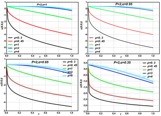
Figure 1. The graphs of Equation (28) displaying different values of parameters $\rho$ with a $=0,P=2,\alpha =1;\alpha =0.95;\alpha =0.65;\alpha =0.35$.

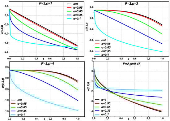
Figure 2. The graphs of Equation (28) displaying different values of parameters $\alpha$ with $a=0;\rho =1;\rho =3;\rho =4;\rho =0.45$.

Figure 3. The graphs of Equation (28) displaying different values of parameters $\rho$ with $a=0;P=6;\alpha =1;\alpha =0.95;\alpha =0.65;\alpha =0.35$.

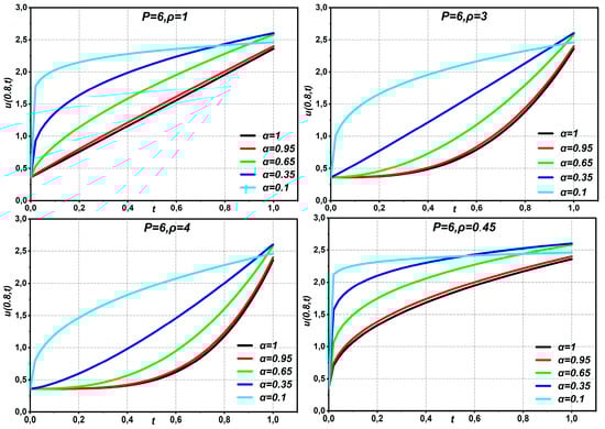
Figure 4. The graphs of Equation (28) displaying different values of parameters $\alpha$ with $a=0;\rho =1;\rho =3;\rho =4;\rho =0.45$.

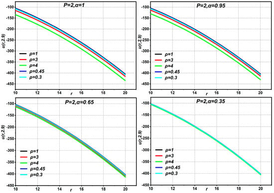
Figure 5. The graphs of Equation (28) displaying different values of parameters $\alpha$ with $a=0;\rho =1;\rho =3;\rho =4;\rho =0.45;\rho =0.3;r=10:1:20;P=2$.

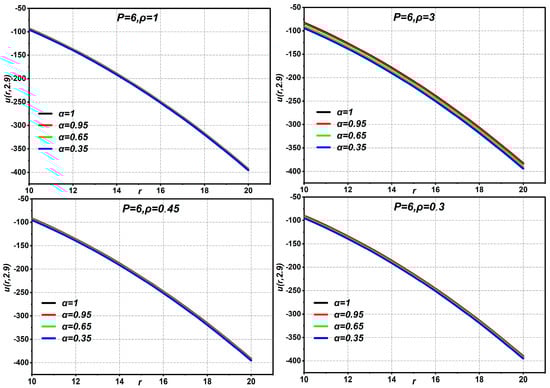
Figure 6. The graphs of Equation (28) displaying different values of parameters $\rho$ $\mathrm{with}a=0;\alpha =1;\alpha =0.95;\alpha =0.65;\alpha =0.35;r=10:1:20;P=6$.

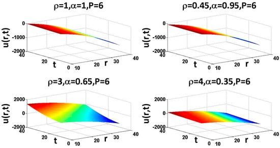
Figure 7. Surface shows the behavior of solution $U\left(r,t\right)$ of application 4.1 using Equation (28) with respect to $t$ and $r$, with $\left(\rho =1,\alpha =1\right),\left(\rho =0.45,\alpha =0.95\right),\left(\rho =3,\alpha =0.65\right),\left(\rho =4,\alpha =0.35\right)$.

4.2. Second Application

Consider the following time-fractional Navier–Stokes equation in cylindrical coordinates [29,30,31], given by Equation (1) with $P=0$ This is

$${}_t{}^{CK}{\mathcal{D}}_a^{\alpha ,\rho }U\left(r,t\right)={\rho }_0\left({\displaystyle \frac{{\partial }^{2}U}{{\partial r}^2}}+{\displaystyle \frac{1}{r}}{\displaystyle \frac{\partial U}{\partial r}}\right),\left(r,t\right)\in \mathsf{\Omega }\times \left(0,T\right),0<\alpha \le 1,$$

(30)

with the initial condition

$$U\left(r,0\right)=r,$$

(31)

Applying the HAM on both sides of Equation (30), and considering the initial condition provided by Equation (31), it is practical to select the first guess as follows:

$$U_0\left(r,0\right)=r,$$

(32)

we obtain

$$\mathcal{N}\left[\phi \left(r,t;p\right)\right]={}_t{}^{CK}{\mathcal{D}}_a^{\alpha ,\rho }\left[\phi \left(r,t;p\right)\right]-{\rho }_0\left({\displaystyle \frac{{\partial }^2}{{\partial r}^2}}\phi \left(r,t;p\right)+{\displaystyle \frac{1}{r}}{\displaystyle \frac{\partial }{\partial r}}\phi \left(r,t;p\right)\right).$$

(33)

Using Equation (33) and the assumption $G\left(r,t\right)=1$, we construct the zero-order deformation equations:

$$\left(1-p\right)\mathcal{D}\left[\phi \left(r,t;p\right)-U_0\left(r,t\right)\right]=ph\mathcal{N}\left[\phi \left(r,t;p\right)\right].$$

(34)

Naturally, if $P=0$ and $p=1$, we obtain $\phi \left(r,t;p=0\right)=U_0\left(r,t\right),$ and $\phi \left(r,t;p=1\right)=U\left(r,t\right),$ correspondingly.

Thus, the equation for nth-order deformation is as follows:

$$\mathcal{D}\left[U_n\left(r,t\right)-{{\delta }_{n}U}_{n-1}\left(r,t\right)\right]=h{\mathcal{R}}_n\left(U_{n-1},r,t\right).$$

(35)

Subject to the initial condition $U_n\left(r,a\right)=0$, where Equation (17) defines ${\delta }_n$ and

$$\mathcal{N}\left(U_{n-1},r,t\right)={}_t{}^{CK}{\mathcal{D}}_a^{\alpha ,\rho }\left[U_{n-1}\left(r,t\right)\right]-{\rho }_0\left({\displaystyle \frac{{\partial }^2}{{\partial r}^2}}{U}_{n-1}\left(r,t\right)+{\displaystyle \frac{1}{r}}{\displaystyle \frac{\partial }{\partial r}}{U}_{n-1}\left(r,t\right)\right).$$

The integral fractional operator ${\mathcal{I}}_a^{\alpha ;\rho }$ is now applied to both sides of Equation (24), giving us the following:

$${\mathcal{I}}_0^{\alpha ;\rho }{}_t{}^{CK}{\mathcal{D}}_a^{\alpha ,\rho }\left[U_n\left(r,t\right)-{{\delta }_{n}U}_{n-1}\left(r,t\right)\right]=h{\mathcal{I}}_a^{\alpha ;\rho }\left[{}_t{}^{CK}{\mathcal{D}}_a^{\alpha ,\rho }{U}_{n-1}\left(r,t\right)\right]-{\rho }_0\left({\displaystyle \frac{{\partial }^2}{{\partial r}^2}}{U}_{n-1}\left(r,t\right)+{\displaystyle \frac{1}{r}}{\displaystyle \frac{\partial }{\partial r}}{U}_{n-1}\left(r,t\right)\right),$$

(36)

From the initial guess of Equations (32) and (36), we obtain

$$\begin{gathered} U_0\left(r,t\right)=r, \\ {U}_1\left(r,t\right)=-h{{\rho }_0\mathcal{I}}_a^{\alpha ;\rho }\left[\left({\displaystyle \frac{{\partial }^2}{{\partial r}^2}}{U}_0\left(r,t\right)+{\displaystyle \frac{1}{r}}{\displaystyle \frac{\partial }{\partial r}}{U}_0\left(r,t\right)\right)\right]={\displaystyle \frac{-h{\rho }_0}{r}}{\displaystyle \frac{{\left(\frac{t^{\rho }-a^{\rho }}{\rho }\right)}^{\alpha }}{\Gamma \left(\alpha +1\right)}}, \\ {U}_2\left(r,t\right)=\left(1+h\right)U_1\left(r,t\right)-h{{\rho }_0\mathcal{I}}_a^{\alpha ;\rho }\left[\left({\displaystyle \frac{{\partial }^2}{{\partial r}^2}}{U}_1\left(r,t\right)+{\displaystyle \frac{1}{r}}{\displaystyle \frac{\partial }{\partial r}}{U}_1\left(r,t\right)\right)\right] \\ =-\left(1+h\right){\displaystyle \frac{h{\rho }_0}{r}}{\displaystyle \frac{{\left(\frac{t^{\rho }-a^{\rho }}{\rho }\right)}^{\alpha }}{\Gamma \left(\alpha +1\right)}}+{\displaystyle \frac{h^2{\rho }_0^2}{r^3}}{\displaystyle \frac{{\left(\frac{t^{\rho }-a^{\rho }}{\rho }\right)}^{2\alpha }}{\Gamma \left(2\alpha +1\right)}}, \\ {U}_3\left(r,t\right)=\left(1+h\right)U_2\left(r,t\right)-h{{\rho }_0\mathcal{I}}_a^{\alpha ;\rho }\left[\left({\displaystyle \frac{{\partial }^2}{{\partial r}^2}}{U}_2\left(r,t\right)+{\displaystyle \frac{1}{r}}{\displaystyle \frac{\partial }{\partial r}}{U}_2\left(r,t\right)\right)\right] \\ =-{\left(1+h\right)}^2{\displaystyle \frac{h{\rho }_0}{r}}{\displaystyle \frac{{\left(\frac{t^{\rho }-a^{\rho }}{\rho }\right)}^{\alpha }}{\Gamma \left(\alpha +1\right)}}+2\left(1+h\right){\displaystyle \frac{h^2{\rho }_0^2}{r^3}}{\displaystyle \frac{{\left(\frac{t^{\rho }-a^{\rho }}{\rho }\right)}^{2\alpha }}{\Gamma \left(2\alpha +1\right)}}-9{\displaystyle \frac{h^3{\rho }_0^3}{r^5}}{\displaystyle \frac{{\left(\frac{t^{\rho }-a^{\rho }}{\rho }\right)}^{3\alpha }}{\Gamma \left(3\alpha +1\right)}}, \\ ⋮ \end{gathered}$$

A precise approximation of Equation (30) is provided by the following:

$$\begin{gathered} U\left(r,t\right)=U_0\left(r,t\right)+U_1\left(r,t\right)+U_2\left(r,t\right){+U}_3\left(r,t\right)+\cdots \\ =r-{\displaystyle \frac{h{\rho }_0}{r}}{\displaystyle \frac{{\left(\frac{t^{\rho }-a^{\rho }}{\rho }\right)}^{\alpha }}{\Gamma \left(\alpha +1\right)}}\left[1+\left(1+h\right)+{\left(1+h\right)}^2+{\left(1+h\right)}^3+\cdots \right] \\ +{\displaystyle \frac{h^2{\rho }_0^2}{r^3}}{\displaystyle \frac{{\left(\frac{t^{\rho }-a^{\rho }}{\rho }\right)}^{2\alpha }}{\Gamma \left(2\alpha +1\right)}}\left[1+2\left(1+h\right)+{3\left(1+h\right)}^2+4{\left(1+h\right)}^3+\cdots \right] \\ -9{\displaystyle \frac{h^3{\rho }_0^3}{r^5}}{\displaystyle \frac{{\left(\frac{t^{\rho }-a^{\rho }}{\rho }\right)}^{3\alpha }}{\Gamma \left(3\alpha +1\right)}}\left[1+3\left(1+h\right)+{6\left(1+h\right)}^2+{10\left(1+h\right)}^3+\cdots \right]+\cdots \end{gathered}$$

It is important to note that HAM has great freedom to choose the auxiliary linear operator, the initial guess, and the auxiliary parameters $h$. When we choose $h=-1$ and ${\rho }_0=1$ in the above equation, the results are as follows:

$$\begin{gathered} U\left(r,t\right)=r+{\displaystyle \frac{1}{r}}{\displaystyle \frac{{\left(\frac{t^{\rho }-a^{\rho }}{\rho }\right)}^{\alpha }}{\Gamma \left(\alpha +1\right)}}+{\displaystyle \frac{1}{r^3}}{\displaystyle \frac{{\left(\frac{t^{\rho }-a^{\rho }}{\rho }\right)}^{2\alpha }}{\Gamma \left(2\alpha +1\right)}}+{\displaystyle \frac{9}{r^5}}{\displaystyle \frac{{\left(\frac{t^{\rho }-a^{\rho }}{\rho }\right)}^{3\alpha }}{\Gamma \left(3\alpha +1\right)}}+{\displaystyle \frac{225}{r^7}}{\displaystyle \frac{{\left(\frac{t^{\rho }-a^{\rho }}{\rho }\right)}^{4\alpha }}{\Gamma \left(4\alpha +1\right)}}\dots . \\ =r+\sum _{k=1}^{\infty }{\displaystyle \frac{1\times 3^2\times 5^2\times \dots \times {\left(2k-3\right)}^2}{r^{2k-1}}}{\displaystyle \frac{{\left(\frac{t^{\rho }-a^{\rho }}{\rho }\right)}^{k\alpha }}{\Gamma \left(k\alpha +1\right)}} \\ =r+\sum _{k=1}^n{\displaystyle \frac{{{\prod }_{i=1}^k\left(2i-3\right)}^2}{r^{2k-1}}}{\displaystyle \frac{{\left(\frac{t^{\rho }-a^{\rho }}{\rho }\right)}^{k\alpha }}{\Gamma \left(k\alpha +1\right)}}. \end{gathered}$$

(37)

This is an exact solution. Note that there is no relationship between $h$ and the series. For Equations (30) and (31), there are noteworthy exceptional instances. Substituting $a=0$ and $\rho =1$ into (37), we obtain the solution of Equation (30) under Riemann–Liouville memory:

$$U\left(r,t\right)=r+\sum _{k=1}^{\infty }{\displaystyle \frac{1\times 3^2\times 5^2\times \dots \times {\left(2k-3\right)}^2}{r^{2k-1}}}{\displaystyle \frac{t^{k\alpha }}{\Gamma \left(k\alpha +1\right)}}.$$

(38)

Equation (38) provides the same solution as that derived by Oliveira et al. using HAM [21], Momani et al. using ADM [30], Ragab et al. [31] using HAM, and Bairwa et al. [29] using the iterative Laplace transform. The fourth-approximate HAM solution to the Navier–Stokes equation with time-fractional derivatives in Example 2 is given in Figure 8, Figure 9, Figure 10, Figure 11 and Figure 12 for different values of $\alpha \mathrm{and}\rho$. The statistics show that while fluid at low speed increases with increasing pipe radius or flow duration over time, fluid flow speed decreases with increasing fractional order. In Figure 8, Figure 9, Figure 10 and Figure 11, the data show that increasing the fractional order of both $\alpha \mathrm{and}\rho$ leads to a decrease in the fluid flow velocity, while increasing the pipe radius or flow duration over time leads to an increase in the fluid flow velocity.

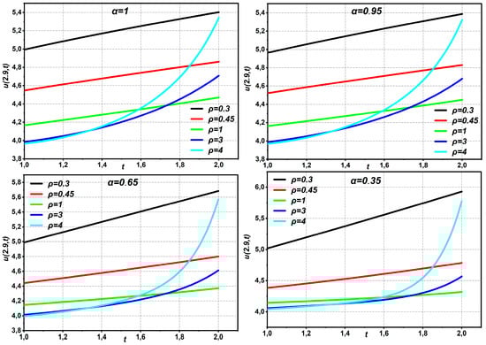
Figure 8. The graphs of Equation (37) displaying different values of parameters $\rho$ with $a=0;\alpha =1;\alpha =0.95;\alpha =0.65;\alpha =0.35$.

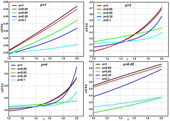
Figure 9. The graphs of Equation (37) displaying different values of parameters $\alpha$ with $a=0;\rho =1;\rho =3;\rho =4;\rho =0.45$.

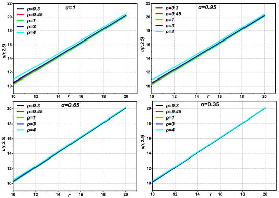
Figure 10. The graphs of Equation (37) displaying different values of parameters $\alpha$ with $a=0;\rho =1;\rho =3;\rho =4;\rho =0.45;\rho =0.3;r=10:1:20;t=2.5$.

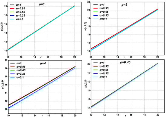
Figure 11. The graphs of Equation (37) displaying different values of parameters $\rho$ with $a=0;\alpha =1;\alpha =0.95;\alpha =0.65;\alpha =0.35;\alpha =\mathrm{0,1};r=10:1:20;t=2.5$.

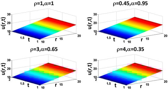
Figure 12. Surface shows the behavior of solution $U\left(r,t\right)$ of application 4.2 using Equation (37), with respect to $t$ and $r$, with $\left(\rho =1,\alpha =1\right),\left(\rho =0.45,\alpha =0.95\right),\left(\rho =3,\alpha =0.65\right),\left(\rho =4,\alpha =0.35\right)$.

5. Discussion

Several analytical and semi-analytical methods have been developed to solve time-fractional Navier–Stokes (NS) equations, highlighting the growing importance of fractional calculus in modeling complex fluid flows. For instance, Oliveira et al. [21] applied the HAM to time-fractional NS equations involving $\psi$-Caputo derivatives, revealing the method’s flexibility in accommodating generalized operators. Momani et al. [30] employed the Adomian Decomposition Method (ADM), providing a foundational comparison of analytical techniques for time-fractional models. Similarly, Bairwa et al. [29] used an iterative Laplace transform approach to obtain solutions for the NS equations, showing strong agreement with the analytical results obtained using the homotopy analysis method.

More recent efforts have expanded these methods through hybrid approaches. Alqahtani et al. [28] integrated homotopy perturbation with Laplace transforms to solve Caputo-type fractional NS equations, demonstrating improved convergence and computational stability. In a comparable direction, Sripacharasakullert et al. [32] employed the homotopy perturbation method alongside fractional multidimensional Burgers equations, indicating strong performance in nonlinear systems. These contributions underline the adaptability of homotopy-based techniques in addressing fractional differential equations.

With a careful look and comparative analysis, we conclude the following:

Unlike most of the above, the present work introduces the Caputo–Katugampola derivative, a generalized operator that unifies several classical fractional derivatives, and applies it in tandem with the HAM. This combination provides not only analytical tractability but also enhanced modeling flexibility via the parameter ρ, which controls the memory behavior of the system. Furthermore, we provide exact closed-form solutions and perform a convergence analysis that complements and extends prior studies, particularly those by Ragab et al. [31], Oliveira et al. [21], and W. Sawangtong et al. [33]. Equations (30) and (37), obtained by the HAM method, provide the analytical solution to the time-fractional Navier–Stokes equations, which can be expressed in terms of the parameter $\rho$. Thus, the fluid flow in the pipe is affected by the fractional order $\alpha$ and the parameter $\rho$ of the fractional Katogambola derivative expressed by the Caputo formula. Variations in these parameters affect the fluid flow characteristics inside the pipe, as discussed in the section on “applications of HAM on time-fractional Navier–Stokes equations”.

6. Conclusions

In this study, we have developed an analytical framework for solving the time-fractional Navier–Stokes equations in cylindrical coordinates using the HAM in conjunction with the Caputo–Katugampola fractional derivative. The approach allows the derivation of exact and convergent series solutions for two initial value problems under different flow profiles.

Our analysis reveals the critical influence of the fractional order $\alpha$ and the parameter $\rho$ on the velocity field. The flexibility of the Caputo–Katugampola derivative enables modeling a wide class of fractional behaviors, while HAM provides convergence control through an auxiliary parameter. The derived solutions reduce to known results in special cases, confirming the correctness and robustness of the method.

Graphical simulations further highlight the transition in flow behavior as $\alpha and\rho$ vary, demonstrating the sensitivity and adaptability of the fractional model. These insights can inform future studies in fractional fluid mechanics. The techniques and results presented herein offer a promising direction for further exploration of nonlinear fractional differential equations in both theoretical and applied contexts. Future work aims to develop solutions capable of handling practical applications in fields such as fluid dynamics, biomedical engineering, and environmental engineering.

References

- Herrmann, R. Fractional Calculus: An Introduction for Physicists; World Scientific Publishing Company: Singapore, 2011. [Google Scholar] [CrossRef]
- Kiryakova, V. Generalized Fractional Calculus and Applications; John Willey & Sons: New York, NY, USA, 1994; Available online: https://books.google.dz/books?id=RvcONCIkFwoC (accessed on 9 October 2025).
- Miller, K.S.; Ross, B. An Introduction to the Fractional Calculus and Differential Equations; Willey: New York, NY, USA, 1993. Available online: https://lccn.loc.gov/93009500 (accessed on 9 October 2025).
- Kilbas, A.A.; Srivastava, H.M.; Trujillo, J.J. Theory and Applications of Fractional Differential Equations; Elsevier: Amsterdam, The Netherlands, 2006; Available online: https://worldcat.org/title/1025236735 (accessed on 9 October 2025).
- Podlubny, I. Fractional Differential Equations: An Introduction to Fractional Derivatives, Fractional Differential Equations, to Methods of Their Solution and Some of Their Applications; Academic Press: San Diego, CA, USA, 1999; Available online: https://www.scirp.org/reference/referencespapers?referenceid=1689024 (accessed on 9 October 2025).
- Alqahtani, A.M.; Mihoubi, H. Analytical Solutions for Fractional Black-Scholes European Option Pricing Equation by Using Homotopy Perturbation Method with Caputo Fractional Derivative. Math. Model. Eng. Probl. 2025, 12, 1562–1570. [Google Scholar] [CrossRef]
- Zuo, J.; Liu, C.; Vetro, C. Normalized solutions to the fractional Schrödinger equation with potential Mediterr. J. Math. 2023, 20, 216. [Google Scholar] [CrossRef]
- Zuo, J.; An, T.; Ye, G.; Qiao, Z. Nonhomogeneous fractional p-Kirchhoff problems involving a critical nonlinearity. Electron J. Qual. Theory Differ. Equ. 2019, 41, 1–15. [Google Scholar] [CrossRef]
- Öziş, T.; Ağırseven, D. He’s homotopy perturbation method for solving heat-like and wave-like equations with variable coefficients. Phys. Lett. A 2008, 372, 5944–5950. [Google Scholar] [CrossRef]
- Jena, R.M.; Chakraverty, S. Solving time-fractional Navier–Stokes equations using homotopy perturbation Elzaki transform. SN Appl. Sci. 2019, 116, 16. [Google Scholar] [CrossRef]
- Liao, S. Beyond Perturbation: Introduction to the Homotopy Analysis Method, 1st ed.; Chapman and Hall/CRC: Boca Raton, FL, USA, 2003. [Google Scholar] [CrossRef]
- Barkat, O.; Alqahtani, A.M. Analytical solutions for fractional Navier–Stokes equation Using residual power series with ϕ-Caputo generalized fractional derivative. AIMS Math. 2025, 10, 15476–15496. [Google Scholar] [CrossRef]
- Bakicierler, G.; Alfaqeih, S.; Mısırlı, E. Application of the modified simple equation method for solving two nonlinear time-fractional long water wave equations. Rev. Mex. Física 2021, 67, 825–831. [Google Scholar] [CrossRef]
- Abazari, R.; Soltanalizadeh, B. Reduced differential transform method its application on Kawahara equations. Thai J. Math. 2000, 11, 199–216. [Google Scholar]
- Keskin, Y.; Oturanc, G. The Reduced differential transform method: A new approach to fractional partial differential equations. Nonlinear Sci. Lett. A 2010, 1, 207–217. [Google Scholar]
- Liao, S. A Kind of Linearity-Invariance Under Homotopy and Some Simpla Applications of It in Mechanics; Technische Universität Hamburg-Harburg: Hamburg, Germany, 1992. [Google Scholar]
- Liao, S. An approximate solution technique not depending on small parameters: A special example, International. J. Linear Mech. 1995, 30, 371–380. [Google Scholar] [CrossRef]
- Podlubny, I.; Chechkin, A.; Skovranek, T.; Chen, Y.; Vinagre, B. Matrix approach to discrete fractional calculus II: Partial fractional differential equations. J. Comput. Phys. 2009, 228, 3137–3153. [Google Scholar] [CrossRef]
- Zhang, X.; Tang, B.; He, Y. Homotopy analysis method for higher-order fractional integro-differential equations. Comput. Math. Appl. 2011, 62, 3194–3203. [Google Scholar] [CrossRef]
- Sakar, M.G.; Erdogan, F. The homotopy analysis method for solving the timefractional Fornberg–Whitham equation and comparison with Adomian’s decomposition method. Appl. Math. Model. 2013, 37, 8876–8885. [Google Scholar] [CrossRef]
- Oliveira, D.S.; de Oliveira, E.C. Analytical solutions for Navier–Stokes equations with Caputo fractional derivative. SeMA J. 2021, 78, 137–154. [Google Scholar] [CrossRef]
- Mihoubi, H.; Alqahtani, A.M.; Arioua, Y.; Bouderah, B.; Tayebi, T. Homotopy Perturbationρ-Laplace Transform Approach for Numerical Simulation of Fractional Navier-Stokes Equations. Contemp. Math. 2025, 6, 2878–2906. [Google Scholar] [CrossRef]
- Chakraverty, S.; Jena, R.M.; Jena, S.K. Computational Fractional Dynamical Systems, Fractional Differential Equations and Applications; Wiley: Hoboken, NJ, USA, 2022; Available online: https://books.google.dz/books?id=YAKUEAAAQBAJ (accessed on 9 October 2025).
- U.N. Katugampola. New approach to a generalized fractional integral. Appl. Math. Comput. 2011, 218, 860–865. [Google Scholar]
- U.N. Katugampola. New approach to a generalized fractional derivatives. Bull. Math. Anal. Appl. 2014, 6, 1–15. [Google Scholar]
- Lupinska, B. Properties of the Katugampola fractional operators. Tatra Mt. Math. Publ. 2021, 79, 135–148. [Google Scholar] [CrossRef]
- Chowdhury, M.S.H.; Hashim, I.; Abdulaziz, O. Comparison of homotopy analysis method and homotopy perturbation method for purely nonlinear fin-type problems. Commun. Nonlinear Sci. Numer. Simul. 2009, 14, 371–378. [Google Scholar] [CrossRef]
- Alqahtani, A.M.; Mihoubi, H.; Arioua, Y.; Bouderah, B. Analytical Solutions of Time-Fractional Navier–Stokes Equations Employing Homotopy Perturbation–Laplace Transform Method. Fractal Fract. 2024, 2024, 23. [Google Scholar] [CrossRef]
- Bairwa, R.K.; Singh, J. Analytical approach to fractional Navier-Stokes equations by iterative Laplace transform method. In International Workshop of Mathematical Modelling, Applied Analysis and Computation; Springer: Singapore, 2018; Volume 272, pp. 179–188. [Google Scholar] [CrossRef]
- Momani, S.; Odibat, Z. Analytical solution of a time-fractional Navier–Stokes equation by Adomian decomposition method. Appl. Math. Comput. 2006, 177, 488–494. [Google Scholar] [CrossRef]
- Ragab, A.A.; Hemida, K.M.; Mohamed, M.S.; El Salam, M.A.A. Solution of time-fractional Navier-Stokes equation by using homotopy analysis method. Gen. Math. Notes 2012, 13, 13–21. [Google Scholar]
- Sripacharasakullert, P.; Sawangtong, W.; Sawangtong, P. An approximate analytical solution of the fractional multi-dimensional Burgers equation by the homotopy perturbation method. Adv. Differ. Equ. 2019, 1, 1–12. [Google Scholar] [CrossRef]
- Sawangtong, W.; Dunnimit, P.; Wiwatanapataphe, B.; Sawangtong, P. An analytical solution to the time fractional Navier–Stokes equation based on the Katugampola derivative in Caputo sense by the generalized Shehu residual power series approach. Partial. Differ. Equ. Appl. Math. 2024, 11, 100890. [Google Scholar] [CrossRef]
Disclaimer/Publisher’s Note: The statements, opinions and data contained in all publications are solely those of the individual author(s) and contributor(s) and not of MDPI and/or the editor(s). MDPI and/or the editor(s) disclaim responsibility for any injury to people or property resulting from any ideas, methods, instructions or products referred to in the content. |
© 2025 by the authors. Licensee MDPI, Basel, Switzerland. This article is an open access article distributed under the terms and conditions of the Creative Commons Attribution (CC BY) license (https://creativecommons.org/licenses/by/4.0/).