An Efficient Algorithm for Basic Elementary Matrix Functions with Specified Accuracy and Application

Abstract

If the matrix function $f\left(At\right)$ posses the properties of $f\left(At\right)=g\left(f(\left(\frac{t}{k}A\right)\right)$, then the recurrence formula $f_{i-1}=g\left(f_i\right),i=N,N-1,\cdots ,1,f\left(tA\right)=f_0$, can be established. Here, $f_N=f\left(A_N\right)={\displaystyle \sum _{j=0}^m}{a}_j{A}_N^j,A_N=\frac{t}{k^N}A$. This provides an algorithm for computing the matrix function $f\left(At\right)$. By specifying the calculation accuracy p, a method is presented to determine m and N in a way that minimizes the time of the above algorithm, thus providing a fast algorithm for $f\left(At\right)$. It is important to note that m only depends on the calculation accuracy p and is independent of the matrix A and t. Therefore, $f\left(A_N\right)$ has a fixed calculation format that is easily computed. On the other hand, N depends not only on A, but also on t. This provides a means to select t such that N is equal to 0, a property of significance. In summary, the algorithm proposed in this article enables users to establish a desired level of accuracy and then utilize it to select the appropriate values for m and N to minimize computation time. This approach ensures that both accuracy and efficiency are addressed concurrently. We develop a general algorithm, then apply it to the exponential, trigonometric, and logarithmic matrix functions, and compare the performance with that of the internal system functions of Mathematica and Pade approximation. In the last section, an example is provided to illustrate the rapid computation of numerical solutions for linear differential equations.

1. Introduction

Matrix exponent functions plays a crucial role in various fields, including ordinary differential equations and control theory. In particular, they are instrumental in analyzing general structural dynamic systems, represented by the initial value problem:

$$\begin{array}{c}Mx″+Gx\prime +Kx=r\left(t\right),x\left(0\right)=x_0,x\prime \left(0\right)=x_1,\end{array}$$

(1)

where $M,G$, and K are n by n square matrices, and $r\left(t\right)$ denotes the external force applied. The introduction of dual variables of a Hamiltonian system,

$$\begin{array}{c}p=Mx\prime +Gx/2,\end{array}$$

(2)

results in the following system:

$$\begin{array}{c}U\prime =HU+F\left(t\right),U\left(0\right)=U_0,\end{array}$$

(3)

where

$$\begin{array}{c}U=\left(\begin{array}{c}q\\ p\end{array}\right),H=\left(\begin{array}{cc}-M^{-1}G/2& M^{-1}\\ G{M}^{-1}G/4-K& -M^{-1}G/2\end{array}\right),\\ F\left(t\right)=\left(\begin{array}{c}0\\ r\left(t\right)\end{array}\right),q=x,U_0=\left(\begin{array}{c}{x}_0\\ M{x}_1+G{x}_0/2\end{array}\right).\end{array}$$

(4)

The solution of (3) is provided as follows:

$$\begin{array}{c}U\left(t\right)=e^{Ht}{U}_0+{\int }_0^t{e}^{H(t-s)}F\left(s\right)ds.\end{array}$$

(5)

When a problem is oscillatory, the formal solution often involves both the sine and cosine of a matrix. Famous examples include the Schr$\stackrel{”}{\mathrm{o}}$dinger equation in quantum mechanics:

$$\begin{array}{c}i\frac{d\psi }{dt}=H\left(t\right)\psi ,\psi \left(t_0\right)={\psi }_0,\end{array}$$

(6)

where $H\left(t\right)$ is a Hermitian operator and $\psi$ is a complex wave function. If $H\left(t\right)=A$ is a real and constant matrix, the solution of (6) is as follows:

$$\begin{array}{c}\psi \left(t\right)=e^{-iAt}{\psi }_0=\left(cos\left(tA\right)-isin\left(tA\right)\right){\psi }_0.\end{array}$$

(7)

There are other examples where the computation of the sine and cosine of a matrix can be of interest. Wave equations provided by the generic second order system are written as follows:

$$\begin{array}{c}x″+Kx=F\left(t\right),x\left(0\right)=x_0,x\prime \left(0\right)=x_1,\end{array}$$

(8)

where the solution is provided by the variation of the constant method:

$$\begin{array}{c}x\left(t\right)=cos\left(tA\right)x_0+{sin}_1\left(tA\right)x_1+{\int }_0^t{sin}_1\left((t-s)A\right)F\left(s\right)ds,\end{array}$$

(9)

where $A=\sqrt{K},{sin}_1\left(tA\right)={\int }_0^{t}cos\left(sA\right)ds.$ If A is invertible, then (9) can be written as follows:

$$\begin{array}{c}x\left(t\right)=cos\left(tA\right)x_0+sin\left(tA\right)A^{-1}{x}_1+A^{-1}{\int }_0^{t}sin\left((t-s)A\right)F\left(s\right)ds.\end{array}$$

(10)

For (5), providing $U\left(k\tau \right)(k=1,2,\cdots )$ as accurately as possible is a concern for engineers and mathematicians, where $\tau$ is called the step. The specific method for this problem is as follows:

$$\begin{array}{c}{U}_k=T{U}_{k-1}+{\int }_0^{\tau }{e}^{Hs}F(k\tau -s)ds,k=1,2,\cdots ,T=e^{H\tau }.\end{array}$$

(11)

Similarly, for (10), providing the algorithm $x\left(k\tau \right)(k=1,2,\cdots )$ as accurately as possible involves introducing vectors $x\prime =y$ and the following algorithm:

$$\begin{array}{c}{x}_k=cos\left(\tau A\right)x_{k-1}+sin\left(\tau A\right)A^{-1}{y}_{k-1}+A^{-1}{\int }_0^{\tau }sin\left(sA\right)F(k\tau -s)ds,\hfill \\ y_k=-Asin\left(\tau A\right)x_{k-1}+cos\left(\tau A\right)y_{k-1}+{\int }_0^{\tau }cos\left(sA\right)F(k\tau -s)ds,\hfill \\ x_0=x\left(0\right),y_0=x\prime \left(0\right)=x_1.\hfill \end{array}$$

(12)

To improve the accuracy of $U\left(k\tau \right)$ and $x\left(k\tau \right)$, it is essential to develop an algorithm with high accuracy for computing $T=e^{H\tau },cos\left(\tau A\right)$ and $sin\left(\tau A\right)$ and the integral containing these matrix functions. This paper improves the algorithms developed for the computation of $e^A$ and $cosA$ in the existing literature, see [1,2,3,4,5,6,7,8,9,10,11,12,13,14,15], and also discusses the computation of other trigonometric, hyperbolic, logarithmic, and related inverse triangular and inverse hyperbolic matrices.

2. The General Theorem of the Fast Algorithm for Matrix Functions

In [16], we addressed the challenge of rapidly calculating elementary functions with specified precision. The implementation method involves an analytic function $f\left(x\right)$ specifying property,

$$f\left(x\right)=g\left(f\left(\frac{x}{k}\right)\right),\mathrm{where}k>1.$$

(13)

If $C_0$ is an approximation as close as possible to $f\left(\frac{x}{k^N}\right),$ with N as a positive integer, for example,

$$\begin{array}{c}{C}_0=\sum _{j=0}^m\frac{f^{\left(j\right)}\left(0\right){\left(\Delta x\right)}^j}{j!},\Delta x=\frac{x}{k^N},m=1,2,\cdots \end{array}$$

(14)

or $C_0$ being the Padé approximation of $f\left(\frac{x}{k^N}\right),$ then the following calculations are performed:

$$\begin{array}{c}\mathrm{for}(i=0,i<N,i++)C_{i+1}=g\left(C_i\right).\end{array}$$

(15)

Completing (14) and (15), $f\left(x\right)\approx C_N$ is obtained. This method is also applicable to the calculation of matrix functions, where the variable x is replaced by the n by n square matrix $A.$ Now, we have the following:

$$\begin{array}{c}{C}_0=\sum _{j=0}^m\frac{f^{\left(j\right)}\left(0\right){\left(\Delta A\right)}^j}{j!},\Delta A=\frac{1}{k^N}A,m=1,2,\cdots \end{array}$$

(16)

or $C_0$ is the Padé approximation of $f\left(\Delta A\right).$ Our objective is to determine m and N to minimize the computation time under the condition that the truncation error and computational precision are ${10}^{-p}$. For the matrix function calculation, the coefficient calculation of (14) can be ignored, mainly focusing on the multiplication calculation of the matrix in (16) and (15). If the number of multiplications to complete $g\left(A\right)$ is K, then the total number of times to complete (16) and (15) is roughly

$$\begin{array}{c}q(m,N)=(m+KN)M_n,\end{array}$$

(17)

where $M_n$ is the number of times to complete one multiplication of the n by n matrix. Based on the above discussion, we present a fast algorithm for the matrix function as follows.

Theorem  1.

Let $m_p$ be an integer close to the minimum point of $h\left(m\right)$, where

$$\begin{array}{c}h\left(m\right)=m+\frac{pKln10}{(m+1)lnk}+\frac{K}{(m+1)lnk}ln\left|\frac{f^{(m+1)}\left(0\right)}{(m+1)!}\right|\end{array}$$

(18)

and

$$\begin{array}{c}N=\left[\frac{pln10}{(m+1)lnk}+\frac{1}{(m+1)lnk}ln\left|\frac{f^{(m+1)}\left(0\right)}{(m+1)!}\right|+\frac{ln∥A∥}{lnk}\right]+1.\end{array}$$

(19)

(1) $C_0={\sum }_{j=0}^{m_p}\frac{f^{\left(j\right)}\left(0\right){\left(\Delta A\right)}^j}{j!}$, where $\Delta A=\frac{1}{k^N}A,$ or $C_0$ is a Padé approximation of $f\left(\Delta A\right).$

(2) for($i=0,i<N,i++$) $C_{i+1}=g\left(C_i\right)$ and $\left(A\right)\approx C_N.$

The above algorithm is a fast algorithm for the general matrix function.

Proof. 

With a truncation error of ${10}^{-p}$, for (16) to be satisfied,

$$\begin{array}{c}∥\frac{f^{(m+1)}\left(0\right){\left(\Delta A\right)}^{m+1}}{(m+1)!}∥=\left|\frac{f^{(m+1)}\left(0\right)}{(m+1)!k^{(m+1)N}}\right|∥A^{m+1}∥\le \left|\frac{f^{(m+1)}\left(0\right)}{(m+1)!k^{(m+1)N}}\right|{∥A∥}^{m+1}<{10}^{-p},\end{array}$$

(20)

where $∥A∥$ is a norm of $A.$ So,

$$\begin{array}{c}N>\frac{pln10}{(m+1)lnk}+\frac{1}{(m+1)lnk}ln\left|\frac{f^{(m+1)}\left(0\right)}{(m+1)!}\right|+\frac{ln∥A∥}{lnk}.\end{array}$$

(21)

From (17), we obtain the following:

$$\begin{array}{c}q(m,N)>g\left(m\right)=\left(m+\frac{pKln10}{(m+1)lnk}+\frac{K}{(m+1)lnk}ln\left|\frac{f^{(m+1)}\left(0\right)}{(m+1)!}\right|+\frac{Kln∥A∥}{lnk}\right)M_n.\end{array}$$

(22)

Note that the minimum point of $g\left(m\right)$ has nothing to do with $\frac{Kln∥A∥}{lnk}$. By making $q(m,N)$ as small as possible, the algorithm obtained by (1) and (2) is a fast algorithm, thus completing the proof of the theorem. □

Remark  1.

In the specific calculation, $∥A∥$ can be replaced by the approximate eigenvalue with the maximum modulus in this paper.

$$\begin{array}{c}\left|\frac{f^{(m+1)}\left(0\right)}{(m+1)!k^{(m+1)N}}\right|{∥A∥}^{m+1}<{10}^{-p}.\end{array}$$

(23)

3. Fast Algorithm for ${\mathit{e}}^{\mathit{A}},\mathbf{cos}\mathit{A},\mathbf{sin}\mathit{A},\mathbf{sinh}\mathit{A},$ and $\mathbf{cosh}\mathit{A}$

Suppose $\lambda =∥A∥$ is a norm for A. If we let $A=\lambda A_0,$ then $∥A_0∥\le 1$. From (19), we can obtain the following:

$$\begin{array}{c}{N}_p=\left[\frac{pln10}{(m+1)lnk}+\frac{1}{(m+1)lnk}ln\left|\frac{f^{(m+1)}\left(0\right)}{(m+1)!}\right|+\frac{ln\lambda }{Klnk}\right]+1.\end{array}$$

(24)

In order to reduce the length of the article, the algorithms for several matrix functions are compiled into a table.

Theorem  2.

For $e^A,cosA,sinA,coshA$, and $sinhA,$ we devised the following fast algorithm using Theorem 1.

Remark  2.

It is worth noting that $m_p$ in Table 1 only depends on the calculation accuracy p and the matrix function, and is independent of matrix A.

Table 1. The fast algorithm for $e^A,cosA,sinA,coshA,\mathrm{and}sinhA$.

	${\mathit{m}}_{\mathit{p}},{\mathit{N}}_{\mathit{p}}$	Algorithm
$e^A$	$m_p=\left[\sqrt{\frac{9pln10}{8ln2}}\right],N_p=\left[N_e\right]+1$	$\left(1\right)B=\frac{A}{2^{N_p}},C=I+{\sum }_{j=1}^{m_p}\frac{B^j}{j!}$
		$\left(2\right)for(i=0,i<N,i++)C=C^2$
		$\left(3\right)e^A=C$
$\left\{\begin{array}{c}sinA\\ sinhA\end{array}\right\}$	$m_p=\left[\sqrt{\frac{pln10}{2ln3}}\right],N_p=\left[N_{sin}\right]+1$	$\left(1\right)B=\frac{A^2}{3^{2N_p}},C=\frac{A}{3^N}+\frac{A}{3^N}{\sum }_{j=1}^{m_p}\frac{{(\mp B)}^j}{(2j+1)!}$
		$\left(2\right)for(i=0,i<N,i++)C=3C\mp 4C^3$
		$\left(3\right)\left\{\begin{array}{c}sinA\\ sinhA\end{array}\right\}=C$
$\left(I\right)\left\{\begin{array}{c}cosA\\ coshA\end{array}\right\}$	$m_p=\left[\sqrt{\frac{pln10}{2ln3}}\right]+1,N_p=\left[N_{sin}\right]$	$\left(1\right)B=\frac{A^2}{3^{2N_p}},C=I+{\sum }_{j=1}^{m_p}\frac{{(\mp B)}^j}{\left(2j\right)!}$
		$\left(2\right)for(i=0,i<N,i++)C=4C^3-3C$
		$\left(3\right)\left\{\begin{array}{c}cosA\\ coshA\end{array}\right\}=C$
$\left(II\right)\left\{\begin{array}{c}cosA\\ coshA\end{array}\right\}$	$m_p=\left[\sqrt{\frac{pln10}{2ln3}}\right]+1,N_p=\left[N_{sin}\right]$	$\left(1\right)B=\frac{A^2}{3^{2N_p}},C=I+{\sum }_{j=1}^{m_p}\frac{{(\mp B)}^j}{\left(2j\right)!}$
		$\left(2\right)for(i=0,i<N,i++)C=C^2-I$
		$\left(3\right)\left\{\begin{array}{c}cosA\\ coshA\end{array}\right\}=C$
$\begin{array}{c}{N}_e=\frac{pln10}{(m_p+1)ln2}+\frac{ln\lambda }{ln2}-\frac{ln(m_p+1)!}{(m_p+1)ln2},N_{cos}=\frac{pln10}{(2m_p+1)ln2}+\frac{ln\lambda }{ln2}-\frac{ln(2m_p+1)!}{(2m_p+1)ln2},\\ N_{sin}=\frac{pln10}{(2m_p+2)ln3}+\frac{ln\lambda }{ln3}-\frac{ln(2m_p+2)!}{(2m_p+2)ln3}.\end{array}$

Now, we utilize the general fast algorithm to specifically demonstrate the correctness of the algorithms in Table 1. The algorithms in Table 1 are straightforward; they involve placing the specific functions f and g into the general algorithm, and the tricky part lies in deriving the formulas of $m_p$ and $N_p.$ We calculate the formulas for $m_p$ and $N_p$ for the function $e^A$ for $12\le p\le 36$ here. In fact, the graphing of the function of $h\left(m\right)$ supports our results for all values of $p.$ The derivation of $m_p$ and $N_p$ for the other functions is very similar.

(1) For the function $e^A,$ we have $g\left(u\right)=u^2,k=2,K=1,$ and

$$\begin{array}{c}h\left(m\right)=m+\frac{pln10}{(m+1)ln2}-\frac{1}{(m+1)ln2}ln(m+1)!.\end{array}$$

(25)

Using Sterling’s approximation formula, we obtain the following:

$$ln((m+1)!)=\frac{1}{2}ln\left(2\pi \right)+\frac{1}{2}ln(m+1)+(m+1)ln(m+1)-m-1+O\left(\frac{1}{m+1}\right).$$

Now, implementing it into (25), we obtain the following:

$$h\left(m\right)\approx m+\frac{pln10}{(m+1)ln2}-\frac{ln\left(2\pi \right)}{2(m+1)ln2}-\frac{ln(m+1)}{2(m+1)ln2}+\frac{1}{ln2}.$$

Let

$$q\left(x\right)=x+\frac{pln10}{(x+1)ln2}-\frac{ln\left(2\pi \right)}{2(x+1)ln2}-\frac{ln(x+1)}{2(x+1)ln2}+\frac{1}{ln2}.$$

Taking its derivative with respect to $x,$ one obtains

$$q\prime \left(x\right)=1-\frac{pln10}{{(x+1)}^{2}ln2}+\frac{ln\left(2\pi \right)}{2{(x+1)}^{2}ln2}+\frac{ln(x+1)}{2{(x+1)}^{2}ln2}-\frac{1}{2{(x+1)}^{2}ln2}.$$

To determine extreme values, we set it to 0 and multiply both sides by ${(m+1)}^2:$

$${(x+1)}^2-\frac{1}{ln2}(x+1)+\frac{ln(x+1)}{2ln2}-\frac{2pln10-ln\left(2\pi \right)+1}{2ln2}=0.$$

Using simple algebra, we obtain the following:

$${(x+1)}^2>\frac{(m+1)-ln(m+1)+(m+1)-ln\left(2\pi \right)}{2ln2}+\frac{2pln10+1}{2ln2}>\frac{2pln10+1}{2ln2}.$$

Using $p=12,$ we obtain a lower bound for $x:$

$$x>\sqrt{\frac{2pln10+1}{2ln2}}-1=6.37.$$

Thus, we have a lower bound for m: $m\ge 6.$ We also can solve the quadratic equation to get

$$m+1=\frac{1}{ln2}+\sqrt{\frac{1}{4{ln}^{2}2}+\frac{8pln10-4ln\left(2\pi \right)+4}{8ln2}}.$$

Now, using the smallest value for m obtained and $p=36,$ we can obtain our first upper bound:

$$m<-1+\frac{1}{ln2}+\sqrt{\frac{1}{4{ln}^{2}2}-\frac{ln7}{2ln2}+\frac{276ln10-4ln\left(2\pi \right)+4}{8ln2}}\approx 11.31.$$

We can again use the values of m and $p=12$ to update the lower bound of m as follows:

$$m>-1+\frac{1}{ln2}+\sqrt{\frac{1}{4{ln}^{2}2}+-\frac{ln12}{2ln2}+\frac{96ln10-4ln\left(2\pi \right)+4}{8ln2}\approx 6.61}.$$

Now, our new lower bound for m is 7. With this small range of values for m, by inspecting the formula for the values of m, we can see that the value of m is very close to $\frac{pln10}{ln2}$, and we can safely claim that m $=\left[\sqrt{\frac{9pln10}{8ln2}}\right]$. Our following numerical calculation supports this claim completely.

Case (a): $p=12.$ Using the formula obtained by the quadratic formula and the upper bound $m=11$, we obtain a new lower bound: $m\ge 6.63.$ Using the formula obtained by the quadratic formula and lower bound $m=7,$ we can also obtain the upper bound: $m\le 6.63.$ Using our claim $\frac{9pln10}{8ln2},$ we obtain $m=6.70.$ This clearly matches the lower and upper bound quite well.

Case (b): $p=18.$ Using the formula obtained by the quadratic formula and the upper bound $m=11$, we obtain a new lower bound: $m\ge 8.05.$ Using the formula obtained by the quadratic formula and lower bound $m=7,$ we can also obtain the upper bound: $m\le 8.07.$ Using our claim $\frac{9pln10}{8ln2},$ we obtain $m=8.20.$ These values match very well for taking the closest integer.

Case (c): $p=24.$ Using the formula obtained by the quadratic formula and the upper bound $m=11$, we obtain a new lower bound: $m\ge 9.27.$ Using the formula obtained by the quadratic formula and lower bound $m=7,$ we can also obtain the upper bound: $m\le 9.28.$ Using our claim $\frac{9pln10}{8ln2},$ we obtain $m=9.47.$

Case (d): $p=36.$ Using the formula obtained by the quadratic formula and the upper bound $m=11$, we obtain a new lower bound: $m\ge 11.29.$ Using the formula obtained by the quadratic formula and lower bound $m=7,$ we can also obtain the upper bound: $m\le 11.37.$ Using our claim $\frac{9pln10}{8ln2},$ we obtain $m=11.60.$

Using $m_p=\sqrt{\frac{9pln10}{8ln2}},$ we can obtain

$$\begin{array}{c}{N}_p=\left[\frac{pln10}{(m_p+1)ln2}-\frac{ln(m_p+1)!}{(m_p+1)ln2}+\frac{ln\lambda }{ln2}\right]+1.\hfill \end{array}$$

(26)

(2) For $\left\{\begin{array}{c}sinA\\ sinhA\end{array}\right\},$ we have $g\left(u\right)=3u\mp 4u^3,k=3,K=2$ and

$$\begin{array}{c}h\left(m\right)=m+\frac{2pln10}{(2m+2)ln3}-\frac{2ln(2m+2)!}{(2m+2)lnk}.\hfill \end{array}$$

(27)

In this case, for $p=12,16,24,$ and 32, the corresponding integer points for $h\left(m\right)$ to achieve its minimum value are $3,3,5,$ and 6. Again, it can be estimated that

$$\begin{array}{c}{m}_p=\sqrt{\frac{3pln10}{5ln3}},N_p=\left[\frac{pln10}{(2m_p+2)ln3}-\frac{ln(2m_p+2)!}{(2m_p+2)ln3}+\frac{ln\lambda }{ln3}\right]+1.\hfill \end{array}$$

(28)

(3) For $\left\{\begin{array}{c}cosA\\ coshA\end{array}\right\},$ there are two cases:

Case (I): $g\left(u\right)=4u^3-3u,k=3,K=2,$ and (29) hold. Compared to I, the values in the second part of $C=I+{\sum }_{j=1}^{m_p}\frac{{(-B)}^j}{\left(2j\right)!}$ are very small, so we may replace N with $N-1$, and $m_p$ with $m_p+1$.

Case (II): $g\left(u\right)=u^2\mp 1,k=2,K=1$ and

$$\begin{array}{c}h\left(m\right)=m+\frac{pln10}{(2m+1)ln2}-\frac{1}{(2m+1)ln2}ln(2m+1)!.\end{array}$$

(29)

Similarly, for $p=12,16,24,$ and 32, the corresponding integer points for $h\left(m\right)$ to achieve its minimum value are $4,5,6,$ and 7. Consequently, we can determine the following:

$$\begin{array}{c}{m}_p=\sqrt{\frac{3pln10}{5ln2}},N_p=\left[\frac{pln10}{(2m_p+1)ln2}-\frac{ln(2m_p+1)!}{(2m_p+1)ln2}+\frac{ln\lambda }{ln2}\right]+1.\hfill \end{array}$$

(30)

The effectiveness of the algorithms is displayed in Table 1 by implementing numerical computations in Mathematica. $N_p$ and $m_p$ are replaced with $N_{p,\mu }=\mu N_p,m_{p,\mu }$ in Table 1, defined correspondingly by

$$\begin{array}{c}{m}_{p,\mu }={\displaystyle \underset{∥B^j/j!∥<{10}^{-p}}{min}}j,B=∥\frac{A}{2^{N_{p,\mu }}}∥\mathrm{for}{e}^A,\\ m_{p,\mu }={\displaystyle \underset{∥B^{j+1/2}/(2j+1)!)∥<{10}^{-p}}{min}}j,B=∥\frac{A^2}{3^{2N_{p,\mu }}}∥\mathrm{for}sinA,\\ \left(\mathrm{I}\right)m_{p,\mu }={\displaystyle \underset{∥B^j/\left(2j\right)!∥<{10}^{-p}}{min}}j,B=∥\frac{A^2}{3^{2N_{p,\mu }}}∥\mathrm{for}cosA,\\ \left(\mathrm{II}\right)m_{p,\mu }={\displaystyle \underset{∥B^j/\left(2j\right)!∥<{10}^{-p}}{min}}j,B=∥\frac{A^2}{2^{2N_{p,\mu }}}∥\mathrm{for}cosA,\end{array}$$

(31)

where one has $N_{p,1}=N_p$ and $m_p=m_{p,1}.$

For comparison, let A take the following form:

$$A=UD{U}^{-1},$$

(32)

where U is a randomly generated n by n matrix, $D_a=Dial(d_1,d_2,\cdots ,d_n)$ is a randomly generated n by n diagonal matrix with $d_i\in (a,b),i=1,2,\cdots ,n$, so $f\left(A\right)=Uf\left(D\right)U^{-1},$ $f\left(D\right)=Dial(f\left(d_1\right),f\left(d_2\right),\cdots ,f\left(d_n\right)).$ In all the examples in this paper, we agree on the relative error as follows:

$$\begin{array}{c}err\left(g\right)\left(A\right)=\frac{{∥f\left(A\right)-Uf\left(D\right)U^{-1}∥}_{\infty }}{∥Uf\left(D\right)U^{-1}∥}.\end{array}$$

(33)

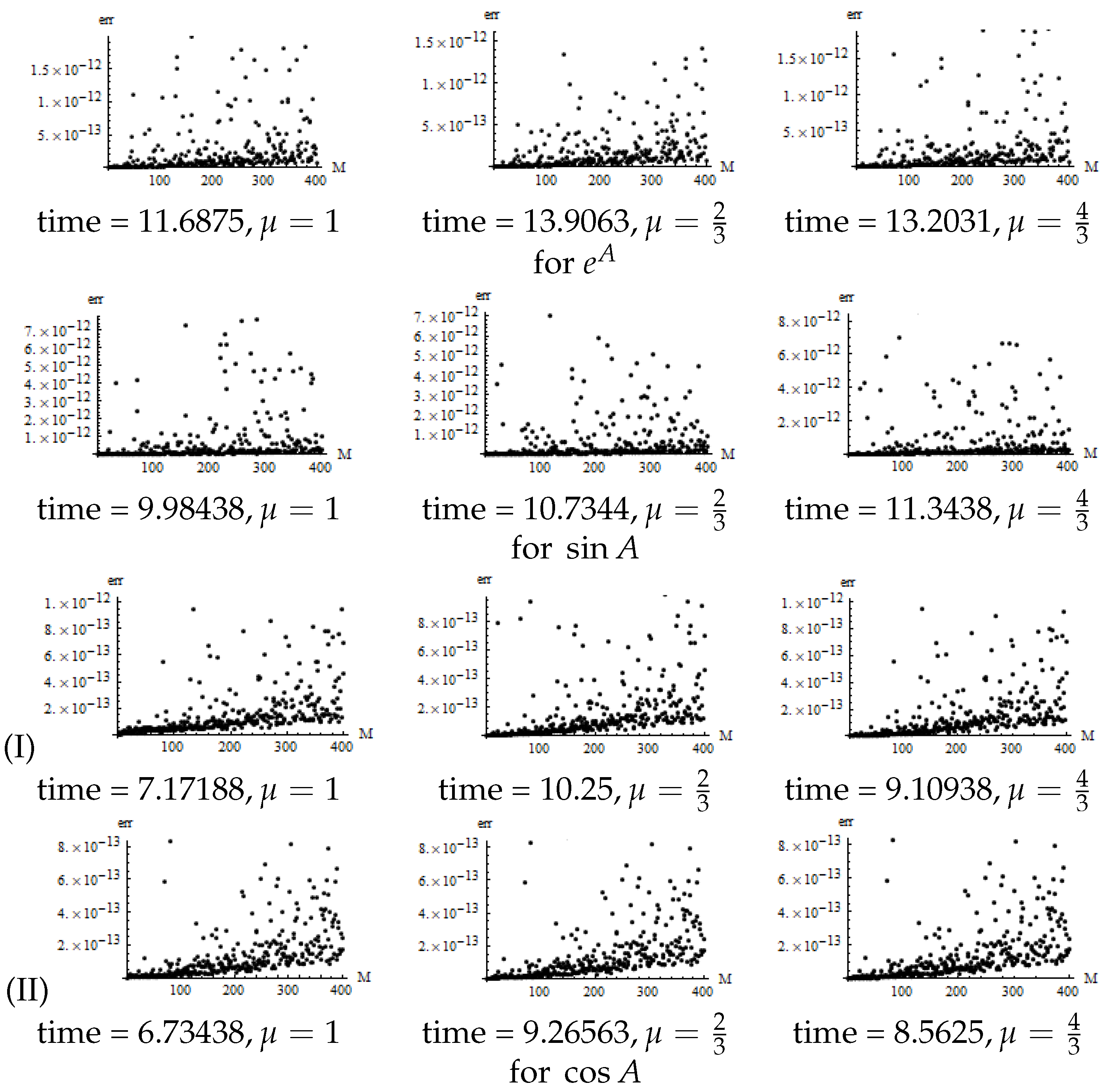
Let $A_i(i=1,2,\cdots ,M)$ be M matrices produced by (32). From Figure 1, it is evident that the calculation accuracy is essentially the same for $\mu =1,\frac{2}{3},\frac{4}{3}$, but $\mu =1$ provides the highest efficiency. The double-angle formula is notably more efficient and accurate than the triple-angle formula for $cosA$. Henceforth, we will exclude the case that utilizes the triple-angle formula for $cosA$.

Figure 1. Error comparison of the algorithms in Table 1 for $\mu =1,\frac{2}{3},\frac{4}{3}$.

Now let us juxtapose the algorithms presented in Table 1 with the internal functions and commonly used algorithms found in mathematical software. For ease of reference, let $err\left(g\right)$ denote the calculation error of matrix function $f\left(A_i\right)(i=1,2,\cdots ,M)$, where a blank g implies the utilization of the algorithms in Table 1, Table 2 and Table 3 of this article. If $g=Sym$, $Pade$, $\cdots ,$ it signifies calculation according to the internal function, Padé approximation, $\cdots ,$ respectively. When $p=16,$ $m_p=7,4,3$ for $e^A,cosA(coshA),sinA(sinhA),$ respectively. We denote the Padé approximation of $sinx$ as $r_{66}\left(x\right)$ and the Padé approximation of $e^x$ and $cosx$ as $r_{88}\left(x\right).$ In Table 1, the Padé approximation of $e^A,cosA(coshA),sinA(sinhA)$ is as follows:

$$\begin{array}{c}{r}_{88}\left(x\right)=\frac{1+\frac{x}{2}+\frac{x^2}{60}+\frac{x^3}{60}+\frac{x^4}{624}+\frac{x^5}{9360}+\frac{x^6}{205920}+\frac{x^7}{7207200}+\frac{x^8}{518918400}}{1-\frac{x}{2}+\frac{x^2}{60}-\frac{x^3}{60}+\frac{x^4}{624}-\frac{x^5}{9360}+\frac{x^6}{205920}-\frac{x^7}{7207200}+\frac{x^8}{518918400}}\mathrm{for}{e}^x,\hfill \\ r_{88}\left(x\right)=\frac{1\mp \frac{260735x^2}{545628}+\frac{4375409x^4}{141863280}\mp \frac{7696415x^6}{1310867072}+\frac{80737373x^8}{23594700729600}}{1\pm \frac{12079x^2}{545628}+\frac{34709x^4}{141863280}\pm \frac{109247x^6}{65540835360}+\frac{11321x^8}{1814976979200}}\mathrm{for}\left\{\begin{array}{c}cosx\\ coshx\end{array}\right\},\hfill \\ r_{66}\left(x\right)=\frac{x\mp \frac{7x^3}{60}+\frac{x^5}{600}}{1\pm \frac{x^2}{20}+\frac{x^4}{600}\pm \frac{x^6}{14400}}\mathrm{for}\left\{\begin{array}{c}sinx\\ sinhx\end{array}\right\}.\hfill \end{array}$$

(34)

Table 2. The fast algorithms for $tanA,secA,tanhA$, and $sechA$.

	${\mathit{m}}_{\mathit{p}},\mathit{N}$	Algorithm
$\left\{\begin{array}{c}tanA\\ tanhA\end{array}\right\}$	$m_p=\left[\sqrt{\frac{2pln10}{ln3}}\right],N=N_1+1$	$B=\frac{A^2}{3^{2N}}$,
		$C=\frac{2A}{3^N}{\displaystyle \sum _{j=0}^m}{(\pm 1)}^j\sigma (j+1)\left(4^{j+1}-1\right)B^j$
		$for(i=0,i<N,i++)$
		$C=C(3I\mp C^2){(I\mp 3C^2)}^{-1}$
		$\left\{\begin{array}{c}tanA\\ tanhA\end{array}\right\}\approx C$
$\left\{\begin{array}{c}secA\\ sechA\end{array}\right\}$	$m_p=\left[\sqrt{\frac{2pln10}{ln3}}\right],N=N_2+1$	$B=\frac{A^2}{3^{2N}},I+{\displaystyle \sum _{j=1}^m}{(\mp 1)}^j{\widehat{E}}_j{B}^j$
		$for(i=0,i<N,i++)$
		$C=C^3{(4I-3C^2)}^{-1}$
		$\left\{\begin{array}{c}secA\\ sechA\end{array}\right\}\approx C$
$N_1=\left[\frac{pln10+ln\left(2\sigma (m_p+2)\right)}{(2m_p+3)ln3}+\frac{ln\lambda }{ln3}\right],N_2=\left[\frac{pln10+ln{\widehat{E}}_{m_p+1}}{(2m_p+3)ln3}+\frac{ln\lambda }{ln3}\right].$

Table 3. The fast algorithms for $cotA,cothA,cscA,$ and $\mathrm{csch}A$.

	${\mathit{m}}_{\mathit{p}},\mathit{N}$	Algorithm
$\left\{\begin{array}{c}cotA\\ cothA\end{array}\right\}$	$m_p=\left[\sqrt{\frac{7pln10}{5ln3}}\right],N=N_1+1$	$B=\frac{A^2}{3^{2N}},C=I-2{\displaystyle \sum _{j=1}^m}{(\pm 1)}^j\sigma \left(j\right)B^j$
		$for(i=0,i<N,i++)$
		$(C=3(C(3B\mp C^2){(B\mp 3C^2)}^{-1};B=9B)$
		$\left\{\begin{array}{c}cotA\\ cothA\end{array}\right\}\approx C$
$\left\{\begin{array}{c}cscA\\ \mathrm{csch}A\end{array}\right\}$	$m_p=\left[\sqrt{\frac{5pln10}{2ln3}}\right],N=N_2+1$	$B=\frac{A^2}{3^{2N}},I+2{\displaystyle \sum _{j=1}^{m+1}}{(\pm 1)}^j\sigma \left(j\right)\left(1-\frac{2}{4^j}\right)B^j$
		$for(i=0,i<N,i++)$
		$(C=3C^3{(3C^2\mp 4B)}^{-1};B=9B)$
		$\left\{\begin{array}{c}cscA\\ \mathrm{csch}A\end{array}\right\}\approx C$
$N_1=\left[\frac{pln10+ln\left(2\sigma (m_p+2)\right)}{(2m_p+3)ln3}+\frac{ln\lambda }{ln3}\right],N_2=\left[\frac{pln10+ln{\widehat{E}}_{m_p+1}}{(2m_p+3)ln3}+\frac{ln\lambda }{ln3}\right]$

For the algorithms in Table 1, the $err\left(g\right)\left(A\right)$ of random matrix from order 1 to 800 is as follows.

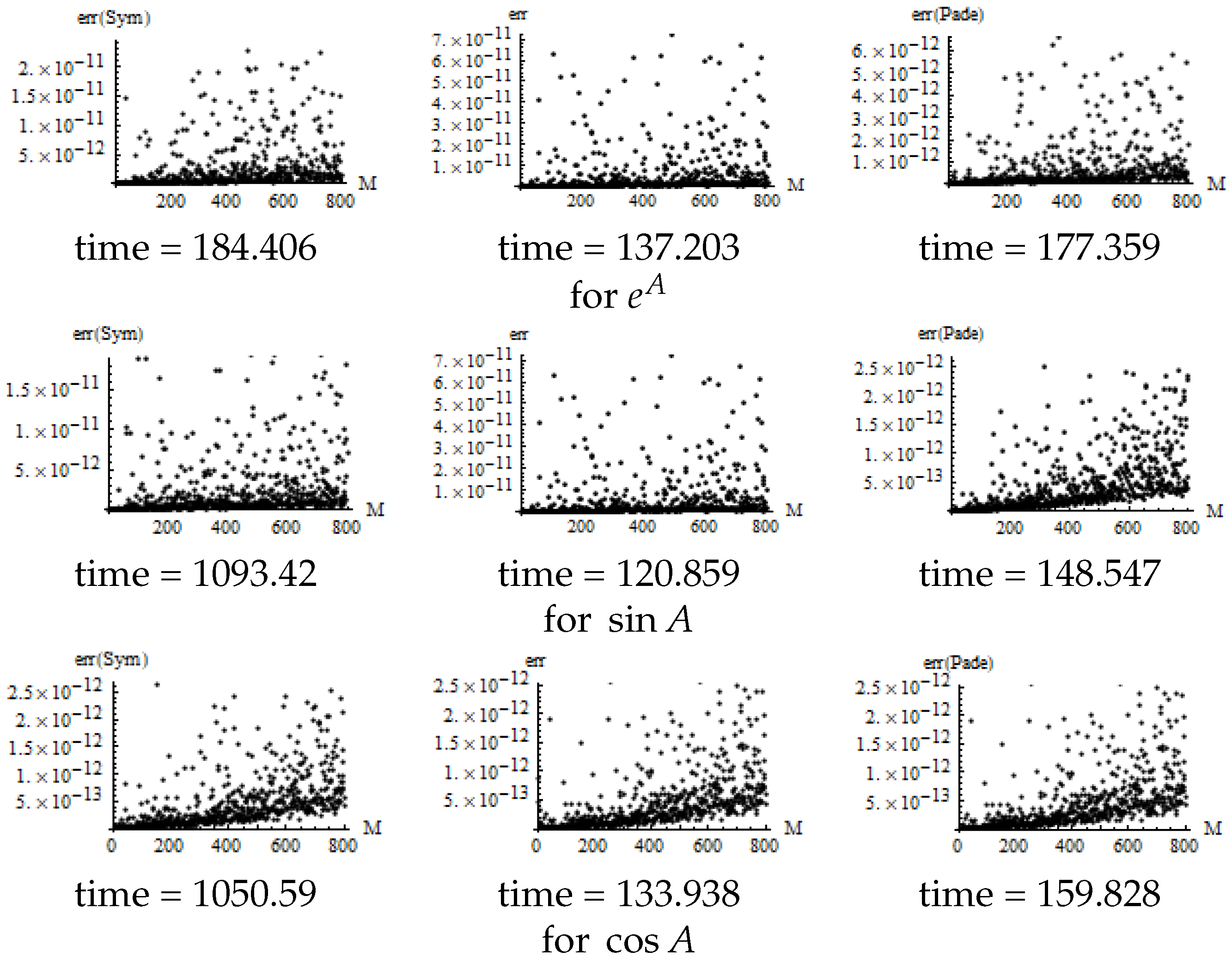
It is evident from Figure 2 that, for $e^A,cosA,$ and $sinA$, the accuracy obtained by the three methods is essentially the same. However, when the matrix order is relatively high, the Taylor expansion method presented in Table 1 outperforms the others. In particular, for cos and $sinA$, the calculation time of the internal functions is approximately eight times longer than that of the algorithms in Table 1. Numerical calculations demonstrate that while the calculation speed of $cosA$ and $sinA$ using the internal functions $Re\left(e^{iA}\right)=cosA$ and $Im\left(e^{iA}\right)=sinA$ is faster than that of the internal functions $cosA$ and $sinA$, their calculation accuracy is relatively poor.

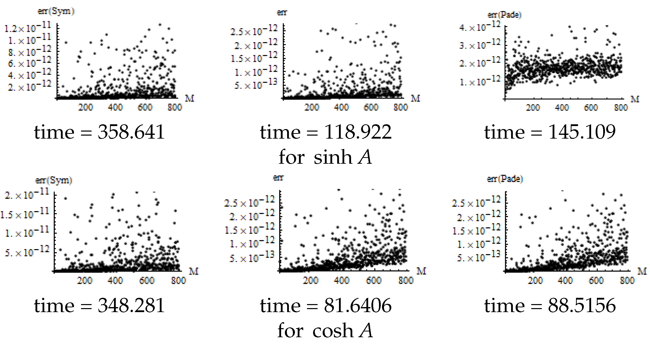
Figure 2. Error of $e^A,cosA,\mathrm{and}sinA$ for three algorithms.

For $coshA$ and $sinhA$, the internal functions can be calculated by utilizing the following equation:

$$\begin{array}{c}coshA=\frac{1}{2}(e^A+e^{-A}),sinhA=\frac{1}{2}(e^A-e^{-A}).\end{array}$$

(35)

Our experiment provides the following results for $err\left(g\right)\left(A\right)$ of random matrices with orders from 1 to $800.$

It is evident from Figure 3 that using (35) not only doubles the calculation time but also makes the calculation error substantial. Furthermore, by observing Figure 2 and Figure 3, it becomes apparent that the algorithms in Table 1 outperform the Padé approximation algorithm.

Figure 3. Error of $sinhA \mathrm{and} coshA$ for three algorithms.

4. Fast Algorithm for $\mathbf{tan}\mathit{A},\mathbf{tanh}\mathit{A},\mathbf{sec}\mathit{A}$, and $\mathit{sechA}$

Now let us contemplate the swift computation of $tanA,tanhA$, $secA$, and $sechA$. Although these matrix functions can be computed using the following approach, we aim to directly compute them, as demonstrated in the previous section.

$$\begin{array}{c}tanA=sinA{(cosA)}^{-1},secA={(cosA)}^{-1},\hfill \\ tanhA=sinhA{(coshA)}^{-1}=\left(e^A-e^{-A}\right){\left(e^A+e^{-A}\right)}^{-1},\hfill \\ sechA={(coshA)}^{-1}=2{\left(e^A+e^{-A}\right)}^{-1}.\hfill \end{array}$$

(36)

While the Padé approximation significantly contributes to matrix function computation, the numerical results in the previous section indicate that, based on the algorithm presented in this paper, neither the calculation accuracy nor the calculation speed is predominant. Therefore, this section does not adopt it.

Theorem  3.

For $tanA,secA,tanhA$, and $sechA,$ we have the following fast algorithm based on Theorem 1.

In Table 2, for $\sigma \left(j\right)$ and ${\widehat{E}}_j$, we have the following recursive formula [1]:

$$\begin{array}{c}\sigma \left(2n\right)=\frac{4}{4n+1}{\displaystyle \sum _{l=1}^{n-1}}{\sigma \left(l\right)\sigma (2n-l)+\frac{2}{4n+1}\sigma }^2\left(n\right),n=1,2,\cdots ,\hfill \\ \sigma \left(2n-1\right)=\frac{4}{4n-1}{\displaystyle \sum _{l=1}^{n-1}}\sigma \left(l\right)\sigma (2n-1-l),n=2,3,\cdots \hfill \\ {\widehat{E}}_n=-{\displaystyle \sum _{k=0}^{n-1}}\frac{{\widehat{E}}_k}{(2n-2k)!},{\widehat{E}}_0=1,\sigma \left(1\right)=\frac{1}{6}.\hfill \end{array}$$

(37)

Using the algorithms in Table 2, our experiments generated the following data for the $err\left(g\right)\left(A\right)$ of random matrices from order 1 to 200.

Here, $Sym$ indicates that matrix functions $tanA$, $tanhA$, $secA$, and sech$A,$ expressed by $sinA{\left(cosA\right)}^{-1}$, $e^A-e^{-A}{\left(e^A+e^{-A}\right)}^{-1}$, ${\left(cosA\right)}^{-1}$ and $2{\left(e^A+e^{-A}\right)}^{-1},$ respectively, are computed using the internal functions. As observed in Figure 4, the algorithm’s computation speed in Table 2 surpasses that of the internal function, particularly for $tanA$ and $secA$, where the speed is increased by 8–11 times compared to the internal function, while maintaining consistent accuracy is consistent. When the order n of the matrix is relatively large, for $tanhA$ and $sechA,$ the calculation speed is twice that of the internal function, yet the precision remains the same as the internal function.

Figure 4. Error of the $tanA,secA,tanhA,\mathrm{and}sechA$ for two algorithms.

Let us consider implementing our algorithms for calculating the functions $cotA,cotA$, $cscA$, and cschA. By

$$\begin{array}{c}cot\left(At\right)\approx A^{-1}-2{\displaystyle \sum _{j=0}^m}\sigma (j+1)A^{2j+1};(o<\left|A\right|<\pi ,z\ne 0),\hfill \\ \coth \left(At\right)\approx A^{-1}+2{\displaystyle \sum _{j=0}^m}{(-1)}^j\sigma (j+1)A^{2j+1}(0<\left|A\right|<\pi ),\hfill \\ csc\left(At\right)\approx A^{-1}+2{\displaystyle \sum _{j=0}^m}\sigma (j+1)\left(1-\frac{2}{4^{j+1}}\right)A^{2j+1}(0<\left|A\right|<\pi ),\hfill \\ \mathrm{csch}\left(At\right)\approx A^{-1}-2{\displaystyle \sum _{j=0}^m}{(-1)}^j\sigma (j+1)\left(1-\frac{2}{4^{j+1}}\right)A^{2j+1}(0<\left|A\right|<\pi ),\hfill \end{array}$$

(38)

we see that when $∥A∥$ is small, the norm of the inverse of A will be large, so the calculation using (38) will produce large errors. Therefore, we must utilize the following method:

$$\begin{array}{c}cotA=A^{-1}{cot}_{1}A,cothA=A^{-1}{coth}_{1}A,\hfill \\ cscA=A^{-1}{csc}_{1}A,\mathrm{csch}A=A^{-1}{\mathrm{csch}}_{1}A,\hfill \end{array}$$

(39)

where

$$\begin{array}{c}{cot}_{1}A\approx I-2{\displaystyle \sum _{j=1}^{m+1}}\sigma \left(j\right)A^{2j};(\left|z\right|<\pi ,z\ne 0),\hfill \\ {\coth }_{1}A\approx I-2{\displaystyle \sum _{j=1}^{m+1}}{(-1)}^j\sigma \left(j\right)A^{2j}(\left|z\right|<\pi ,z\ne 0),\hfill \\ {csc}_{1}A\approx I+2{\displaystyle \sum _{j=1}^{m+1}}\sigma \left(j\right)\left(1-\frac{2}{4^j}\right)A^{2j}(\left|z\right|<\pi ,z\ne 0),\hfill \\ {\mathrm{csch}}_{1}A\approx I+2{\displaystyle \sum _{j=1}^{m+1}}{(-1)}^j\sigma \left(j\right)\left(1-\frac{2}{4^j}\right)A^{2j}(\left|z\right|<\pi ,z\ne 0).\hfill \end{array}$$

(40)

Theorem  4.

Using Theorem 1, we have the following algorithm for $cotA,cothA,cscA,$ and $sechA$.

Implementation of the algorithms in Table 3 provides the following results for the matrix functions in (39).

Here, $Sym$ signifies that matrix functions $cotA$, $cothA$, $cscA$, and $sechA$ are calculated using the internal functions with the regular formulas $cosA{\left(sinA\right)}^{-1}$, $\left(e^A+e^{-A}\right){\left(e^A-e^{-A}\right)}^{-1}$, ${\left(sinA\right)}^{-1}$, and $2{\left(e^A-e^{-A}\right)}^{-1},$ respectively. The results in Figure 5 are essentially consistent with the corresponding results in Figure 2.

Figure 5. Error of $cotA,cotA,cscA,\mathrm{and}cschAfortwoalgorithms$.

5. Fast Algorithm for Logarithmic Matrix Function $ln\mathit{A}$ and Some Related Functions

People consider various algorithms [17,18,19,20,21,22] for logarithmic matrix function $lnA.$ One of the most effective methods we noticed was the following algorithm. The standard way of dealing with this problem is to use the square root operator repeatedly to bring A near the identity:

$$\begin{array}{c}lnA=2^{k}ln{A}_k,A_k=A^{1/2^k}.\hfill \end{array}$$

(41)

As k increases, $A^{1/2^k}$$\to I$, so for sufficiently large k, we can apply a direct method to $A^{1/2^k}.$ This procedure for the logarithm was introduced by Kenney and Laub [19]. The specific method is to choose k such that

$$\begin{array}{c}∥A^{1/2^k}-I∥<\alpha <1,\hfill \end{array}$$

(42)

and usually, k is selected from 8. We slightly optimize the method as follows:

$$\begin{array}{c}lnA=ln\lambda ·I+2^{k}ln{A}_k,A_k=A_0^{1/2^k},A_0=\frac{1}{∥A∥}A,\hfill \end{array}$$

(43)

and

$$\begin{array}{c}∥A_0^{1/2^k}-I∥<\alpha <1,\hfill \end{array}$$

(44)

where k is usually selected from 4.

For $lnx$, the algorithm that converges faster is

$$\begin{array}{c}lnx=ln\frac{1-y}{1+y}\approx -2{\displaystyle \sum _{j=1}^m}\frac{y^{2j+1}}{2j+1},\hfill \end{array}$$

(45)

where $y=\frac{1-x}{1+x}.$ For $ln{A}_k$, we have

$$\begin{array}{c}ln{A}_k=ln\left(I-B\right)-ln\left(I+B\right)\approx -2{\displaystyle \sum _{j=1}^m}\frac{B^{2j}}{2j+1},\hfill \end{array}$$

(46)

where $B=(I-A_k){(I+A_k)}^{-1}.$ Applying the Euler–Abel transformation [21], we obtain the following accelerated series:

$$\begin{array}{c}ln{A}_k\approx \frac{1}{3}B{F}^2(I-12{\displaystyle \sum _{j=1}^m}\frac{B^{2j}}{(2j+3)(4j^2-1)})-F,\hfill \end{array}$$

(47)

where $F=2B{(I-B^2)}^{-2}.$ We can use the following Padé approximation of $ln{A}_k$ [20].

$$\begin{array}{c}ln{A}_k\approx (B+2B^2+\frac{47}{36}{B}^3+\frac{11}{36}{B}^4+\frac{137}{7560}{B}^5)F,\hfill \\ F={(I+\frac{5}{2}B+\frac{20}{9}{B}^2+\frac{5}{6}{B}^3+\frac{5}{42}{B}^4+\frac{1}{252}{B}^5)}^{-1},\hfill \end{array}$$

(48)

where $B=A_k-I.$ We also provide some numerical results for the matrix function $lnA.$

Based on (41)–(44) we also provide some numerical results of $lnA$ using (46)–(48). It can be seen from Figure 6 that through optimization (43), the calculation accuracy of (46)–(48) is significantly improved, and the calculation speed of (46)–(48) is more than twice as fast as the inner function. The calculation speed advantage of the Padé approximation is obvious.

Figure 6. Error of $lnA$ for the several algorithms.

We used the following identities to implement our general algorithm for the computations of the inverse trigonometric and hyperbolic functions. To control the length of the paper, we will not display the results here.

$$\begin{array}{c}arcsinx=2arcsin\frac{x}{\sqrt{2(1+\sqrt{1-x^2})}},\hfill \\ arctanx=2arctan\frac{x}{1+\sqrt{1+x^2}},\hfill \\ arcsinx=x+{\displaystyle {\displaystyle \sum _{l=1}^{\infty }}}\frac{(2l-1)x^{2l+1}}{\left(2l\right)!(2l+1)},arctanx={\displaystyle {\displaystyle \sum _{l=0}^{\infty }}}\frac{x^{2l+1}}{(2l+1)},\hfill \end{array}$$

(49)

$$\begin{array}{c}\mathrm{arcsinh}x=2\mathrm{arcsinh}\frac{x}{\sqrt{2(1+\sqrt{1+x^2)}}},\mathrm{arctanh}x=2\mathrm{arctanh}\frac{x}{1+\sqrt{1-x^2}},\hfill \\ \mathrm{arcsinh}x=x+{\displaystyle {\displaystyle \sum _{l=1}^{\infty }}}\frac{{(-1)}^l(2l-1)x^{2l+1}}{\left(2l\right)!(2l+1)},arctanhx={\displaystyle \sum _{l=0}^{\infty }}\frac{{(-1)}^l{x}^{2l+1}}{(2l+1)}.\hfill \end{array}$$

(50)

For $arcsinA,arctanA,$ arcsinh$A,\mathrm{and}$ arctanh$A,$ under certain conditions, we can use the following identity.

$$\begin{array}{c}arcsinA=-iln\left(\sqrt{I-A^2}+iA\right),\mathrm{arcsinh}A=ln\left(\sqrt{I+A^2}+A\right),\hfill \\ arctanA=\frac{i}{2}ln\left(\left(iI+A\right){\left(iI-A\right)}^{-1}\right),\hfill \\ \mathrm{arctanh}A=\frac{1}{2}ln\left((I+A){(I-A)}^{-1}\right).\hfill \end{array}$$

(51)

6. Improved Calculation Formula for Initial Value Problems (3) and (8)

Now, let us consider the calculation of the integral in (11), i.e.,

$$\begin{array}{c}{\widehat{F}}_k={\int }_0^{\tau }{e}^{Hs}{F}_H(k\tau -s)ds.\end{array}$$

(52)

If numerical integration is used to calculate this integral, it is quite time-consuming, and the calculation accuracy cannot be guaranteed. We adopt the following method here. For $nn=1,2,\cdots$, there is the following relationship:

$$\begin{array}{c}{\widehat{F}}_k={\displaystyle {\displaystyle \sum _{j=0}^{nn-1}}}{\int }_{\frac{j\tau }{nn}}^{\frac{j\tau }{nn}}{e}^{Hs}{F}_H(k\tau -s)ds={\displaystyle {\displaystyle \sum _{j=0}^{nn-1}}}{T}_{nn,j}{\int }_0^{\frac{\tau }{nn}}{e}^{Hs}{F}_H(k\tau -\frac{j\tau }{nn}-s)ds\\ \approx {\displaystyle {\displaystyle \sum _{j=0}^{nn-1}}}{T}_{nn,j}{\displaystyle {\displaystyle \sum _{l=0}^m}}\frac{H^l}{l!}{\int }_0^{\frac{\tau }{nn}}{s}^l{F}_H(k\tau -\frac{j\tau }{nn}-s)ds,\end{array}$$

(53)

where

$$\begin{array}{c}{T}_{nn,0}=I,T_{nn}=e^{H\frac{\tau }{nn}},T_{nn,j}=e^{H\frac{j\tau }{nn}}=T_{nn}{T}_{nn,j-1},j=1,2,\cdots ,nn-1.\end{array}$$

(54)

$T_{nn}$ can be calculated by the following method:

$$\begin{array}{c}{T}_{nn}=I,zz=I;\hfill \\ \mathrm{for}(i=1,i\le m,i++)(zz=\frac{\frac{\tau }{nn}}{i}H\times zz;T_{nn}=T_{nn}+zz).\hfill \end{array}$$

(55)

So, (53) can be written as follows:

$$\begin{array}{c}{\widehat{F}}_k\approx {\displaystyle \sum _{j=0}^{nn-1}}{T}_{nn,j}{H}_j,H_j={\displaystyle \sum _{l=0}^m}\frac{H^l}{l!}{\int }_0^{\frac{\tau }{nn}}{s}^l{F}_H(k\tau -\frac{j\tau }{nn}-s)ds,\end{array}$$

(56)

so we can convert the integral of the product of matrix exponential function and vector function into the integral of pure vector function.

The improved calculation formula for (3) is as follows:

$$\begin{array}{c}\left(55\right),\left(56\right),\hfill \\ U_k=T{U}_{k-1}+{\displaystyle \sum _{j=0}^{nn-1}}{T}_{nn,j}{H}_j,k=1,2,\cdots ,\hfill \end{array}$$

(57)

where $T=e^{H\tau }$ is calculated by the algorithm in Table 1, and $T_{nn,j}and{H}_j$ are calculated by (55) and (56).

For

$$\begin{array}{c}{\int }_0^{\frac{\tau }{nn}}{s}^l{F}_H(k\tau -\frac{j\tau }{nn}-s)ds,\hfill \end{array}$$

(58)

the following two algorithms can be used.

(1) Integrable function method If $F\left(t\right)={(f_1\left(t\right),f_2\left(t\right),\cdots ,f_v\left(t\right),\cdots ,f_n\left(t\right))}^T,$ $f_v\left(t\right)$ is the algebraic sum of functions of the following types:

$$\begin{array}{c}{t}^{\alpha },t^l{e}^{-\omega t},t^{l}sin\omega t,t^{l}cos\omega t,\hfill \end{array}$$

(59)

then (58) can be expressed in analytical form, so $H_j$ can also be expressed in analytical form. In this way, the calculation of (57) can be completed.

(2) Gauss three-point integral formula

Note that, under 16-bit calculation accuracy,

$$\begin{array}{c}\frac{\tau }{nn}<\frac{1}{2^{n_{16}}{\lambda }_H}\approx \frac{0.0376434}{\left|{\lambda }_H\right|}<0.0376434,\hfill \end{array}$$

(60)

and the algebraic accuracy of the Gauss three-point integral formula is 5. Using the Gauss three-point integral formula,

$$\begin{array}{c}\frac{1}{2}{\left(\frac{\tau }{nn}\right)}^{l+1}{\sum }_{i=1}^3{w}_i{\left(\frac{1+b_i}{2}\right)}^l{F}_H(k\tau -\frac{(j+1/2)\tau }{nn}-\frac{b_i\tau }{2nn}),\hfill \end{array}$$

(61)

where $w_1=w_3=\frac{5}{9},w_2=\frac{8}{9},b_1=-\frac{\sqrt{15}}{5},b_2=0,b_3=\frac{\sqrt{15}}{5},$ to approximate (58) with high accuracy. So, (57) can be replaced by the following algorithm.

Algorithm  1.

Numerical solution algorithm of initial value problem (3): for $nn=1,2,\cdots$

$$\begin{array}{c}{U}_k=T{U}_{k-1}+\frac{\tau }{2nn}{\displaystyle \sum _{j=0}^{nn-1}}{T}_{nn,j}\sum _{i=1}^3{w}_i{e}^{H\frac{(1+b_i)\tau }{2nn}}{F}_H\left(k\tau -\frac{(2j+1+b_i)\tau }{2nn}\right),k=1,2,\cdots ,\hfill \end{array}$$

(62)

where

$$\begin{array}{c}{e}^{H\frac{(1+b_i)\tau }{2nn}}\approx \frac{w_i\tau }{2nn}\left(I+{\displaystyle \sum _{l=1}^m}\frac{1}{l!}{\left(\frac{(1+b_i)\tau }{2nn}\right)}^l{H}^l\right).\hfill \end{array}$$

(63)

In particular, if we let

$$\begin{array}{c}nn=\left\{\begin{array}{c}\left[2^{n_p}{\lambda }_H\tau \right]+12^{n_p}{\lambda }_H\tau >1\\ 12^{n_p}{\lambda }_H\tau \le 1\end{array}\right.,\hfill \end{array}$$

(64)

then $N_p=0,m=m_p=\left[\sqrt{\frac{9pln10}{8ln2}}\right],$

$$\begin{array}{c}{W}_{i,H}\approx \frac{w_i\tau }{2nn}\left(I+{\displaystyle \sum _{l=1}^{m_p}}\frac{1}{l!}{\left(\frac{(1+b_i)\tau }{2nn}\right)}^l{H}^l\right).\hfill \end{array}$$

(65)

At this time, the theoretical calculation accuracy of (62) is $p.$

Remark  3.

Note that, $W_{i,H}(i=1,2,3)$ in (63) and (65) only needs to be calculated once, and is independent of $F\left(t\right)$, which is not only efficient but also easy to program.

Now let us consider the numerical solution of the initial value problem (8). If it is converted to the initial value problem (3), then

$$\begin{array}{c}\left(\begin{array}{c}x\left(t\right)\\ x\prime \left(t\right)\end{array}\right)=U,H=\left(\begin{array}{cc}0& I_{3\times 3}\\ -K& 0\end{array}\right),F_H\left(t\right)=\left(\begin{array}{c}0\\ F\left(t\right)\end{array}\right),U_0=\left(\begin{array}{c}{x}_0\\ x_1\end{array}\right).\end{array}$$

(66)

By

$$\begin{array}{c}{W}_{i,H}=e^{\tau H}\approx \left(\begin{array}{cc}{cos}_p\left(\tau A\right)& \tau {sin}_{1,p}\left(\tau A\right)\\ -K\tau {sin}_{1,p}\left(\tau A\right)& {cos}_p\left(\tau A\right)\end{array}\right),A=\sqrt{K},\hfill \end{array}$$

(67)

where

$$\begin{array}{c}{sin}_{1}A={\displaystyle \sum _{j=0}^{\infty }}\frac{{(-1)}^j}{(2j+1)!}{A}^{2j}={\displaystyle \sum _{j=0}^{\infty }}\frac{{(-1)}^j}{(2j+1)!}{K}^j,\hfill \end{array}$$

(68)

and (68), we obtain the following algorithm.

Algorithm  2.

 

$$\begin{array}{c}\Delta t=\tau /3^N;T_{\alpha }=I;zz=I;A_2=(A\Delta t)\times (A\Delta t);\hfill \\ \mathit{for}(i=1,i\le m,i++)(zz=-\frac{A_2}{\left(2i\right)(2i+1)}\times zz;T_{\alpha }=T_{\alpha }+zz),\hfill \end{array}$$

(69)

and

$$\begin{array}{c}\mathit{for}(i=0,i<N,i++)\hfill \\ (zz=T_{\alpha }\times T_{\alpha },zz=zz\times A_2,A_2=9A_2,T_{\alpha }=T_{\alpha }-\frac{4}{3}{T}_{\alpha }\times zz),\hfill \end{array}$$

(70)

where $m_p$ and $N_p$ are determined using (31).

Algorithm  3.

Numerical solution algorithm of initial value problem (8):

$$\begin{array}{c}{x}_k=\left(cos\left(\tau A\right)x_{k-1}+\tau {sin}_1\left(\tau A\right)y_{k-1}\right)\hfill \\ +\frac{\tau }{2nn}{\displaystyle \sum _{j=0}^{nn-1}}{\sum }_{i=1}^3\frac{w_i(2j+1+b_i)\tau }{2nn}{sin}_1\left(\frac{(2j+1+b_i)\tau }{2nn}A\right)F(k\tau -\frac{(2j+1+b_i)\tau }{2nn})\hfill \\ y_k=-Asin\left(\tau A\right)x_{k-1}+cos\left(\tau A\right)y_{k-1}\hfill \\ +\frac{\tau }{2nn}{\displaystyle \sum _{j=0}^{nn-1}}{\sum }_{i=1}^3{w}_{i}cos\left(\frac{(2j+1+b_i)\tau }{2nn}A\right)F(k\tau -\frac{(2j+1+b_i)\tau }{2nn})\hfill \end{array}$$

(71)

for $nn=1,2,\cdots ,$ where $A=\sqrt{K}.$ In particular, if $nn$ is determined using (64), the theoretical accuracy of this algorithm is p and

$$\begin{array}{c}{x}_k=cos\left(\tau A\right)x_{k-1}+\tau {sin}_1\left(\tau A\right)y_{k-1}+\frac{\tau }{2nn}{\displaystyle \sum _{j=0}^{nn-1}}{\displaystyle \sum _{i=1}^3}{w}_{i}T{W}_{j,i}^{sin}F(k\tau -\frac{(2j+1+b_i)\tau }{2nn}),\hfill \\ y_k=cos\left(\tau A\right)y_{k-1}-Asin\left(\tau A\right)x_{k-1}+\frac{\tau }{2nn}{\displaystyle \sum _{j=0}^{nn-1}}{\displaystyle \sum _{i=1}^3}{w}_{i}T{W}_{j,i}^{cos}F(k\tau -\frac{(2j+1+b_i)\tau }{2nn}),\hfill \\ x_0=x\left(0\right),y_0=x\prime \left(0\right),\hfill \end{array}$$

(72)

where

$$\begin{array}{c}T{W}_{j,i}^{sin}=\frac{(1+b_i)\tau }{2nn}cos\left(\frac{j\tau }{nn}A\right){sin}_{1,m_p}\left(\frac{(1+b_i)\tau }{2nn}A\right)\hfill \\ +\frac{j\tau }{nn}{sin}_1\left(\frac{j\tau }{nn}A\right){cos}_{m_p}\left(\frac{(1+b_i)\tau }{2nn}A\right),\hfill \\ T{W}_{j,i}^{cos}=cos\left(\frac{j\tau }{nn}A\right){cos}_{m_p}\left(\frac{(1+b_i)\tau }{2nn}A\right)\hfill \\ -sin\left(\frac{j\tau }{nn}A\right){sin}_{m_p}\left(\frac{(1+b_i)\tau }{2nn}A\right),\hfill \end{array}$$

(73)

and

$$\begin{array}{c}{sin}_{m_p}\left(sA\right)=A{\displaystyle \sum _{l=0}^{m_p}}\frac{{(-1)}^l{s}^{2l+1}{K}^l}{(2l+1)!},\hfill \\ {sin}_{1,m_p}\left(sA\right)={\displaystyle \sum _{l=0}^{m_p}}\frac{{(-1)}^l{s}^{2l}{K}^l}{(2l+1)!},\hfill \\ {cos}_{m_p}\left(sA\right)=I+{\displaystyle \sum _{l=1}^{m_p+1}}\frac{{(-1)}^l{s}^{2l}{K}^l}{\left(2l\right)!}.\hfill \end{array}$$

(74)

If A is reversible, then

$$\begin{array}{c}{x}_k=cos\left(\tau A\right)x_{k-1}+A^{-1}sin\left(\tau A\right)y_{k-1}\hfill \\ +\frac{\tau }{2nn}{A}^{-1}{\displaystyle \sum _{j=0}^{nn-1}}\sum _{i=1}^3{w}_{i}sin\left(\frac{(2j+1+b_i)\tau }{2nn}A\right)F(k\tau -\frac{(2j+1+b_i)\tau }{2nn})\hfill \\ y_k=-Asin\left(\tau A\right)x_{k-1}+cos\left(\tau A\right)y_{k-1}\hfill \\ +\frac{\tau }{2nn}{\displaystyle \sum _{j=0}^{nn-1}}\sum _{i=1}^3{w}_{i}cos\left(\frac{(2j+1+b_i)\tau }{2nn}A\right)F(k\tau -\frac{(2j+1+b_i)\tau }{2nn}).\hfill \end{array}$$

(75)

Therefore, (75) can be written in the form of complex function as follows:

$$\begin{array}{c}{z}_k=e^{-i\tau A}{z}_{k-1}+\frac{i\tau }{2nn}{A}^{-1}{\displaystyle \sum _{j=0}^{nn-1}}{e}^{-\frac{j\tau i}{nn}A}\sum _{l=1}^3{w}_l{e}^{-\frac{(1+b_l)\tau i}{2nn}A}F\left(k\tau -\frac{(2j+1+b_l)\tau }{2nn}\right),\end{array}$$

(76)

or

$$\begin{array}{c}{Z}_k=e^{-i\tau A}{Z}_{k-1}+\frac{\tau }{2nn}{\displaystyle \sum _{j=0}^{nn-1}}{e}^{-\frac{j\tau i}{nn}A}\sum _{l=1}^3{w}_l{e}^{-\frac{(1+b_l)\tau i}{2nn}A}F\left(k\tau -\frac{(2j+1+b_l)\tau }{2nn}\right),\end{array}$$

(77)

where $i=\sqrt{-1},$

$$\begin{array}{c}{z}_k=x_k+i{A}^{-1}{y}_k,x_k=Re{z}_k,y_k=AIm{z}_k,\hfill \\ Z_k=y_k-iA{x}_k,y_k=Re{Z}_k,x_k=-A^{-1}Im{Z}_k.\hfill \end{array}$$

(78)

We first provide an examples to illustrate the effectiveness of Algorithms 1. Although we skip examples of Algorithm 2, we then include an example for the effectiveness of Algorithm 3.

Example  1.

In (8), let

$$\begin{array}{c}K=\left(\begin{array}{cc}1& -1\\ -1& \frac{5}{2}\\ & 1& 4\end{array}\right),F\left(t\right)=\left(\begin{array}{c}sint\hfill \\ \frac{1}{2}sint\hfill \\ cos\frac{\sqrt{2}t}{2}-cos\left(\sqrt{3}t\right)+sint\hfill \end{array}\right),\\ x_0={\left(\begin{array}{ccc}\frac{5}{2}& 0& -2\end{array}\right)}^T,x_1={\left(\begin{array}{ccc}1& 1& 2\end{array}\right)}^T.\end{array}$$

(79)

The analytic solution of the initial value problem (8) is

$$\begin{array}{c}x\left(t\right)=\left(\begin{array}{c}2cos\frac{\sqrt{2}t}{2}+\frac{1}{2}cos\left(\sqrt{3}t\right)+sint\hfill \\ cos\frac{\sqrt{2}t}{2}-cos\left(\sqrt{3}t\right)+sint\hfill \\ sin\left(2t\right)-2cos\left(2t\right)\hfill \end{array}\right).\end{array}$$

(80)

Let $er{r}_{i,k}={∥x\left(k\tau \right)-x_{i,k}∥}_{\infty }i=1,2,$ where $x_{1,k},x_{2,k}(k=0,1,2,\cdots ,N)$ are the numerical solutions of the initial value problem (8) determined by Algorithm 1 and Algorithm 3, respectively. 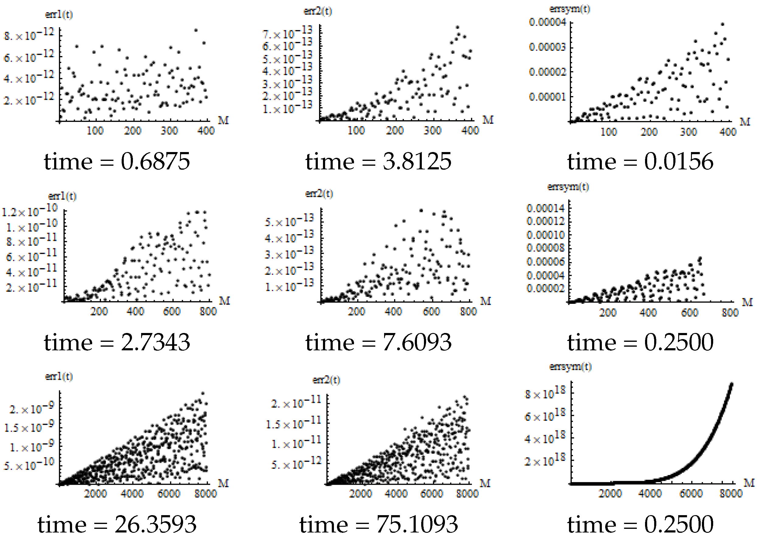$er{r}_{sym,k}={∥x\left(k\tau \right)-x_{sym}\left(k\tau \right)∥}_{\infty },$ where $x_{sym}\left(t\right)$ is the numerical solution obtained by calling the function $NDSolve$ in Mathematica. The numerical results of $er{r}_{1,k},er{r}_{2,k},er{r}_{sym,k}[0,T]$$(k=0,1,2,\cdots ,N\tau =T)$ are as follows.

It can be seen from Figure 7 that the calculation accuracy of Algorithm 1 is higher than that of Algorithm 3 but the calculation speed of Algorithm 3 is three times that of Algorithm 1. However, the error of numerical results of Mathematica internal functions is far greater than the error of Algorithms 1 and 3. In particular, the collapse is calculated at $t=667.787$. After this point, the error increases exponentially with time t. However, Algorithms 1 and 3 are quite stable. For example, the calculation error in $[0,8000]$ is still very small.

Figure 7. Error of numerical solution (8) for several algorithms ($nm$ is calculated according to (64)).

In Algorithms 1 and 3, let $nn=\mu n{n}_A,\mu =0.5,0.25,0.125$, where $n{n}_A$ is calculated according to (64). The numerical results are as follows.

Compared with Figure 7 and Figure 8, when $\mu =0.5$, the calculation accuracy is not reduced by much, and the calculation speed is almost doubled. For $\mu =0.125$ Algorithms 1 and 3, the calculation accuracy is still high, and the calculation speed is 10 times higher than that in Figure 8.

Figure 8. Error of numerical solution (8) for several algorithms.

Example  2.

In (8), let $K={\left(k_{i,j}\right)}_{n\times n}$ be a tridiagonal matrix. $F\left(t\right)={(f_1\left(t\right),f_2\left(t\right),\cdots ,f_n\left(t\right))}^T$, $f_i\left(t\right)=A_{i}cos({\omega }_{i}t+{\phi }_i)(i=1,2,\cdots ,n)$, $x_0={\left(x_{0,1},x_{0,2},\cdots ,x_{0,n}\right)}^T$, $x_1={\left(x_{1,1},x_{1,2},\cdots ,x_{1,n}\right)}^T$, and they are randomly generated and satisfy the following conditions:

$$\begin{array}{c}\left|k_{i,i}-9\right|\le 1,\left|k_{i,i+1}-\frac{3}{2}\right|\le \frac{1}{2},\left|k_{i+1,i}-\frac{3}{2}\right|\le \frac{1}{2},\\ \left|A_i-\frac{3}{2}\right|\le \frac{1}{2},\left|{\omega }_i-\frac{5}{2}\right|\le \frac{1}{2},0\le {\phi }_i\le \frac{\pi }{2},\\ \left|x_{0,i}\right|\le 1,\left|x_{1,i}\right|\le 1(i=1,2,\cdots ,n).\end{array}$$

For $n=50,100,200,\mathrm{and}400,$ the following numerical results are provided by Algorithms 1 and 3.

In Figure 9, (1)–(4), the left is the first two components of the numerical solution, and the right is the difference between the numerical solutions obtained by the two algorithms. It is noted that sometimes ${\omega }_i(i=1,2,\cdots ,n)$ is close to the frequency of the solution, and flutter or resonance may occur. However, the values obtained by the two algorithms are still very close.

Figure 9. Numerical solutions and errors of two algorithms.

7. Conclusions

In this paper, we established algorithms for the computation of matrix exponential functions, matrix trigonometric functions, and matrix hyperbolic functions. Our numerical results show that these algorithms are faster with higher accuracy compared to existing algorithms and the system algorithms in Mathematica. In the series expansion of matrix function, the number of expanded items $m_p$ is only related to the requirement of calculation accuracy, and has nothing to do with the matrix itself. However, the number of times in the iterative process $N_p$ is not only related to the matrix itself but also closely related to $t.$ When $\left|3^{n_p}{\lambda }_{A}t\right|\le 1$($\left|2^{n_p}{\lambda }_{A}t\right|\le 1$), $N_p=0$, the calculation of the matrix function becomes an algebraic operation, so the integral in (9)–(12) becomes an easy integral to compute. In brief, our algorithm allows users to set a required level of accuracy and then use it to choose appropriate values for parameters m and N to minimize computation time. In this manner, both accuracy and efficiency are addressed simultaneously.