sBERT: Parameter-Efficient Transformer-Based Deep Learning Model for Scientific Literature Classification

Abstract

This paper introduces a parameter-efficient transformer-based model designed for scientific literature classification. By optimizing the transformer architecture, the proposed model significantly reduces memory usage, training time, inference time, and the carbon footprint associated with large language models. The proposed approach is evaluated against various deep learning models and demonstrates superior performance in classifying scientific literature. Comprehensive experiments conducted on datasets from Web of Science, ArXiv, Nature, Springer, and Wiley reveal that the proposed model’s multi-headed attention mechanism and enhanced embeddings contribute to its high accuracy and efficiency, making it a robust solution for text classification tasks.

1. Introduction

The scientific community has witnessed an unprecedented surge in the volume of published literature, with millions of articles disseminated annually across myriad platforms. As of recent estimates, over 2.5 million scientific articles are published each year across more than 30,000 peer-reviewed journals globally [1,2]. In addition to journal articles, the proliferation of scientific conferences contributes significantly to the literature pool, with thousands of conferences generating substantial numbers of proceedings and papers annually. The academic sector also plays a crucial role, with universities around the world producing a vast number of theses and dissertations each year. For instance, in 2018 alone, the United States saw the publication of approximately 60,000 doctoral dissertations [3]. This exponential growth in scientific publications is facilitated by advances in digital technology and open access initiatives, further underscoring the dynamic and expansive nature of modern scientific research. The usefulness of such a large amount of information depends on how it is automatically organized and grouped into various subjects, domains, and themes. Text classification is a crucial tool for organizing, managing, and retrieving textual data repositories.

Classic machine learning-based classification algorithms have been used in the task of text classification. The problems inherent to such algorithms, such as the need for feature engineering, have limited their application. To address this, deep learning algorithms including models based on convolutional neural networks (CNN) [4,5,6,7,8] and recurrent neural networks (RNNs) [9,10] have been proposed.

Transformer-based models [11,12,13,14,15,16] have recently been used. When it comes to text categorization tasks, these models perform better than the other simpler models. However, the performance gains are accompanied by a larger and more complex model. Requiring such complex models is necessary to achieve satisfactory outcomes in sequence-to-sequence tasks. However, these models are not the best to utilize for relatively easy tasks such as text classification.

1.1. Research Questions Addressed in This Paper

• How do different text classification models compare in terms of performance for scientific literature classification (SLC)

  −

  This paper evaluates the performance of various text classification models, including CNN, RNN, and transformer-based models across multiple datasets, such as WOS, ArXiv, Nature, Springer, and Wiley.

  −

  Detailed performance metrics are provided, which highlight the strengths and weaknesses of each model.

  −

  The results indicate that sBERT (small BERT) outperforms other models in accuracy and robustness across diverse datasets.

• What are the limitations of existing CNN and RNN models in handling text classification tasks?

  −

  The Introduction (Section 1) and Related Work (Section 2) discuss the representational limitations of CNN and RNN models, particularly the challenge of detecting long-range dependencies in the input.

  −

  This sets the stage for introducing transformer-based models that address these limitations through mechanisms such as self-attention.

• How can parameter efficiency be achieved while maintaining high performance?

  −

  The proposed sBERT model is designed to utilize a multi-headed attention mechanism and hybrid embeddings to capture global context efficiently.

  −

  The paper details the architecture of sBERT, emphasizing its parameter efficiency compared to other transformer-based models.

  −

  It requires only 15.7 MB of memory and achieves rapid inference times, demonstrating a significant reduction in computational resources without compromising performance.

1.2. Paper Outline

In Section 2 of this paper, we include the relevant literature review. Section 3 introduces the proposed approach, while Section 4 provides a detailed account of the datasets employed and the experiments carried out. Section 5 is devoted to the presentation and discussion of the study’s findings.

2. Related Work

In this section, we summarize the relevant literature on various approaches to text classification. The review covers works published between 2015 and 2022 to provide a comprehensive overview of recent advances in this field.

2.1. Convolutional Neural Networks for Sentence Classification

The foundational work of Kim [4] demonstrated the effectiveness of convolutional neural networks (CNNs) for sentence classification, illustrating significant improvements in text classification tasks by employing simple yet powerful CNN architectures. Building upon this, Zhang et al. [17] introduced the Multi-Group Norm Constraint CNN (MGNC-CNN), which leveraged multiple word embeddings to enhance sentence classification performance. The utility of CNNs in combining contextual information was further explored by Wu et al. [18], who integrated self-attention mechanisms with CNNs to improve text classification accuracy.

2.2. Advances in CNN Architectures

Several studies have proposed advancements in CNN architectures for text classification. Zhang et al. [19] introduced character-level convolutional networks, highlighting their ability to handle texts at a granular level and outperforming traditional word-level models. Similarly, Conneau and Schwenk [20] developed very deep convolutional networks, emphasizing the importance of depth in CNNs for capturing intricate text patterns. Johnson and Zhang [21] compared shallow word-level CNNs and deep character-level CNNs, demonstrating that deep character-level models achieve superior performance in text categorization tasks. More recently, Wang et al. [22] combined n-gram techniques with CNNs to enhance short text classification, while Soni et al. [23] introduced TextConvoNet, a robust CNN-based architecture specifically designed for text classification.

2.3. Word Embeddings and Contextual Information

The role of word embeddings in enhancing sentence classification has been a focal point in many studies. Mandelbaum and Shalev [24] explored various word embeddings and their effectiveness in sentence classification tasks. Senarath and Thayasivam [25] further advanced this by employing multiple word-embedding models for implicit emotion classification in tweets. Additionally, the combination of recurrent neural networks (RNNs) and CNNs with attention mechanisms, as proposed by Liu et al. [9], demonstrated significant improvements in sentence representation and classification.

2.4. Hierarchical and Attention-Based Models

The introduction of hierarchical and attention-based models has significantly influenced sentence classification methodologies. Yang et al. [26] proposed Hierarchical Attention Networks (HANs), which effectively captured the hierarchical structure of documents for better classification. Zhou et al. [27] extended this approach by using attention-based LSTM networks for cross-lingual sentiment classification. Furthermore, Bahdanau et al. [28] introduced the attention mechanism in neural machine translation, which has since been widely adopted in various text classification models.

2.5. Hybrid Models and Domain-Specific Applications

Hybrid models that combine CNNs with other neural network architectures have also shown promising results. Hassan and Mahmood [29] developed a deep-learning convolutional recurrent model that took advantage of the strengths of CNN and RNN for sentence classification. In domain-specific applications, Gonçalves et al. [30] utilized deep learning approaches for classifying scientific abstracts, while Jin and Szolovits [31] proposed hierarchical neural networks for sequential sentence classification in medical scientific abstracts. Yang and Emmert-Streib [32] introduced a CNN specifically designed for multi-label text classification of electronic health records.

2.6. Transformer-Based Models

The advent of transformer-based models has revolutionized text classification. Devlin et al. [11] introduced BERT, a pre-trained deep bidirectional transformer, which set new benchmarks in various NLP tasks. Subsequent models, such as RoBERTa by Liu et al. [14], ALBERT by Lan et al. [15], and XLNet by Yang et al. [13], further optimized the BERT architecture for improved performance. More recent innovations include ConvBERT by Jiang et al. [33], which incorporated dynamic convolution into the BERT architecture, and ELECTRA by Clark et al. [34], which proposed a new pretraining method for text encoders. DeBERTa by He et al. [35] and its subsequent versions [36] have continued to push the boundaries of what is achievable with transformer-based models in text classification.

The reviewed literature illustrates significant progress in text classification methodologies and the broader context of scientific publishing (Table 1). This period has seen the evolution of deep learning techniques, particularly CNNs and transformer-based models, which have dramatically improved the accuracy and efficiency of text classification systems.

Table 1. Comparison of different models based on their main features and limitations.

Model	Main Features	Limitations
Text-CNN [4]	- Applies convolutional layers to text to detect features - Applies pretrained word vectors - Used for sentiment analysis and question answering	- Increased model size and complexity - Not optimal for simpler tasks like text classification
Char-CNN [19]	- Uses character level representation to make the model language independent	- Does not utilize meaning associated with words - Training is slow because the model needs to be deeper and perform well
HDLTex-CNN [7]	- Uses multiple CNN layers with varied filter sizes and max-pooling layers on text represented as GloVe-embedded words	- It is difficult to determine the optimal filter sizes for the CNN layers - Order of n-grams is ignored
Multi-group Norm Constraint CNN [17]	- Employs more than one embedding to improve classification performance	- Computationally expensive due to multiple embeddings
VDCNN [20]	- Input represented as character sequences is subjected to a network of 30 layers to generate a feature vector	- High computational cost - Slow training
Two-Dimensional Multiscale CNN [21]	- Detects features within sentences and combines features from different sentences to represent input text - Uses 2D multiscale convolutional operations over document matrices	- Increased complexity and computational requirements
HDLTex-RNN [7]	- Uses LSTM to reduce the effect of vanishing gradients - Can capture long-range features within the text	- Slow training of an inference due to sequential nature of LSTMs
RCNN [37]	- Uses an RNN to learn word representations, followed by a max-pooling layer to generate a feature vector to represent text documents	- Recurrent structures are inherently sequential, making them slow to train
BLSTM-2DCNN [9]	- Combines bidirectional LSTM with two-dimensional max-pooling	- Complex architecture leading to higher computational resources and longer training times
DistilBERT [16]	- Distilled version of BERT - 40% smaller while retaining 97% of BERT’s capabilities - Efficient for resource-constrained environments	- Slightly reduced performance compared to full BERT
MobileBERT [38]	- Smaller in size, task-independent BERT model - Optimized for resource-limited environments - Incorporates bottleneck structures and parameter reduction	- Performance trade-off for reduced size and efficiency
ALBERT [15]	- Lite BERT model - Reduces model complexity by parameter sharing - Employs factorized embedding parameterization	- May have lower performance on certain complex tasks
RoBERTa [14]	- Optimized version of BERT - Trained with more data, longer sequences, and dynamic masking	- Requires significant computational resources for training
ConvBERT [33]	- Integrates span-based dynamic convolution - Enhances local dependency capture in text	- Increased model complexity
ELECTRA [34]	- Pre-trains text encoders as discriminators - Focuses on distinguishing real input tokens from corrupted ones	- Training as discriminators might introduce complexity
XLNet [13]	- Generalized auto-regressive pretraining model - Captures bidirectional context - Addresses limitations of BERT’s masked language modeling	- Computationally intensive pretraining
GPT-2 [39]	- Unsupervised multitask architecture - Can perform a variety of NLP tasks without task-specific fine-tuning	- Prone to generating unsafe or biased content
T5 [40]	- Integrated text-to-text transformer model - Frames all tasks as text-to-text problems	- Requires extensive pretraining and task-specific fine-tuning
DeBERTa [35]	- Enhances BERT with disentangled attention - Improved decoding mechanisms	- Complex architecture
DeBERTaV3 [36]	- Integrates pretraining similar to ELECTRA - Uses gradient-disentangled sharing of embedding	- Computationally intensive

This paper presents sBERT, a multi-headed attention model for text classification, which optimizes transformer architectures for efficiency, reduces memory use, training and inference times, and reduces the carbon footprint of large language models. Applied to classifying scientific literature, sBERT outperforms previous methods and various deep learning models. Figure 1 illustrates its classification process for an abstract.

Figure 1. Example showing how the proposed model is used to classify a single input abstract.

3. Proposed Model

3.1. Overview

The motivation for the proposed model is the successful application of transformer-based models such as BERT [11] for tasks that require understanding of natural language. However, these models have large parameter spaces. Additionally, in our experiments, we found that simpler models can perform well on the task of text classification. For example, BERT [11] uses an embedding size of 768 to represent each input token in the text. It also uses 12 transformer blocks, and each block in turn uses 12 attention heads. These design choices are suboptimal and result in parameter inefficiency when applied to text classification. This also results in a huge model (the BERT base has 108 M parameters). Although useful in other more complex NLP tasks, using such a large model is inefficient when used for text classification. For comparison, the model architectures and corresponding parameter space sizes are provided in Table 2.

Table 2. Transformer-based models with their parameter size, layers, attention heads, and hidden size.

Model	Parameter Size	Layers	Attention Heads	Hidden Size
DistilBERT [16]	66 M	6	12	768
MobileBERT [38]	25 M	24	4	512
ALBERT [15]	12 M	12	64	4096
BERT [11]	110 M	12	12	768
RoBERTa [14]	125 M	12	12	768
ConvBERT [33]	110 M	12	12	768
ELECTRA [34]	110 M	12	12	768
XLNet [13]	110 M	12	12	768
GPT-2 [39]	117 M	12	12	768
T5 [40]	220 M	12	12	768
DeBERTa [35]	110 M	12	12	768
DeBERTa-v3 [36]	304 M	24	16	1024
sBERT (proposed model)	11.9 M	1	12	100

Figure 2 provides an overview of the proposed approach. The input text is subjected to an embedding block that generates input to a lightweight encoder block. The encoded input is then used for classification using the classification block. The subsequent sections provide detailed descriptions of the blocks.

Figure 2. Proposed model at a conceptual level.

3.2. Detailed Description

The following subsections provide an in-depth description of the different steps involved in the proposed approach.

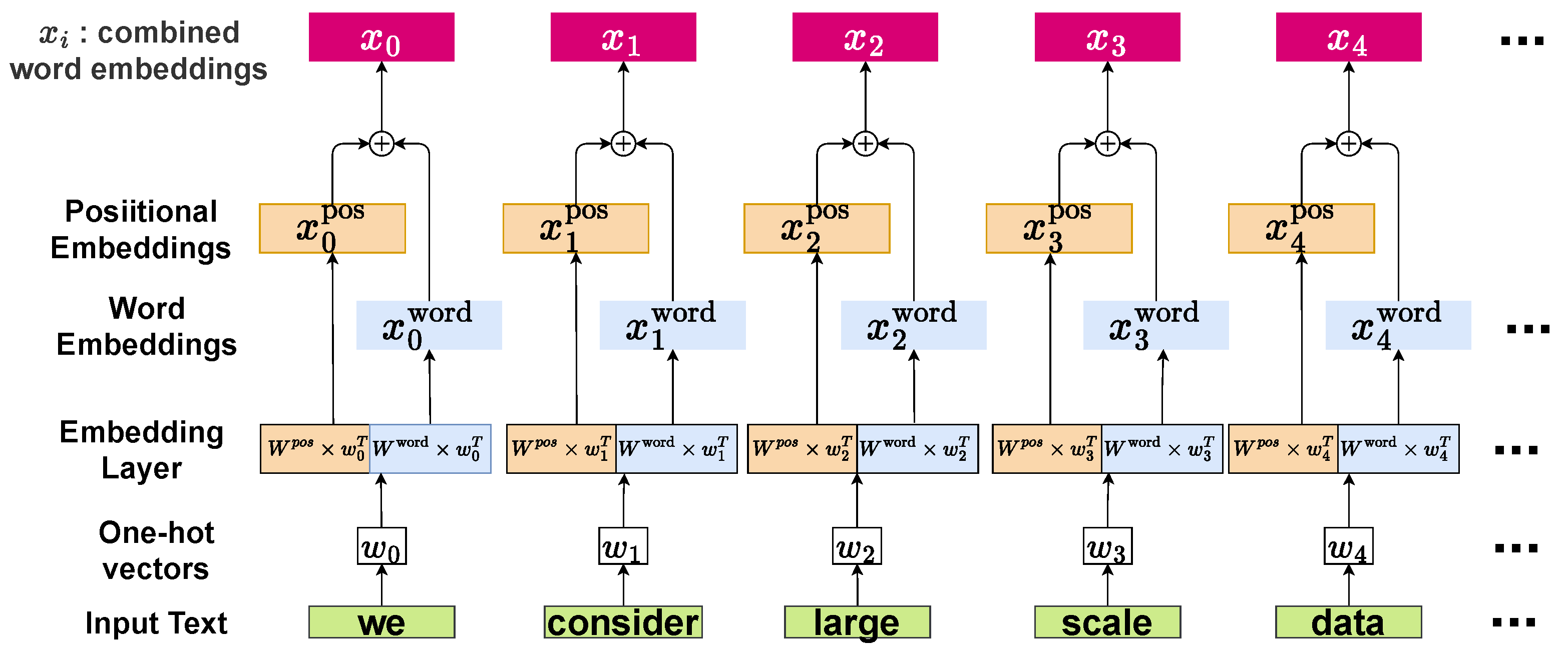
3.2.1. Embedding Block

The embedding block reduces the dimensionality of the input text and encodes the semantics and positional information of the words. This enriched and compact input representation serves to reduce computational requirements and improve performance. sBERT employs a hybrid embedding comprising a word embedding and a positional embedding. This is depicted in Figure 3.

Figure 3. Combined word and positional embeddings.

The weights in the word embedding layer are initialized using GloVe [41] and refined during training. The layer outputs the word vectors as a linear projection of the input words (Equation (1)).

$$x_i^{word}=W^{word}\times w_i$$

(1)

In Equation (1), $x_i^{word}\in \mathbb{R}$ denotes the output word vector corresponding to the ith position in the input, $w_i\in {\mathbb{R}}^{vocab\_size}$. $W^{word}\in {\mathbb{R}}^{vocab\_size\times embedding\_dim}$ denotes the word embedding matrix. Here, $embedding\_dim$ is the dimensionality of word embedding vectors. The order and position of different input words is encoded by the positional embedding layer. This layer outputs a vector by transformation using a weight matrix (Equation (2)).

$${x_i^{pos}}^T=W^{pos}\times w_i$$

(2)

Here, $x_k^{pos}\in {\mathbb{R}}^{embedding\_dim}$ is the positional embedding vector corresponding to the kth word in the input, $w_k\in {\mathbb{R}}^{vocab\_size}$. $W^{pos}\in {\mathbb{R}}^{vocab\_size\times embedding\_dim}$ denotes the weight matrix for the positional embedding layer. This matrix is initialized by weights calculated as a function of the position of a token in the input. A pair of even and odd positions in a row of the embedding matrix corresponding to the kth word, i.e., $W_{k,2i}^{pos}$ and $W_{k,2i+1}^{pos}$, is calculated using Equation (3) and Equation (4), respectively. Here, $0\le i\le embedding\_dim/2$.

$$W_{k,2i}^{pos}=sin\left({\displaystyle \frac{k}{n^{\frac{2i}{d}}}}\right)$$

(3)

$$W_{k,2i+1}^{pos}=cos\left({\displaystyle \frac{k}{n^{\frac{2i}{d}}}}\right)$$

(4)

Here, d is the intended embedding dimensionality, and n in the denominator is used to manage frequencies across the dimensions of the embeddings. By using a large value such as 10,000 for n, the frequency spectrum is spread to ensure that the embeddings can capture patterns that occur over different sequence lengths. The outputs of the two embeddings are summed to obtain an output vector. This creates a word embedding enriched with position information (Equation (5)).

$$x_i=x_i^{word}+x_i^{pos}$$

(5)

Here, $x_i\in {\mathbb{R}}^{\mathrm{embedding}\_\dim }$ represents the new hybrid embedded word vector, and $embedding\_dim$ is the dimensionality of the word embedding vector.

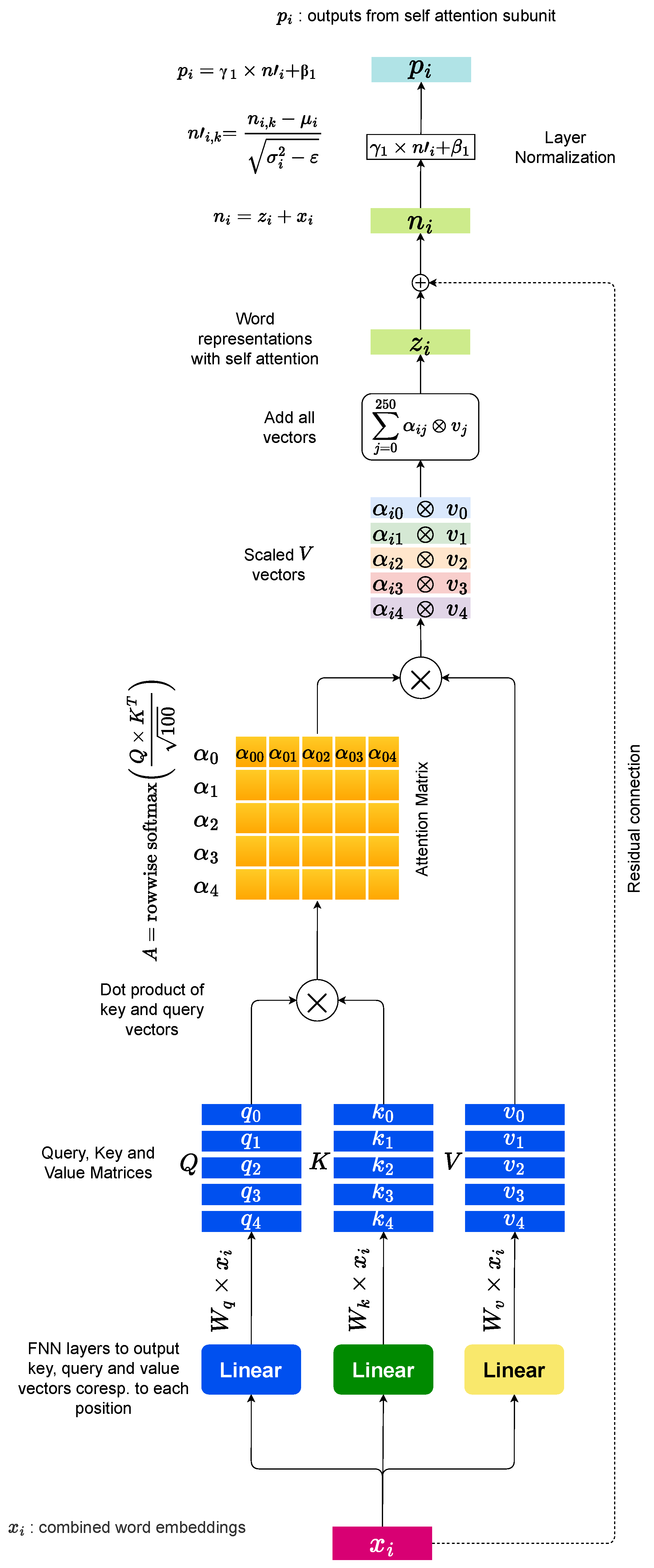
3.2.2. Query, Key, and Value Projections

To prepare the word representations for input to the encoder block (Figure 2), we use three linear transformation layers (query, key, and value) on the combined word vectors. Equations (6)–(8) depict these. The three projections are shown in Figure 3.

$$q_i={W_q\times x}_i$$

(6)

Here, $q_i\in {\mathbb{R}}^{\mathrm{embedding}\_\dim }$ denotes the query vector for the $i^{th}$ input word $x_i$, $x_i\in {\mathbb{R}}^{\mathrm{embedding}\_\dim }$ denotes the hybrid word vector obtained from the embedding block, and $W_q$ represents the weight matrix associated with generating query vectors. Also, $W_q\in {\mathbb{R}}^{\mathrm{query}\_\dim \times \mathrm{embedding}\_\dim }$ and $query\_dim$ is the dimensionality of the query vector.

$$k_i={W_k\times x}_i$$

(7)

Here, $k_i\in {\mathbb{R}}^{\mathrm{embedding}\_\dim }$ denotes the the key vector for the $i^{th}$ input word $x_i$, and $W_k$ represents the weight matrix associated with generating key vectors. Also, $W_k\in {\mathbb{R}}^{\mathrm{query}\_\dim \times \mathrm{embedding}\_\dim }$.

$$v_i={W_v\times x}_i$$

(8)

Here, $v_i\in {\mathbb{R}}^{\mathrm{embedding}\_\dim }$ denotes the the value vector for the $i^{th}$ input word $x_i$, and $W_v$ represents the weight matrix associated with generating value vectors. Also, $W_v\in {\mathbb{R}}^{\mathrm{query}\_\dim \times \mathrm{embedding}\_\dim }$.

3.2.3. Self-Attention

The purpose of the self-attention mechanism is to obtain a context-aware representation of the input words. This helps detect long-range dependencies within the input, which in turn improves model performance. The following subsections describe the self-attention mechanism employed by the proposed model to enhance word representation and hence the overall model performance.

Overview

To represent a sequence of words, self-attention connects various positions of the sequence. If the same word is surrounded, in two different instances, by different words, humans understand it differently. By self-attention, we mean attending to other words in the context when interpreting each word in a text sample.

Regularities within a natural language such as sentence structure, grammar, and semantics associated with each word (word embedding vectors) cause a model with an attention mechanism built into its architecture to learn to attend to important words within the text. Attention is learned because it is rewarding for the task that the model is trained on. Training the model on a task that requires language understanding such as text classification improves this attention mechanism. This is because training improves contextual representation (one that attends to other areas of the text). Since the contextual representation is calculated using self-attention, the representation can only be improved by improving the attention mechanism itself.

Self-Attention Mechanism

The encoder block generates an attention-based representation that can focus on specific information from a large context. The attention score for a keyword when generating a representation for a given query word is calculated by scaling the dot product $a_{ij}$ of the query vector $q_i$ and key vector $k_j$ (of dimensionality $d^k$). This is represented in Equation (9).

$$a_{ij}=q_i^{\top }{k}_j$$

(9)

$$\mathrm{score}(q_i,k_j)={\displaystyle \frac{a_{ij}}{\sqrt{d^k}}}$$

(10)

In Equation (10), $q_i$ denotes the query vector, and $k_j$ is a key vector whose attention score against $q_i$ is being determined, while $d^k$ is the dimensionality of key vectors. The three projections (query, key, and value) corresponding to each input word are calculated by using three linear transformations. To obtain the attention scores for each token (query word) in the input, its dot product with all the words (key words) in the input is calculated. The dot product is calculated between the query vector representation of the query word and the key vector representation of the keyword. Scaling of the dot product $a_{ij}$ is achieved by dividing it by the square root of the dimensionality of the key vectors $\left(d^k\right)$ to obtain a $\mathrm{score}(q_i,k_j)$ (attention score for $q_i$ against each $k_i$, as shown in Equation (10)). Scores for each query $q_i$ are subjected to a soft-max normalization to obtain the attention vector ${\alpha }_i$, as shown in Equation (11).

$${\alpha }_{ij}={\displaystyle \frac{e^{score(q_i,k_j)}}{{\sum }_j{e}^{score(q_i,k_j)}}}$$

(11)

Here, ${\alpha }_{ij}$ denotes the attention score for the ith word against the jth word. The above operations can be combined into a single matrix operation that calculates an attention matrix A, in which each row ${\alpha }_i$ represents the attention score vector for the word at the ith position in the input (Equation (12)).

$$A={\displaystyle \frac{Q\times K^T}{\sqrt{d^k}}}$$

(12)

Here, Q is the matrix, in which each row $q_i$ denotes the ith query word; similarly, K denotes the key matrix, in which each row $k_i$ denotes the ith key word. The ith row $\left(a_i\right)$ in the matrix A in Equation (12) denotes the scaled dot product of the query word $q_i$ with every key word $k_j$. Each row $a_i$ of A is subjected to soft-max to calculate ${\alpha }_i$, which makes the sum of all attention weights equal to one, i.e., ${\alpha }_i=softmax\left(a_i\right),{\sum }_j{\alpha }_{i,j}=1$. To reduce the effect of dot products growing in values, which in turn pushes the soft-max function into flat regions, the dot products are scaled by the fraction ${\displaystyle \frac{1}{\sqrt{d^k}}}$, where $d^k$ is the dimensionality of the key vector. The above steps are shown in Figure 4. Next, each value vector $v_j$ is scaled by the attention weight ${\alpha }_{i,j}$. To obtain the attention-enriched word representation for the ith position in the input ($z_i$), we scale the value vectors and sum them (Equation (13)). Figure 4 shows this diagrammatically. Here, ⊗ represents the scaling operation.

$$z_i=\sum _j({\alpha }_{i,j}\otimes v_j)$$

(13)

Figure 4. Applying the self-attention sub-unit of the encoder block to an embedded input position i (Figure 3). A single attention head has been shown for simplicity.

3.2.4. Residual Connections

Residual connections [42] in the proposed model improve model performance by addressing the problem of vanishing gradients, facilitating easier optimization, encouraging feature reuse, and leveraging the residual learning principle to focus on learning challenging parts of the mapping. Nonlinear activation functions cause the gradients to expand or disappear (depending on the weights). Skip connections theoretically provide a path that travels through the network, and gradients may also travel backward along it.

The outputs calculated by attention mechanism $\left(z_i\right)$ are added to the outputs from the encoder block $\left(x_i\right)$ to obtain $(n_i\in {\mathbb{R}}^{{\mathrm{embedding}}_{\mathrm{d}}\mathrm{im}})$, vectors that are used in the subsequent layer normalization step (Equation (14)).

$${n_i=z}_i+x_i$$

(14)

3.2.5. Layer Normalization

sBERT employs layer normalization to improve model performance by stabilizing training, reducing sensitivity to initialization, improving generalization, and facilitating faster convergence, thereby reducing the training time [43]. We first calculate ${\mu }_i$, the mean, and ${\sigma }_i^2$, the variance of each input word vector $\left(n_i\right)$, as shown in Equations (15) and (16).

$${\mu }_i={\displaystyle \frac{1}{K}}\sum _{k=1}^K{n}_{i,k}$$

(15)

Here, K represents the dimensionality of the input which, in our case, is equal to the $embedding\_dim$.

$${\sigma }_i^2={\displaystyle \frac{1}{K}}\sum _{k=1}^K{(n_{i,k}-{\mu }_i)}^2$$

(16)

Each of the K features of the word is subtracted by the mean, and the difference is divided by the square root of the standard deviation calculated above. A very small number $ϵ$ is added to the standard deviation for numerical stability. In our experiments, we use a value of 0.001 for $ϵ$. This is shown in Equation (17).

$${\widehat{n}}_{i,k}={\displaystyle \frac{n_{i,k}-{\mu }_i}{\sqrt{{\sigma }_i^2+ϵ}}}$$

(17)

As the final step in layer normalization, we scale the normalized vector $\widehat{n}$ by a factor of ${\gamma }_1$ and shift its value by ${\beta }_1$, as shown in Equation (18) and depicted in Figure 5.

$$p_i={\gamma }_1{\widehat{n}}_i+{\beta }_1$$

(18)

All of the above four steps in layer normalization can be represented as shown in Equation (19).

$$p_i={LN}_{{\gamma }_1,{\beta }_1}\left(n_i\right)$$

(19)

Figure 5. Applying an FCNN (fully connected neural network) sub-unit of the encoder block to the outputs of the self-attention sub-unit (Figure 4). The superscript of the $m^0$ output vectors denotes the attention head index (0).

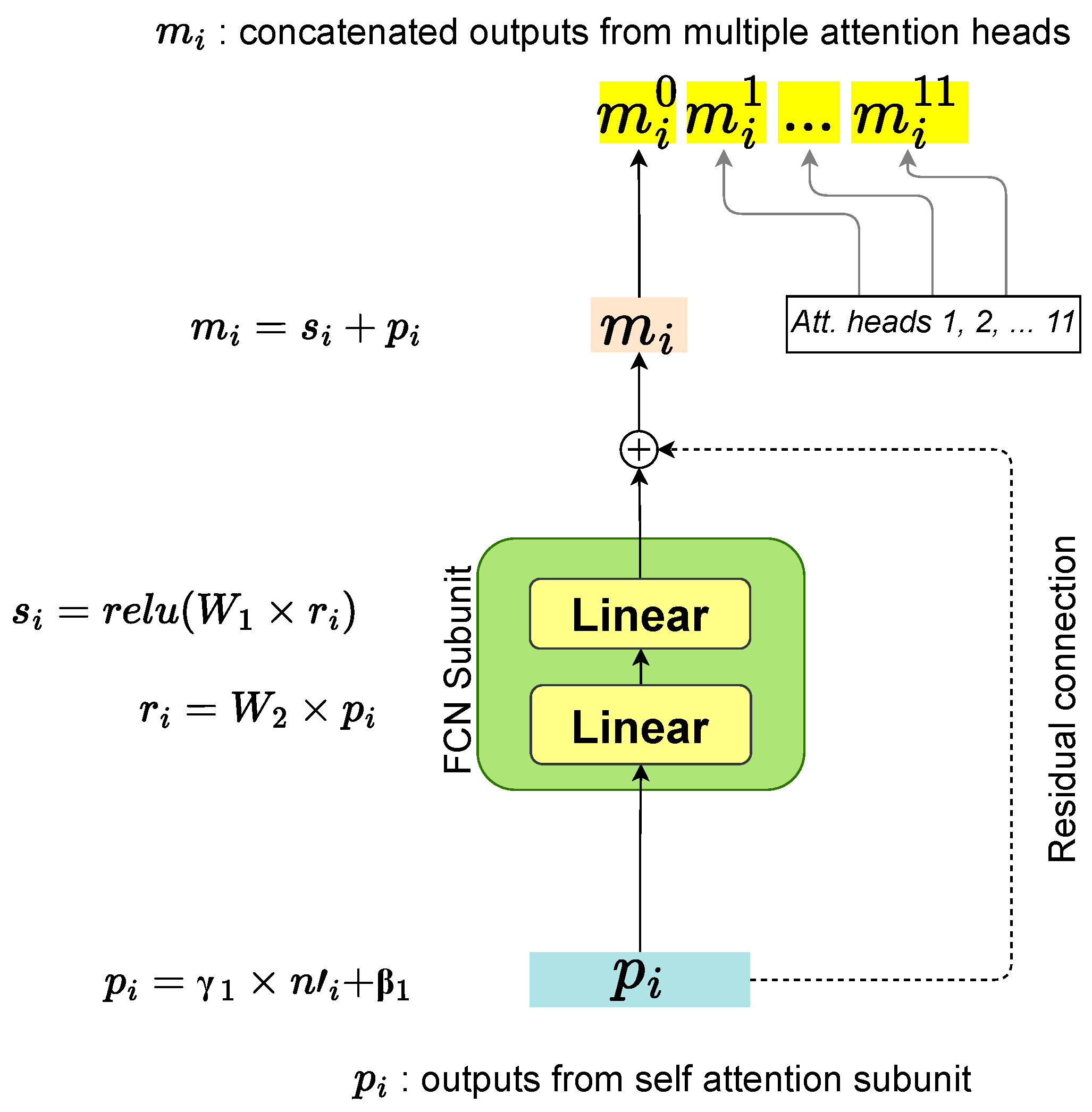
3.2.6. FCNN (Fully Connected Neural Network)

Two linear transformation layers are applied to the normalized output (Equations (20) and (21)). The fully connected layers in the model help capture and model intricate relationships within the data, leading to improved performance. Additionally, the model can extract features at different levels of granularity.

$$r_i=W_2\times p_i$$

(20)

$$s_i={relu(W}_1\times r_i)$$

(21)

Figure 5 shows the application of the FCNN to the layer normalized outputs obtained by adding scaled value projections according to the attention vector corresponding to the position.

3.2.7. Concatenating Outputs from Multiple Attention Heads

To generate a consolidated representation from multiple attention heads for each word, we concatenate the vectors obtained from all attention heads (Figure 5).

3.2.8. Residual Connections

To skip the transformations shown in Equations (20) and (21), a residual connection is employed. So, $p_i$ (the output of Equation (18) is added to $s_i$ (the output of Equation (21)). This addition gives $m_i$, the combined output (Equation (22)).

$$m_i=p_i+s_i$$

(22)

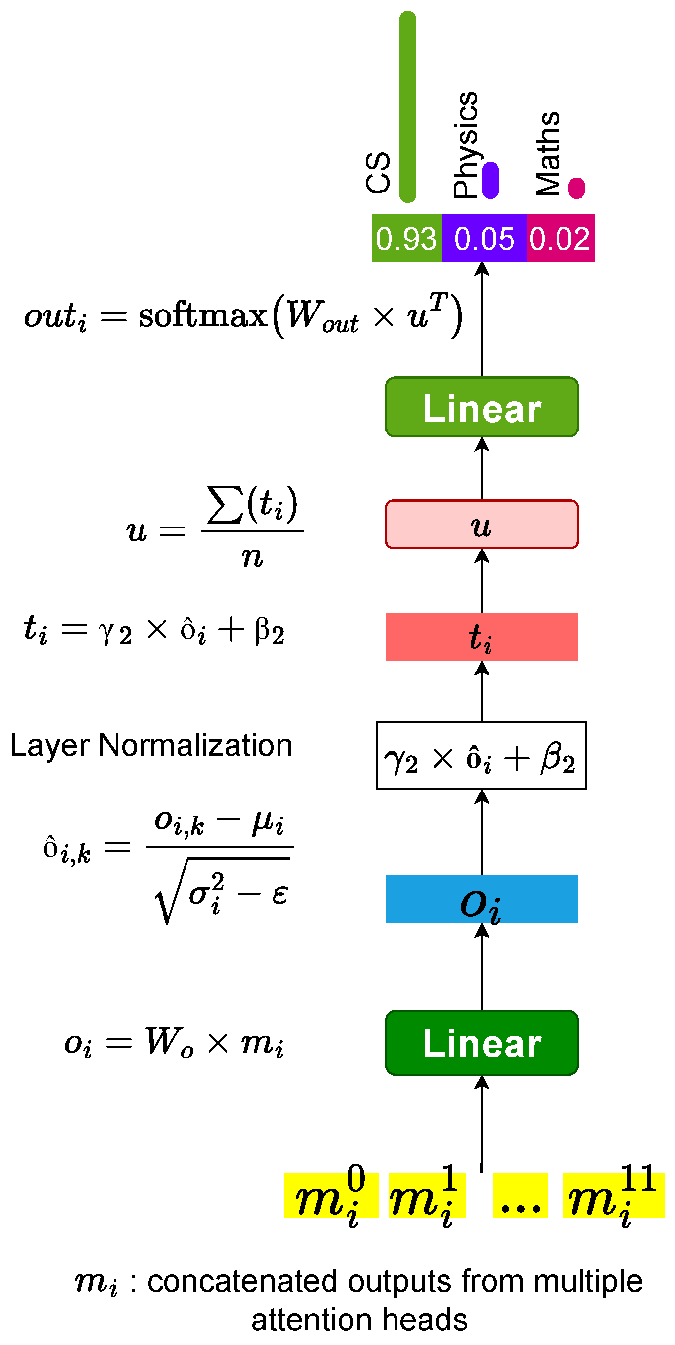
3.2.9. Combining the Representations Obtained from All Attention Heads

Outputs from multiple attention heads are consolidated by employing a linear transformation layer on the concatenated token representations obtained from all heads. This is shown in Equation (23) and illustrated in Figure 6.

$$o_i=W_0\times m_i$$

(23)

Figure 6. Obtaining a single vector representation for each position by transforming the concatenated attention outputs ($m_i$) from 12 attention heads (Figure 5) using a fully connected layer. This representation is then used for classification after normalization and averaging over positions.

The vectors $o_i$ are subjected to layer normalization and can be represented as shown in Equation (24). This is illustrated in Figure 6.

$$t_i={\mathrm{LN}}_{{\gamma }_2,{\beta }_2}\left(o_i\right)$$

(24)

3.2.10. Classification

Finally, we average all (n) positions ($t_i$) to compute the vector $\left(u\right)$ that represents the entire text, as shown in Equation (25). Averaging over all positions helps improve classification performance by capturing global context, reducing positional bias, enhancing robustness to input variations, and enhancing semantic understanding.

$$u={\displaystyle \frac{{\sum }_i^n{t}_i}{n}}$$

(25)

A soft-max-activated dense layer of neurons is used to output classification probabilities (Equations (26) and (27)).

$$y=W_{out}\times u$$

(26)

Here, $W_{out}$ represents the weight matrix of the output layer, and

$$ou{t}_i=soft-max\left(y_i\right)={\displaystyle \frac{e^{y_i}}{{\sum }_{j=1}^{nClasses}{e}^{y_j}}},$$

(27)

where $ou{t}_i\in {\mathbb{R}}^{nClasses}$. Figure 6 depicts the soft-max classification step.

4. Datasets and Experiments

The proposed model was applied to eight different datasets summarized in Table 3. For comparison, seven other deep-learning-based text classification models were also tested on the task. We ran a grid search to find the best-performing combination of hyperparameters. The grid search was run on eight datasets, and five-fold cross-validation was used to determine the best configuration for each dataset. The configuration described above showed the best performance for most datasets. The following subsections describe the datasets and the experimental setup used in the study.

Table 3. Summary of datasets used.

Dataset	Domains	Samples	Train	Test	WPS	CPS	Voc
WOS-5376	3	5736	4588	1148	209.03	1386.13	42,306
WOS-11967	7	11,967	8017	3950	201.43	1340.19	57,875
WOS-46985	7	46,985	31,479	15,506	205.27	1375.76	125,968
ArXiv	7	40,060	32,048	8012	148.21	978.67	112,452
Nature	8	49,782	24,891	24,891	175.20	1206.56	84,228
Springer	24	116,230	92,984	23,246	167.92	1128.41	22,254
Wiley	74	179,953	143,962	35,991	170.26	1150.62	113,534
COR233962	6	233,962	187,169	46,793	148.26	971.3	172,954
WIL-30628	6	30,628	24,502	6126	183.52	1230.28	43,714
SPR-50317	10	50,317	40,253	10,064	165.89	1103.97	12,531

Notes: Domains: Number of classes, Samples: Number of samples, Train: Number of training samples, Test: Number of testing samples, WPS: Words per sample (mean), CPS: Characters per sample (mean), Voc: Size of the vocabulary.

4.1. Datasets

Ten different datasets comprising abstracts of research papers were used in the study. In addition to the three Web of Science (WOS) datasets [7], we created seven new SLC datasets for the experiments. The following subsections describe the datasets.

4.1.1. WOS

The WOS datasets [7] consist of $46,958$ paper abstracts from 134 categories and 7 subcategories.

4.1.2. ArXiv

The dataset was gathered from ArXiv [44], an online preprint repository. It includes works in mathematical finance, electrical engineering, math, quantitative biology, physics, statistics, economics, astronomy, and computer science. There are 7 categories and 146 subcategories.

4.1.3. Nature

The dataset contains 49,782 abstracts from [45], and it is divided into 8 categories and 102 subcategories.

4.1.4. Springer

This dataset contains 116,230 abstracts from Springer [46], which are divided into 24 categories and 117 subcategories. A subset (SPR-50317) consisting of the largest 6 categories was also created.

4.1.5. Wiley

The dataset contains 179,953 samples and was obtained from Wiley [47]. It contains 494 categories and 74 subcategories. A subset (WIL-30628) consisting of the largest 6 categories was also created.

4.1.6. COR233962

COR233962 has 233,962 abstracts divided into 6 categories. It was obtained from the repository made available by Cornell University [48].

The datasets differ in domains, sample sizes for training and testing, average words and characters per sample, and vocabulary size. These factors can affect the performance of text classification models. Generally, larger and more diverse datasets enhance model performance. Table 3 outlines the datasets used in this study.

4.2. Experimental Setup

Experiments for the study were performed on a hardware configuration that uses an Intel® Xeon® CPU @ 2.30 GHz, 12 GB of RAM, and approximately 358 GB of free disk space (Table 4). It also uses an NVIDIA Tesla T4 GPU. Table 5 lists the training times of different models. Code for the proposed model can be found online (Code: https://github.com/munziratcoding/sBERT, accessed on 11 July 2024). The following subsections present a detailed account of the experimental setup.

Table 4. System configuration.

Property	Value
Operating System	Linux-6.1.85+-x86_64-with-glibc2.35
Python Version	3.10.12
CPU Count	2
CPU Model	Intel® Xeon® CPU @ 2.30 GHz
GPU Count	1
GPU Model	1 x Tesla T4
Longitude	−79.9746
Latitude	32.8608
RAM	12.7 GB

Table 5. Training times for sBERT on different datasets.

$\mathbf{Dataset}$	WOS-5736	WOS-11967	WOS-46985	$\mathbf{Nature}$	$\mathbf{Springer}$	$\mathbf{ArXiv}$	$\mathbf{Wiley}$	COR-233962	WIL-30628	SPR-50317
Time (s)	157.2688	286.5306	713.4463	361.6975	721.5509	500.1951	4233.135	2299.827	460.3575	287.246

4.2.1. Data Acquisition

To acquire some of the datasets, an HTTP request was sent to retrieve the required data, and the HTML content was retrieved using the HTTP library. The lxml library was then used to parse the HTML content and extract the abstracts and categories. The BeautifulSoup library was used to transform the data into a Pandas dataframe that was stored as a CSV file for further processing and analysis.

The datasets were sourced from individual repositories, ensuring consistency in class distribution between samples and their respective sources. In instances where certain classes contained an insufficient number of samples, exacerbating class imbalance, such classes were omitted from the datasets. Additionally, the variation in the number of classes within the created datasets aimed to enhance diversity.

4.2.2. Data Cleaning and Preprocessing

Special characters were filtered out from the abstracts, and tokenization (vocabulary size of 20,000) was performed. The input was restricted to the length of 250 tokens. This was achieved by padding and truncation.

4.2.3. Data Splitting for Training, Validation, and Testing

The datasets were randomly shuffled to remove ordering bias and then split into training and testing subsets using an 80:20 ratio. The training subsets were used for model training, while the test subsets were used for performance evaluation.

4.2.4. Hyperparameter Selection

For hyperparameter selection for sBERT, we ran a grid search over the ranges of hyperparameters, such as the number of attention heads [1–12], number of encoder blocks [1–12], embedding size [100–300], and the size of the fully connected and neural network layers [32–512]. The configuration discussed in the proposed model showed optimal performance across most datasets.

4.2.5. Training Details

The Adam optimizer with a learning rate of $0.01$ was employed to train sBERT. A batch size of 16 and 100 epochs with early stopping was used. Figure 7 and Figure 8 show the training graphs obtained during training sBERT on the WOS-46985 and COR-233962 datasets. Training times on different datasets for sBERT are listed in Table 5.

Figure 7. Training graphs for sBERT on the WIL-30628 dataset.

Figure 8. Training graphs for sBERT on the WOS-46985 dataset.

4.2.6. Performance Metric

Classification accuracy percentage, a measure of the percentage of correctly classified instances in a dataset, was employed. It is defined as the ratio of the number of correctly classified instances to the total number of instances in the dataset, multiplied by 100. Classification accuracy can be described mathematically as shown in Equation (28):

$$\mathrm{Classification}\mathrm{Accuracy}={\displaystyle \frac{\mathrm{No}.\mathrm{of}\mathrm{correct}\mathrm{predictions}}{\mathrm{Total}\mathrm{No}.\mathrm{of}\mathrm{predictions}}}\times 100\%.$$

(28)

5. Results and Discussion

We evaluate the performance of sBERT against several other deep-learning text classification techniques using classification accuracy percentages. Section 5.1 contrasts the parameter space sizes of different transformer-based models with the proposed model. In Section 5.2, we compare different models based on their carbon emissions. Section 5.3 explores the classification accuracy outcomes for various datasets. Finally, in Section 5.4, we present the results of hypothesis testing.

5.1. Parameter Space Comparison

Table 2 shows a comparison of various language models based on their parameter space size, which is an important consideration when selecting a model for a specific task.

As described in Table 2, BERT base, XLNet, and RoBERTa base all have 12 transformer layers, with varying hidden sizes, attention heads, and number of parameters. Models such as BERT large have 24 encoder layers, with larger hidden sizes and attention heads than their base counterparts, resulting in significantly larger parameter spaces. BERT large has 340 million parameters, while RoBERTa large has 355 million parameters. DistilBERT and ALBERT are both designed to be smaller and more efficient versions of BERT. DistilBERT has only six transformer layers, resulting in a smaller parameter space of 66 million parameters. ALBERT has 24 transformer layers like BERT large, but with a smaller hidden size and fewer attention heads, resulting in a much smaller parameter space of only 18 million parameters.

sBERT uses a single lightweight encoder block, a hidden size of 100, and 12 attention heads. This ensures a very small parameter space of $11.9$ million. sBERT’s parameter efficiency makes it optimal for applications involving text classification tasks. This also makes sBERT more suitable for low-resource applications and reduces the carbon footprint associated with training and fine-tuning more complex models (Table 6).

Table 6. Energy consumption and carbon emission of various models.

Model	Duration	Energy Consumption (kWh)	Carbon Emission (kg CO2)
ALBERT [15]	844.3437219	0.018017887	0.008806693
BERT [11]	828.3376598	0.019312801	0.009439614
ELECTRA [34]	5381.362884	0.15103994	0.043122468
DistilBERT [16]	8414.990516	0.247839145	0.034387638
RoBERTa [14]	1647.26625	0.038005353	0.005273236
sBERT	84.86049414	0.001797255	0.000878453

5.2. Carbon Emissions Comparison

The carbon emissions for training a deep learning model largely depend on the model’s complexity and size, including the number of parameters and layers, which directly influence computational demands. Larger, more intricate models require more processing power and memory, leading to higher energy consumption. Additionally, the duration of training, dictated by the number of epochs and iterations, significantly impacts overall energy use. Efficient software implementation and optimization algorithms can mitigate some of these demands, but ultimately, more complex and sizable models inherently consume more energy, contributing to greater carbon emissions. Table 6 compares different models in terms of their carbon emissions. Measurements have been taken for training the models for 20 epochs in a training environment with the specifications in Table 4.

Carbon Emissions Calculation

• Power Consumption (Watts)
  Power consumption is the total power used by the hardware resources (CPU, GPU, and RAM) during model training. It can be calculated using Equation (29):

  $$P_{\mathrm{total}}=P_{\mathrm{CPU}}+P_{\mathrm{GPU}}+P_{\mathrm{RAM}},$$

  (29)

  where $P_{\mathrm{CPU}}$, $P_{\mathrm{GPU}}$, and $P_{\mathrm{RAM}}$ represent the power consumption of the CPU, GPU, and RAM, respectively.
• Energy Consumption (kWh)
  Energy consumption is the total amount of power consumed over a period of time. It is given by Equation (30),

  $$E_{\mathrm{total}}=P_{\mathrm{total}}\times t,$$

  (30)

  where t is the duration of the model training in hours.
• Carbon Emission (kg CO₂ per kWh)
  The carbon emission is calculated by multiplying the energy consumption by the carbon intensity of the electricity grid. The carbon emission can be calculated using Equation (31),

  $$\mathrm{Carbon}\mathrm{Emission}=E_{\mathrm{total}}\times CI,$$

  (31)

  where $CI$ is the carbon intensity factor.

5.3. Performance Comparison

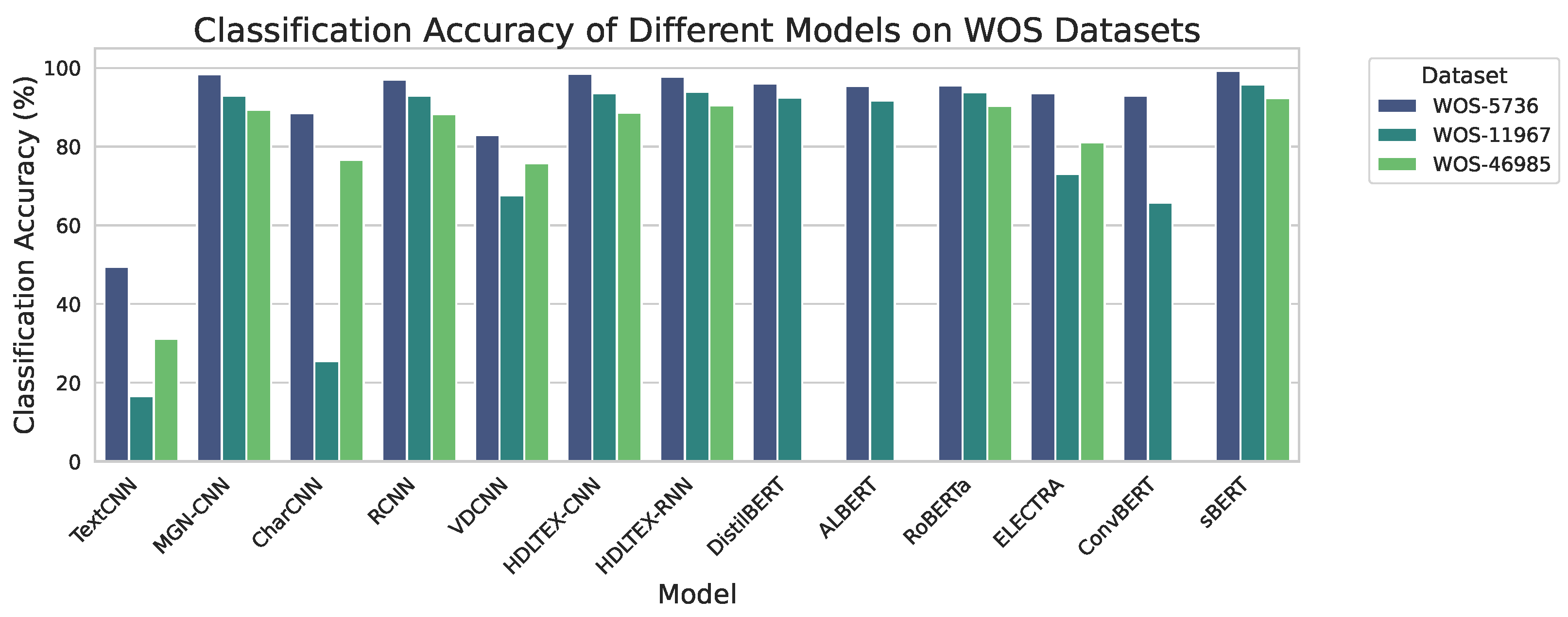
In this section, we report evaluation results for various models on the WOS datasets and the other seven datasets.

5.3.1. WOS Datasets

Table 7 lists the classification accuracy percentage measurements of different models across the three WOS datasets. Figure 9 presents the results graphically. Figure 10 shows the confusion matrix of the proposed model on the largest of the WOS datasets, WOS-46985. Table 8 and Table 9 list the Precision, Recall, and F1 scores corresponding to the seven classes corresponding to the two confusion matrices.

Table 7. Results (classification accuracy %) on the WOS datasets.

Model	WOS-5736	WOS-11967	WOS-46985
TextCNN [4]	49.46	16.55	31.13
MGN-CNN [17]	98.41	92.94	89.33
CharCNN [19]	88.48	25.45	76.59
RCNN [37]	97.07	92.94	88.2
VDCNN [20]	82.9	67.64	75.76
HDLTEX-CNN [7]	98.47	93.52	88.67
HDLTEX-RNN [7]	97.82	93.98	90.45
DistilBERT [16]	96.08	92.4	-
ALBERT [15]	95.38	91.65	-
RoBERTa [14]	95.56	93.82	90.32
ELECTRA [34]	93.55	73.1	81.05
ConvBERT [33]	92.94	65.75	-
sBERT	99.21	95.85	92.36

Figure 9. Graph showing classification accuracy (percentage) of different models on the WOS datasets.

Figure 10. Confusion matrices for sBERT on the dataset WOS-46985 and RCNN on WOS-46985 for comparison. For analysis, see Table 8 and Table 9.

Table 8. Precision, Recall, and F1 scores for RCNN on WOS-46985 (Figure 10).

	CS	ECE	Psych	MAE	Civil	Med	Biochem
Precision	0.903837	0.916994	0.87562	0.776646	0.86635	0.890251	0.890887
Recall	0.995567	0.993842	0.996837	0.997282	0.995622	0.998372	0.995129
F1 score	0.947487	0.953873	0.932305	0.873243	0.926498	0.941217	0.940127

Notes: CS: Computer science, ECE: Electronics and communication engineering, Psych: Psychology, MAE: Mechanical and Aerospace Engineering, Civil: Civil Engineering, Med: Medicine, Biochem: Biochemistry.

Table 9. Precision, Recall, and F1 scores for sBERT on WOS-46985 (Figure 10).

	CS	ECE	Psych	MAE	Civil	Med	Biochem
Precision	0.919893	0.932343	0.89906	0.9287	0.96131	0.961392	0.923961
Recall	0.994915	0.992477	0.996373	0.988381	0.981849	0.994745	0.993397
F1 score	0.955935	0.961471	0.945219	0.957612	0.971471	0.977784	0.957421

Notes: CS: Computer science, ECE: Electronics and communication engineering, Psych: Psychology, MAE: Mechanical and Aerospace Engineering, Civil: Civil Engineering, Med: Medicine, Biochem: Biochemistry.

5.3.2. Discussion

The experimental results offer insights into the performance of various text classification models across the three datasets: WOS-5736, WOS-11967, and WOS-46985. Each model’s classification accuracy percentages were evaluated on these datasets. Among the models assessed, TextCNN exhibited relatively modest performance, achieving the highest accuracy on WOS-5736 at 49.46%. However, its overall performance across datasets was less than satisfactory, implying limitations in capturing intricate relationships within the data. Conversely, the Multi-Group Norm Constraint CNN (MGN-CNN) demonstrated better performance across the datasets, most notably on WOS-5736, with an accuracy of 98.41%.

The Character-level CNN (CharCNN) displayed moderate performance, with the highest accuracy on WOS-5736 at 88.48%. Its performance may be attributed to its ability to exploit character-level information, making it suitable for datasets where such details are pivotal. In contrast, the Recurrent CNN (RCNN) showcased robust performance across the three datasets, suggesting its competence in capturing both local and sequential patterns in the data.

The Very Deep CNN (VDCNN) showed the highest accuracy on WOS-5736 at 82.9%. However, deep models like VDCNN often entail higher computational requirements. The hybrid models, HDLTEX-CNN and HDLTEX-RNN, demonstrated strong performance, particularly on WOS-5736 and WOS-11967.

Most notably, the proposed model, sBERT, consistently outperformed other models across the datasets, achieving the highest accuracy on WOS-5736 at 99.21%. This superior performance is achieved by the incorporation of a multi-headed attention mechanism that enables sBERT to focus on the most salient portions of the text. Moreover, the utilization of word embeddings enriched by position information contributes to its success by effectively capturing semantic relationships and context—a vital aspect of text classification tasks.

5.3.3. Other Datasets

Table 10 lists the classification accuracy percentage measurements across the Nature, Springer, ArXiv, Wiley, and CornellArXiv datasets. Figure 10 shows confusion matrices for sBERT and RCNN on the WOS-46985 dataset. Figure 11 presents the results graphically.

Table 10. Classification accuracy (%) comparison on other datasets.

Model	Nature	Springer	ArXiv	Wiley	COR233962	SPR-50317	WIL-30628
TextCNN [4]	33.79	27.7	26.26	8.15	88.74%	90.06%	75.69
MGN-CNN [17]	57.23	100	85.35	52.04	95.93	98.5	93.2
CharCNN [19]	51.23	61.6	80.53	7.82	53.22	94.09	91.62
RCNN [37]	52.21	85	83.32	62.1	93.81	99.0	94.63
VDCNN [20]	53.44	63	66.11	49.5	54.91	30.3	20.66
HDLTEX-CNN [7]	60.12	99.98	85.84	50.81	91.6	100	94.79
HDLTEX-RNN [7]	61.83	100	84.26	43.39	92.15	80.85	85.11
sBERT	63.2	100	85.94	70.54	93.17	100	94.6

Figure 11. Graph showing classification accuracy (percentage) of different models on the other datasets.

5.3.4. Discussion

The experimental results present a comprehensive evaluation of various text classification models applied across the five distinct datasets: Nature, Springer, ArXiv, Wiley, and CornellArXiv.

TextCNN, the first model considered, demonstrates variable performance across datasets, achieving relatively lower accuracy percentages. It notably struggles on the Wiley dataset, attaining an accuracy of 8.15%. However, it exhibits more robust performance on the COR233962 dataset, reaching an accuracy of 85.06%. These variations in performance suggest that TextCNN may face challenges in datasets with diverse characteristics.

Conversely, the Multi-Group Norm Constraint CNN (MGN-CNN) showcases consistent and robust performance across all datasets, with notable accuracy percentages of 100% on Springer and 85.35% on ArXiv.

The Character-level CNN (CharCNN) exhibits moderate performance, with its highest accuracy observed on the ArXiv dataset at 80.53%. However, it faces challenges in the Wiley dataset, where it attains an accuracy of 7.82%. These results may be attributed to CharCNN’s reliance on character-level information, which may be less relevant or informative in certain datasets.

The Recurrent CNN (RCNN) achieves competitive accuracy percentages across datasets, notably reaching 85% on Springer and 83.32% on ArXiv. Its recurrent architecture enables it to effectively capture sequential patterns in the data, which contributes to its adaptability.

The Very Deep CNN (VDCNN) demonstrates its highest accuracy on Springer at 63%. Nevertheless, it encounters challenges in the ArXiv dataset, where it achieves an accuracy of 66.11%. These variations in performance suggest that the depth of the model may not universally benefit all datasets.

The models HDLTEX-CNN and HDLTEX-RNN perform well across most datasets, with notable accuracy percentages. These models effectively leverage CNN and RNN architectures, showcasing their adaptability and utility in various text classification scenarios.

The proposed model, sBERT, performs well in all datasets, achieving the highest accuracy on Springer at 100% and on ArXiv at 85.94%. sBERT’s exceptional performance underscores its versatility, which can be attributed to its multi-headed attention-based architecture and utilization of hybrid word and positional embeddings. These qualities enable sBERT to excel in various domains and dataset characteristics. The exceptional performance of sBERT across different datasets underscores its robustness and generalizability, suggesting its effectiveness in handling diverse domains and dataset sizes. sBERT’s parameter efficiency is particularly crucial in mitigating the computational resources and carbon footprint associated with large-scale language models. The proposed model requires just 15.7 MB of memory and takes 0.06 s (average over inference times for 100 samples) to predict in the training environment (described in Section 4.2).

5.4. Hypothesis Testing

Hypothesis testing was performed to compare sBERT with other models using the $2\times 5$ cross-validation method. For example, comparison with the RCNN model on the WOS-5736 dataset yielded the following results.

5.4.1. Accuracy Measurements of Compared Models

The accuracy measurements of the two models for the 10 splits in $2\times 5$ cross-validation are presented in Table 11.

Table 11. Accuracy measurements of RCNN and sBERT for the 10 splits in $2\times 5$ cross-validation.

Model	Split 1	Split 2	Split 3	Split 4	Split 5	Split 6	Split 7	Split 8	Split 9	Split 10
RCNN	0.8434	0.6172	0.8978	0.7528	0.6688	0.7298	0.8016	0.7402	0.6492	0.7720
sBERT	0.9477	0.9390	0.9571	0.9386	0.9460	0.9467	0.9383	0.9529	0.9456	0.9550

5.4.2. Paired t-Test

• t-statistic: $-7.48$
• p-value: $3.78\times {10}^{-5}$

The paired t-test statistic is obtained using Equation (32):

$$t={\displaystyle \frac{\overline{d}}{s_d/\sqrt{n}}},$$

(32)

where:

$\overline{d}$ denotes the average difference between paired observations;

$s_d$ denotes the standard deviation of the differences;

n is the number of pairs.

5.4.3. Interpretation of the Results

The paired t-test is used to decide if there is a statistically significant difference between the means of two related groups (in this case, the classification accuracy of sBERT and RCNN across the different splits).

• t-statistic: The t-statistic of $-7.48$ is a measure of the difference between the two groups relative to the variability observed within the groups. The large negative value shows that the accuracy of sBERT is significantly different from that of RCNN.
• p-value: The p-value of $3.78\times {10}^{-5}$ is much lower than the significance level threshold (0.05), suggesting that the difference in classification accuracy between sBERT and RCNN is statistically significant. This indicates that there is strong evidence to reject the null hypothesis (there is no difference in performance between the two models).

The low p-value in the test provides strong evidence against the null hypothesis, indicating that the observed difference in classification accuracy is highly unlikely to be due to random chance.

6. Conclusions and Future Work

In this study, we proposed sBERT, a parameter-efficient transformer model tailored for the classification of scientific literature. Through extensive experiments on multiple datasets, sBERT has been shown to outperform traditional models in both accuracy and efficiency. Our findings highlight the advantages of the multi-headed attention mechanism and optimized embeddings used in sBERT. Furthermore, the reductions in memory use, training and inference times, and carbon footprint emphasize the model’s efficiency and environmental benefits. Future work will explore the application of sBERT to other text classification domains and further optimize its architecture for even greater performance.

References

- Ware, M.; Mabe, M. The STM Report: An Overview of Scientific and Scholarly Journal Publishing; Technical Report 4; International Association of Scientific, Technical and Medical Publishers: Oxford, UK, 2015. [Google Scholar]
- Jinha, A.E. Article 50 Million: An Estimate of the Number of Scholarly Articles in Existence. Learn. Publ. 2010, 23, 258–263. [Google Scholar] [CrossRef]
- National Center for Education Statistics. Doctor’s Degrees Conferred by Postsecondary Institutions, by Field of Study: Selected Years, 1970-71 through 2018-19. Digest of Education Statistics, 2019. Available online: https://nces.ed.gov/programs/digest/d21/tables/dt21_324.10.asp (accessed on 15 June 2024).
- Kim, Y. Convolutional Neural Networks for Sentence Classification. In Proceedings of the EMNLP, Doha, Qatar, 25–29 October 2014. [Google Scholar]
- Georgakopoulos, S.V.; Tasoulis, S.K.; Vrahatis, A.G.; Plagianakos, V.P. Convolutional Neural Networks for Toxic Comment Classification. In Proceedings of the 10th Hellenic Conference on Artificial Intelligence, Patras, Greece, 9–12 July 2018; pp. 1–6. [Google Scholar]
- Hughes, M.; Li, I.; Kotoulas, S.; Suzumura, T. Medical Text Classification Using Convolutional Neural Networks. Stud. Health Technol. Inform. 2017, 235, 246–250. [Google Scholar]
- Kowsari, K.; Brown, D.E.; Heidarysafa, M.; Meimandi, K.J.; Gerber, M.S.; Barnes, L.E. HDLTex: Hierarchical Deep Learning for Text Classification. In Proceedings of the 16th IEEE International Conference on Machine Learning and Applications (ICMLA), Cancun, Mexico, 18–21 December 2018; Volume 2018, pp. 364–371. [Google Scholar]
- Aripin; Agastya, W.; Huda, S. Multichannel Convolutional Neural Network Model to Improve Compound Emotional Text Classification Performance. IAENG Int. J. Comput. Sci. 2023, 50, 866. [Google Scholar]
- Zhou, P.; Qi, Z.; Zheng, S.; Xu, J.; Bao, H.; Xu, B. Text classification improved by integrating bidirectional LSTM with two-dimensional max pooling. In Proceedings of the COLING 2016, the 26th International Conference on Computational Linguistics: Technical Papers, Osaka, Japan, 11–16 December 2016; pp. 3485–3495. [Google Scholar]
- McCann, B.; Bradbury, J.; Xiong, C.; Socher, R. Learned in Translation: Contextualized Word Vectors. In Proceedings of the Advances in Neural Information Processing Systems, Long Beach, CA, USA, 4–9 December 2017. [Google Scholar]
- Devlin, J.; Chang, M.; Lee, K.; Toutanova, K. BERT: Pre-training of Deep Bidirectional Transformers for Language Understanding. In Proceedings of the 2019 Conference of the North American Chapter of the Association for Computational Linguistics: Human Language Technologies, Volume 1 (Long and Short Papers), Minneapolis, MN, USA, 2–7 June 2019; pp. 4171–4186. [Google Scholar] [CrossRef]
- Vaswani, A.; Shazeer, N.; Parmar, N.; Uszkoreit, J.; Jones, L.; Gomez, A.N.; Kaiser, L.; Polosukhin, I. Attention is all you need. In Proceedings of the Advances in Neural Information Processing Systems, Long Beach, CA, USA, 4–9 December 2017; pp. 5998–6008. [Google Scholar]
- Yang, Z.; Dai, Z.; Yang, Y.; Carbonell, J.; Salakhutdinov, R.R.; Le, Q.V. XLNet: Generalized Autoregressive Pretraining for Language Understanding. In Proceedings of the Advances in Neural Information Processing Systems, Vancouver, BC, Canada, 8–14 December 2019; Wallach, H., Larochelle, H., Beygelzimer, A., d’Alché-Buc, F., Fox, E., Garnett, R., Eds.; Curran Associates, Inc.: Sydney, Australia, 2019; Volume 32. [Google Scholar]
- Liu, Y.; Ott, M.; Goyal, N.; Du, J.; Joshi, M.; Chen, D.; Levy, O.; Lewis, M.; Zettlemoyer, L.; Stoyanov, V. RoBERTa: A Robustly Optimized BERT Pretraining Approach. arXiv 2019. [Google Scholar] [CrossRef]
- Lan, Z.; Chen, M.; Goodman, S.; Gimpel, K.; Sharma, P.; Soricut, R. ALBERT: A lite BERT for self-supervised learning of language representations. In Proceedings of the 8th International Conference on Learning Representations, Addis Ababa, Ethiopia, 26–30 April 2020. [Google Scholar]
- Sanh, V.; Debut, L.; Chaumond, J.; Wolf, T. DistilBERT, a distilled version of BERT: Smaller, faster, cheaper and lighter. arXiv 2019. [Google Scholar] [CrossRef]
- Zhang, Y.; Roller, S.; Wallace, B.C. MGNC-CNN: A Simple Approach to Exploiting Multiple Word Embeddings for Sentence Classification. arXiv 2016, arXiv:1603.00968. [Google Scholar]
- Wu, H.L.X.; Cai, Y.; Xu, J.; Li, Q. Combining Machine Learning and Lexical Features for Readability Assessment of User Generated Content. In Proceedings of the COLING, Dublin, Ireland, 23–29 August 2014. [Google Scholar]
- Zhang, X.; Zhao, J.; LeCun, Y. Character-level Convolutional Networks for Text Classification. In Proceedings of the Advances in Neural Information Processing Systems, Montreal, QC, Canada, 7–12 December 2015; Volume 28, pp. 649–657. [Google Scholar]
- Conneau, A.; Schwenk, H.; Cun, Y.L.; Barrault, L. Very deep convolutional networks for text classification. In Proceedings of the 15th Conference of the European Chapter of the Association for Computational Linguistics, EACL 2017—Proceedings of Conference, Valencia, Spain, 3–7 April 2017; Volume 1, pp. 1107–1116. [Google Scholar] [CrossRef]
- Johnson, R.; Zhang, T. Convolutional Neural Networks for Text Categorization: Shallow Word-level vs. Deep Character-level. arXiv 2016, arXiv:1609.00718. [Google Scholar]
- Wang, H.; He, J.; Zhang, X.; Liu, S. A short text classification method based on N-gram and CNN. Chin. J. Electron. 2020, 29, 248–254. [Google Scholar] [CrossRef]
- Soni, S.; Chouhan, S.S.; Rathore, S.S. TextConvoNet: A convolutional neural network based architecture for text classification. Appl. Intell. 2023, 53, 14249–14268. [Google Scholar] [CrossRef] [PubMed]
- Mandelbaum, A.; Shalev, A. Word Embeddings and Their Use In Sentence Classification Tasks. arXiv 2016, arXiv:1610.08229. [Google Scholar]
- Senarath, Y.; Thayasivam, U. DataSEARCH at IEST 2018: Multiple Word Embedding based Models for Implicit Emotion Classification of Tweets with Deep Learning. In Proceedings of the 9th Workshop on Computational Approaches to Subjectivity, Sentiment and Social Media Analysis, Brussels, Belgium, October 2018; Balahur, A., Mohammad, S.M., Hoste, V., Klinger, R., Eds.; Association for Computational Linguistics: Stroudsburg, PA, USA, 2018; pp. 211–216. Available online: https://aclanthology.org/W18-6230 (accessed on 11 July 2024).
- Yang, Z.; Yang, D.; Dyer, C.; He, X.; Smola, A.; Hovy, E. Hierarchical Attention Networks for Document Classification. In Proceedings of the 2016 Conference of the North American Chapter of the Association for Computational Linguistics: Human Language Technologies, San Diego, CA, USA, 12–17 June 2016; pp. 1480–1489. [Google Scholar] [CrossRef]
- Zhou, X.; Wan, X.; Xiao, J. Attention-based LSTM network for cross-lingual sentiment classification. In Proceedings of the 2016 Conference on Empirical Methods in Natural Language Processing, Austin, TX, USA, 1–5 November 2016; pp. 247–256. [Google Scholar] [CrossRef]
- Bahdanau, D.; Cho, K.; Bengio, Y. Neural Machine Translation by Jointly Learning to Align and Translate. In Proceedings of the 3rd International Conference on Learning Representations, ICLR 2015, San Diego, CA, USA, 7–9 May 2015. [Google Scholar]
- Hassan, A.; Mahmood, A. Convolutional recurrent deep learning model for sentence classification. IEEE Access 2018, 6, 13949–13957. [Google Scholar] [CrossRef]
- Gonçalves, S.; Cortez, P.; Moro, S. A Deep Learning Approach for Sentence Classification of Scientific Abstracts. In Discovery Science; Lecture Notes in Computer Science; Springer: Cham, Switzerland, 2018; Volume 11198, pp. 21–35. [Google Scholar] [CrossRef]
- Jin, D.; Szolovits, P. Hierarchical Neural Networks for Sequential Sentence Classification in Medical Scientific Abstracts. In Proceedings of the 2018 Conference on Empirical Methods in Natural Language Processing, Brussels, Belgium, 31 October–4 November 2018; pp. 2561–2572. [Google Scholar] [CrossRef]
- Yang, Z.; Emmert-Streib, F. Threshold-learned CNN for multi-label text classification of electronic health records. IEEE Access 2023, 11, 17574–17583. [Google Scholar] [CrossRef]
- Jiang, Z.H.; Yu, W.; Zhou, D.; Chen, Y.; Feng, J.; Yan, S. Convbert: Improving bert with span-based dynamic convolution. Adv. Neural Inf. Process. Syst. 2020, 33, 12837–12848. [Google Scholar]
- Clark, K.; Luong, M.T.; Le, Q.V.; Manning, C.D. ELECTRA: Pre-training Text Encoders as Discriminators Rather Than Generators. In Proceedings of the International Conference on Learning Representations, Addis Ababa, Ethiopia, 26–30 April 2020. [Google Scholar]
- He, P.; Liu, X.; Gao, J.; Chen, W. Deberta: Decoding-enhanced bert with disentangled attention. In Proceedings of the International Conference on Learning Representations, Addis Ababa, Ethiopia, 26–30 April 2020. [Google Scholar]
- He, P.; Gao, J.; Chen, W. DeBERTaV3: Improving DeBERTa using ELECTRA-Style Pre-Training with Gradient-Disentangled Embedding Sharing. In Proceedings of the Eleventh International Conference on Learning Representations, Kigali, Rwanda, 1–5 May 2023. [Google Scholar]
- Lai, S.; Xu, L.; Liu, K.; Zhao, J. Recurrent convolutional neural networks for text classification. In Proceedings of the National Conference on Artificial Intelligence, Austin, TX, USA, 25–30 January 2015; Volume 3, pp. 2267–2273. [Google Scholar]
- Sun, Z.; Yu, H.; Song, X.; Liu, R.; Yang, Y.; Zhou, D. MobileBERT: A Compact Task-Agnostic BERT for Resource-Limited Devices. In Proceedings of the 58th Annual Meeting of the Association for Computational Linguistics, Online, 5–10 July 2020; Jurafsky, D., Chai, J., Schluter, N., Tetreault, J., Eds.; pp. 2158–2170. [Google Scholar] [CrossRef]
- Radford, A.; Wu, J.; Child, R.; Luan, D.; Amodei, D.; Sutskever, I. Language models are unsupervised multitask learners. OpenAI Blog 2019, 1, 9. [Google Scholar]
- Raffel, C.; Shazeer, N.; Roberts, A.; Lee, K.; Narang, S.; Matena, M.; Zhou, Y.; Li, W.; Liu, P.J. Exploring the limits of transfer learning with a unified text-to-text transformer. J. Mach. Learn. Res. 2020, 21, 1–67. [Google Scholar]
- Pennington, J.; Socher, R.; Manning, C.D. Glove: Global vectors for word representation. In Proceedings of the 2014 Conference on Empirical Methods in Natural Language Processing (EMNLP), Doha, Qatar, 25–29 October 2014; pp. 1532–1543. [Google Scholar]
- He, K.; Zhang, X.; Ren, S.; Sun, J. Deep Residual Learning for Image Recognition. In Proceedings of the 2016 IEEE Conference on Computer Vision and Pattern Recognition (CVPR), Las Vegas, NV, USA, 26 June–1 July 2016; pp. 770–778. [Google Scholar] [CrossRef]
- Ba, J.L.; Kiros, J.R.; Hinton, G.E. Layer Normalization. arXiv 2016. [Google Scholar] [CrossRef]
- arXiv.org e-Print Archive. Available online: https://arxiv.org/ (accessed on 1 June 2024).
- Nature. Available online: https://www.nature.com/nature (accessed on 1 June 2024).
- Springer—International Publisher. Publisher: Springer. Available online: https://www.springer.com/us (accessed on 1 June 2024).
- Wiley Online Library: Scientific Research Articles, Journals, Books, and Reference Works. Publisher: Wiley. Available online: https://onlinelibrary.wiley.com/ (accessed on 1 June 2024).
- Cornell arXiv Dataset. arXiv Dataset and Metadata of 1.7M+ Scholarly Papers across STEM. Available online: https://www.kaggle.com/datasets/Cornell-University/arxiv (accessed on 28 September 2023).
Disclaimer/Publisher’s Note: The statements, opinions and data contained in all publications are solely those of the individual author(s) and contributor(s) and not of MDPI and/or the editor(s). MDPI and/or the editor(s) disclaim responsibility for any injury to people or property resulting from any ideas, methods, instructions or products referred to in the content. |
© 2024 by the authors. Licensee MDPI, Basel, Switzerland. This article is an open access article distributed under the terms and conditions of the Creative Commons Attribution (CC BY) license (https://creativecommons.org/licenses/by/4.0/).