Gesture Recognition of Filipino Sign Language Using Convolutional and Long Short-Term Memory Deep Neural Networks

Abstract

In response to the recent formalization of Filipino Sign Language (FSL) and the lack of comprehensive studies, this paper introduces a real-time FSL gesture recognition system. Unlike existing systems, which are often limited to static signs and asynchronous recognition, it offers dynamic gesture capturing and recognition of 10 common expressions and five transactional inquiries. To this end, the system sequentially employs cropping, contrast adjustment, grayscale conversion, resizing, and normalization of input image streams. These steps serve to extract the region of interest, reduce the computational load, ensure uniform input size, and maintain consistent pixel value distribution. Subsequently, a Convolutional Neural Network and Long-Short Term Memory (CNN-LSTM) model was employed to recognize nuances of real-time FSL gestures. The results demonstrate the superiority of the proposed technique over existing FSL recognition systems, achieving an impressive average accuracy, recall, and precision rate of 98%, marking an 11.3% improvement in accuracy. Furthermore, this article also explores lightweight conversion methods, including post-quantization and quantization-aware training, to facilitate the deployment of the model on resource-constrained platforms. The lightweight models show a significant reduction in model size and memory utilization with respect to the base model when executed in a Raspberry Pi minicomputer. Lastly, the lightweight model trained with the quantization-aware technique (99%) outperforms the post-quantization approach (97%), showing a notable 2% improvement in accuracy.

1. Introduction

According to the World Health Organization (WHO), approximately 5% of the global population is hearing impaired, necessitating rehabilitation efforts [1]. Notably, a comprehensive survey conducted in 2011 on hearing loss and ear diseases at the national level in the Philippines revealed that about 15% of the total nation’s populace suffers from moderate to severe hearing conditions [2,3]. In turn, the report calls for concerted efforts to alleviate the social implications of those affected individuals.

Sign language serves as the primary mode of communication for many individuals with hearing impairments, enabling them to convey messages. American Sign Language (ASL) has emerged as a widely adopted sign language system, extending its influence beyond its borders, including the Philippines. This paved the way for the development of Filipino Sign Language (FSL). While FSL has been influenced by ASL, it possesses distinct rules and linguistic structure, encompassing phonology, morphology, syntax, and discourse [4]. To date, FSL plays a crucial role not only in education but also in the day-to-day life of the Filipino deaf community [5]. Furthermore, FSL was declared the national sign language of the country through Republic Act 11106 [6], requiring the government educational sector to implement FSL as the medium of instruction in deaf education at all levels.

Following the designation of FSL as an official sign language in the Philippines in 2018, formal and high-quality education for visually- and hearing-impaired students utilizing FSL commenced in the following year [7]. This timeline highlights that the efforts to formalize FSL in education are still in their early stages. Despite this progress, there remains an ongoing struggle to incorporate FSL into teaching due to lack of a curriculum or a dictionary that hearing teachers can utilize to learn the language and effectively communicate with their students [8]. In addition, a noticeable gap arises between FSL users and those who are hearing-enabled, with the latter often lacking substantial background knowledge of FSL. Hence, developing computer-aided assistive systems is imperative for making invaluable contributions to the implementation of FSL, not only within educational settings but also for promoting greater accessibility and inclusion for deaf individuals. These systems play a pivotal role in bridging communication gaps, enhancing learning experiences, and empowering the deaf community to participate fully in various aspects of society.

To this end, machine learning-enabled gesture recognition systems stand out as cutting-edge solutions capable of bridging these gaps. Unfortunately, the current landscape of FSL-focused research remains sparse. Moreover, the existing systems primarily focus on static handshape recognition, covering alphabets and numbers. In addition, they either offer non-real-time gesture recognition processes or require highly computationally capable devices, posing limitations to widespread accessibility and usability [9,10,11,12].

Motivated by this, we developed a deep neural network-based sign language recognition system, specifically designed to detect FSL gestures, by combining Convolutional Neural Network (CNN) and Long Short-Term Memory (LSTM) techniques. This work aims to overcome the mentioned limitations while providing expanded recognition abilities and improved accuracy. The main contributions of this paper are as follows:

• We collected a video dataset of FSL gestures from the partner deaf community.
• We constructed and trained a neural network-based SLR system optimized to recognize FSL and dynamic gestures in real-time.
• We derived a lightweight subset model with performance comparable to the proposed SLR system.
• We assessed and evaluated the performance of the designed SLR and its corresponding lightweight versions.

The remainder of this paper is organized as follows. Section 2 provides the background and significant related works, including the analysis of their shortcomings. The details of the methods adopted in this paper are discussed in Section 3, while Section 4 shows performance results. Finally, Section 5 concludes the paper.

2. Background and Related Work

This section elucidates the fundamental concepts and terminologies pivotal to this research endeavor. Additionally, it conducts a comparative analysis of previous studies, shedding light the contributions of the current work and its advantage over existing works, as it succinctly encapsulates the challenges encountered in FSL recognition.

2.1. Filipino Sign Language

A common misconception exists regarding the language of the deaf community, presuming it to be a single universal system. However, the reality is far more diverse, with numerous variations of sign language existing worldwide. FSL is the focus of this research, as it is the primary language used by the Filipino deaf community. FLS, a multi-modal language, naturally integrates manual and non-manual components [9]. Manual signals encompass hand gestures, movements, and shapes conveying lexical messages, while non-manual signals, including facial expressions and head movements, convey syntactic and semantic information. In practical usage, these components complement each other seamlessly.

To decode messages efficiently using FSL, it is essential to consider the five parameters that describe how each sign operates within the signer’s space:

• Handshape refers to the arrangement of the fingers and their respective joints. For sign languages such as FSL that use a lot of initialization, a change in handshape will change only the meaning of a sign.
• Location refers to the placement of the hand(s). Signs, especially ones made on the head and face, are often used to distinguish similarities or differences between different forms of signs.
• Palm orientation refers to where the palm is facing. For some signs, whether or not the palm of the hand is facing upward or downward is crucial in distinguishing them, as opposed to signs made in the opposite direction that mean entirely different words.
• Movement refers to the change in handshape and/or path of the hands. Some signs with the same handshape and location but with different changes in movement can mean entirely different words.
• Non-manual signals refer to facial expressions and/or movement of the other parts of the body that are used with signing. These signals convey grammar and meaning in addition to the use of hands. They portray tone, emotion, and intent in a visual form.

Hand gesturing is a method used in FSL for non-verbal communication. These gestures have been analyzed as parallel to the gestures of articulators in the vocal tract. They are regarded as part of the words and morphemes in grammatical structure. Static and dynamic gestures are the two types of gestures that exist. The latter involves variable movement and orientation of hands and facial expressions, and they are mostly used to recognize a continuous stream of sentences, whereas the former refers to a specific pattern of hand and finger alignment [13]. The current work is dependent on vision, and the system does not distinguish hand forms using motion sensor gloves or colored gloves.

2.2. Sign Language Recognition (SLR) Systems

In order to translate and capture visual–spatial information such as in FSL, a Sign Language Recognition (SLR) system is needed. Implementation of this system varies from one researcher to another, in which the manual signals, non-manual signals, or both are used as the basis of the input. Moreover, SLR architecture can be classified based on its input methodology into data glove-based and computer vision-based [10,14]. A combination of the two SLR architectures is also possible, wherein the data glove is used as the primary motion reader, and the image processing handles the sparse hand data [15].

The studies in Table 1 used video input as the technique of capturing data from SLR. One of the problems with using a video or camera system is that it is greatly affected by external factors in the environment, such as lighting and skin color [16]. Therefore, respective developers of SLR systems have to apply imaging processing techniques to improve the accuracy of the system. In [13], multiple signers were used in the implementation of the study. Signers were subjected to different light conditions. The video acquisition was subjected to many environmental conditions, and it took into account additional constraints, such as a shirt with the same color as the background, making more room for error, and thus creating additional algorithms to correct different factors. In [17], the authors used a snapshot of a 160 × 120 pixel image size. Authors of the SLR system have noted that, when used in such processing, the computational time is high. This is not ideal for devices that have low computational power capacity. In [18], the background where the image is taken is black with proper illumination. Additionally, images were taken with five different people, so the skin color affects the reflection of light captured by the camera. In [11], techniques used were similar to previous studies, but the cropped image size is 50 × 50 pixels, making it easier to process, and illumination was improved in order to reduce image noise. Together with [17], recognition methods with static inputs yield higher accuracy but do not provide real-time results, as static inputs exhibit unanimated sign and do not provide common words that are based on gestural expression.

Table 1. Summary of vision-based SLR systems.

Paper	Parameters	Data Input Form	Method	Accuracy
[11]	Handshapes (FSL)	Static Images	ResNet Convolutional NN	86.70%
[12]	Handshapes (FSL)	Video	Convolutional NN	95.00%
[13]	Hand signs and Head movement (Indian Sign Language)	Video	Fuzzy Inference System	96.00%
[17]	Handshapes (ASL)	Static Images	Euclidean Distance	90.19%
[18]	Handshapes (ASL)	Video	Artificial Neural Network (NN)	94.32%

A notable similarity among the studies in Table 1 is the sign language parameter of interest: handshapes or signs [11,13,17,18]. This study deviates from this trend and instead focuses on hand gestures that do not include static handshapes but rather handshapes with hand and arm movements. Moreover, this study also proposes a dynamic SLR system that can perform recognition in real time. Since this study covers FSL, the studies [11,12] are similar, especially the latter, due to its being focused on both FSL and hand gestures. However, in contrast to the methodology of [12], the current work constructs a system using CNN-LSTM with different pre-processing techniques.

Aside from cameras, SLR data acquisition can also be done through motion-sensing with the use of sensors, such as electromyography (EMG) sensors, RGB cameras, leap motion controllers, or a combination of these [19]. This has an advantage in terms of accuracy but has limitations in the degree of movement. Nevertheless, the vision-based approach is the most viable method that has become popular over the years. The study of Tolentino et al. [14] used this approach in the form of a system that recognizes static sign gestures with the use of a webcam and that converts them into words. The converted data are accessible for offline usage for those who want to learn the basic alphabet, numbers, and common static signs of ASL.

For application programming, Python was favored by the developers for its use in machine learning [20]. Around 3000 images for each sign were collected for high-accuracy prediction of the gestures [21].

2.3. Image Processing

Indexing images is crucial for ensuring that machine learning models are trained as efficiently as possible. For this, captioning is a way to translate and compare two or more images with distinct but often paired modalities. Best practices in assigning image labels involve a descriptive statement that encapsulates the content of the image. Recent implementations primarily rely on the encoder–decoder sequence, where the encoder, such as a CNN, extracts visual patterns from the input image [22]. These extracted patterns are then subjected to the decoder, such as a long short-term memory (LSTM) network, which processes the information to generate a coherent label describing the image. LSTM networks are adept at categorizing, processing, and predicting based on temporal data, thereby making them suitable for classification problems with sequential image input. In addition, the network is designed to overcome the challenge of vanishing gradients inherent in the classical recurrent neural network [23].

2.4. Contextual Captioning by Neural Networks for Images

When decoding signed languages such as FSL, it is crucial for the neural network model to proficiently recognize patterns. Although vanilla LSTM models have shown commendable performance in handling time-series data, they exhibit limitations in effectively capturing spatially organized features, such as those found in video-based gesture recognition applications. However, recent implementations of LSTM preceded by CNN (CNN-LSTM) provide a solution to the aforementioned weaknesses [24]. The CNN-LSTM combination offers both extraction of informative representations in image sequence inputs and sequence prediction.

2.5. Challenges in FSL Research

The documentation for FSL has only commenced recently due to the nascent stage of sign linguistic research in the country. Unfortunately, FSL lacks significant recognition from the government for its integration within both private and public settings. Consequently, only a small group within deaf and hearing Filipino communities around the country acknowledges FSL as an authentic linguistic entity. The language as well as the practitioners still find themselves on the margin of Filipino society despite a considerable number of research studies conducted over the last two decades [25].

The cornerstone that unites the Filipino deaf community is the language they share and understand. Sign language embodies the progressive perception of deafness as a culture and signifies deaf individuals as a distinct cultural and linguistic minority [26]. Sadly, a substantial number of hearing-enabled people remain unaware of the existence and significance of the sign language within the deaf community [26]. Moreover, the access to sign language capacity-building programs is exceptionally challenging across the 15 regions of the Philippines [27]. Further complications arise due to the lack of comprehensive documentation regarding regional variations in signs [28]. Another pressing issue to consider involves non-verbal cues; i.e., non-sign gestures often blend seamlessly with signs. Facial expressions and body posture also hold significant roles in most interactions [29]. It is also worth noting that research on facial expressions, particularly non-manual signals like mouthing, which impart emotions, feelings, and degrees of adjectives, remains significantly limited.

3. Methodology

3.1. Design of System Architecture

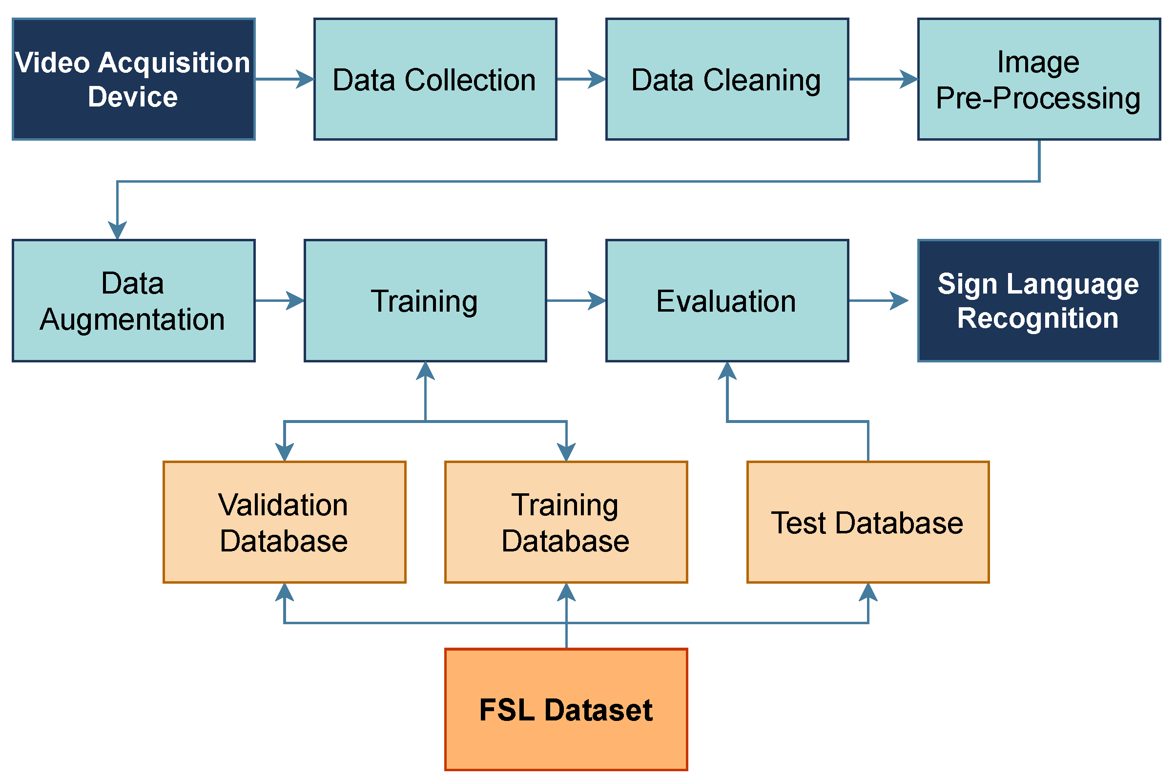
This study utilizes a video-based sign language recognition system, as shown in Figure 1. The architecture [16] involves several processes that are individually explained in the following section, including the specific techniques to be used for each process. Moreover, the system utilizes two databases: one for training the algorithm and the other for the dataset of the FSL hand signs, which serves as a benchmark for determining the expected output.

Figure 1. Adopted architecture of the vision-based Sign Language Recognition system.

3.2. System Flow

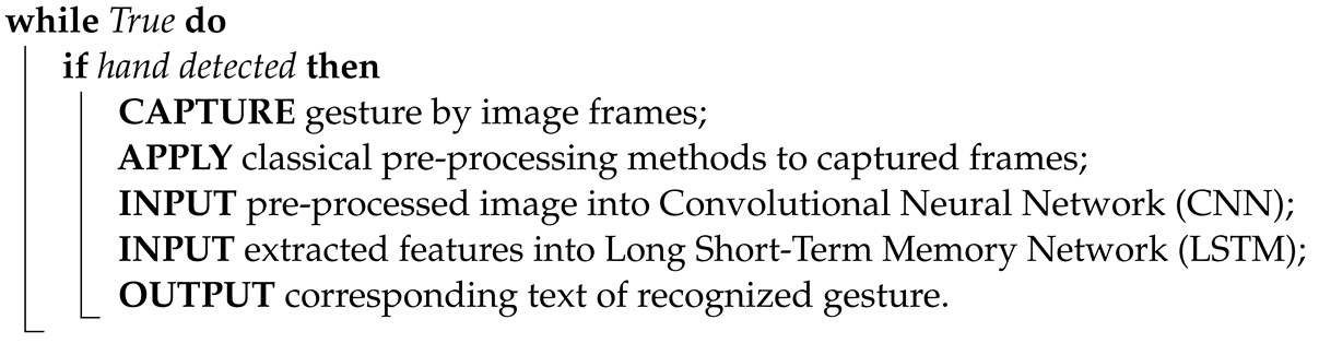
Algorithm 1 shows the overview of the proposed SLR system. It includes the techniques to be used for the following processes: Image Preprocessing, Feature Extraction, and Recognition. With that, the system is composed of a series of processes in order to identify and recognize the perceived sign from the image acquisition device.

Algorithm 1: Proposed SLR System Process.

3.3. Ethical Considerations

The study underwent an ethics review by an authorized research ethics committee, since the data collection process requires human participants. We developed our own data collection tools and a controlled setup for dataset generation. The appropriateness and fairness of the selection and recruitment of participants are critical, since the scope of the study requires knowledge of FSL. That said, the current work has collaborated with the Deaf Association in order to provide correct and accurate information on signs.

Within the research execution period, the participants visited the site for a day at their most convenient time. All participants were able to complete the data collection within a day. The main qualification of the participants was for them to be FSL signers or at least able to perform signs when taught with the proper execution. However, there were exclusions, such as minors, senior citizens, pregnant women, and people with a comorbidity, as they may have difficulty visiting the study site and fulfilling their roles as participants.

In consideration of participants’ protection, they were oriented about their roles and rights as participants and provided an overview of the study. Added to that, informed consent forms were given, which encapsulated the important details they needed to know in participating, including reimbursement for participation, confidentiality, and protection of their data. Participation in the study did not induce nor cause any form of risks/harm to the participants in the process that they underwent, as disclosed in the consent form.

3.4. Data Protection Plan

Personal information was collected solely for identification purposes and is subject to this work’s protection upheld with anonymity and confidentiality. All information pertaining to the identities of the participants, including ages and names, are kept confidential and only visible to the current work.

The participants were oriented with their roles and rights as contributors to the study and were given an overview of the study itself. They were given informed consent forms detailing reimbursement, data protection, and obligatory terms. They were given time to ask questions and go over any clarifications before signing, which served as a legal formalization of granting permission to participate in the study.

Screenshots of the signers’ recordings may be visible in the study as figures; however, the participants can opt to have their likenesses censored.

The participants are referred to by code names in the study in place of their actual names for the purpose of anonymization. Only the current work has access to the code name designation. These data are stored in hard and soft copies.

Access to the participants’ information is logged per instance with timestamps and indicated purpose for monitoring means. Additionally, computers that store the soft copies are only accessible to the current work and are encrypted with a passkey that only this work knows. They are also stored locally and encrypted to prevent unauthorized access and mitigate data loss and data theft.

The physical copies are secured inside a locked file cabinet that only this work can access. All copies are kept by the current work for a duration of two years for the purpose of the study’s validation. After that period of time, they will be shredded and fully wiped. In the event that the participants are or choose to be prematurely withdrawn from their participation in the study, their data will be wiped regardless of the time period elapsed.

Any findings acquired from the participants’ data will be shared with the participants first and further discussed before they will be made available to the public. This work shall grant them access to their test results should they request them, but only after data processing.

3.5. Data Collection and Preparation

Data collection involved capturing gestures through video recording using webcam. These recorded videos constituted the input data for processing by the neural network. The selection of 15 key gestures, as listed in Table 2, was a product of extensive consultations with members of the deaf community. These gestures were thoughtfully categorized into two distinct groups as common expressions (10) and transactional inquiries (5). The former category encompasses gestures commonly used in day-to-day conversation, while the latter pertains to typical queries encountered in transactional settings such as malls or government offices.

Table 2. List of considered FSL signs.

Common Expressions	Please	Hello	Yes	Issue
	Thank You	My name is	No	Sick
	Understand	Don’t Understand
Transactional Expressions	Payment	Where restroom	Fill-up form
	Check-up Doctor	Wait in line

Given that the study’s data comprise video recordings, unlike the still images used in related works, our approach anticipated potential variations in gesture execution speed during data collection. To address this, we standardized the speed at which signs were performed. This involved assessing video recordings of a signer executing gestures at three distinct speeds: slow, moderate, and fast. As there is no universally recognized standard for quantifying sign speed within the FSL community, these levels were determined based on the signer’s perception. The moderate speed was then adopted as the reference for gesture execution during the actual recording process.

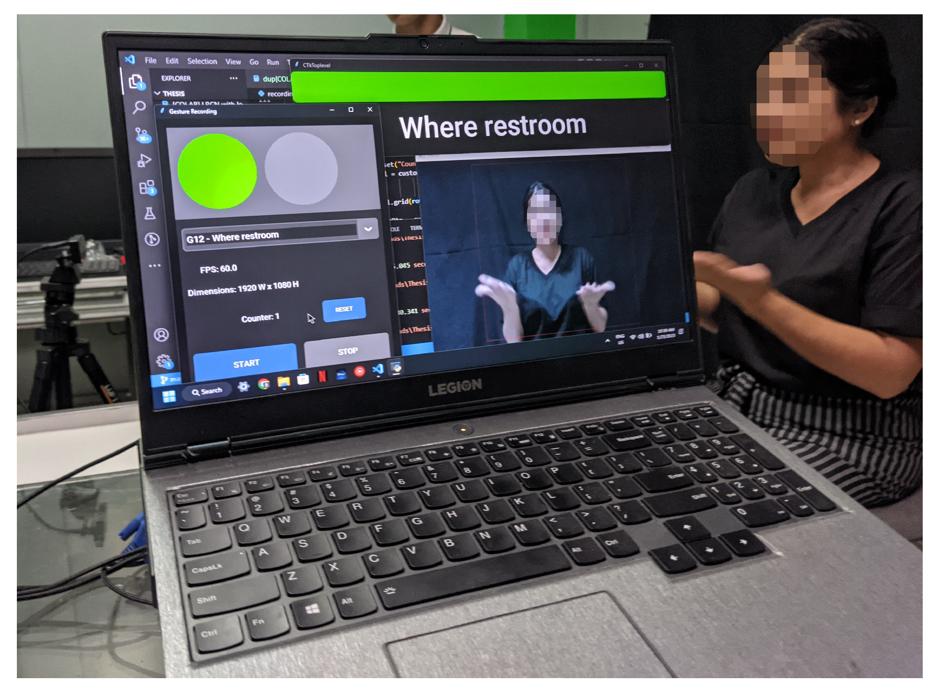
As part of the data collection procedure, the signers performed the gestures under controlled conditions, as shown in Figure 2. This ensured that the key upper body parts, including arms, head, shoulders, and chest, were precisely within a designated central area. This area was facilitated by a bounding box centered around the captured image, measuring 1156 × 866 pixels, precisely customized to meet the aforementioned conditions. By imposing such spatial restrictions, unwanted regions were effectively excluded, thereby enhancing the integrity of the dataset.

Figure 2. Data collection setup.

The 15 signs were performed by a signer. Notably, the dataset was carefully balanced, with an equal number of samples collected for each gesture. A sampling of 10 video recordings was captured for each gesture across seven different signers, culminating in a total of 1050 recordings.

For this study, we employed the ROG Eye S web camera, renowned for its exceptional specifications, with a video resolution of 1080p (1920 × 1080 pixels), image resolution of 5 megapixels, and a capture rate of 60 frames per second. These specifications were carefully selected to minimize potential noise, distortion, and delay that could impede subsequent steps in the methodology.

3.5.1. Input Image Data Preparation

Data preparation for the training of our proposed deep learning model involved crucial steps to ensure optimal model performance. Before image preprocessing, the recorded videos underwent frame cleaning. This process involved the removal of frames from the video that did not contain the signer’s hands, which was achieved through the utilization of Google MediaPipe’s sophisticated hand detection solution [30]. The rationale behind this frame cleaning step was to eliminate extraneous frames that could potentially introduce noise and adversely affect the model’s loss and accuracy during training.

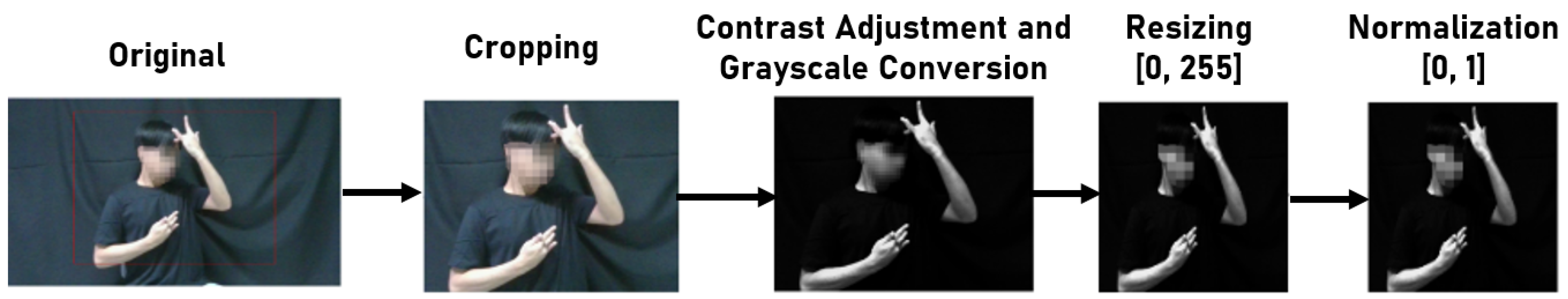
Following the frames’ removal, the resulting input image stream sequentially underwent classical image pre-processing stages, including cropping, contrast adjustment, grayscale conversion, resizing, and normalization, as presented in Figure 3. The bounding box established during data collection served as the basis for cropping the images, extracting only the region of interest for the subsequent processes. Afterwards, gamma correction was applied to enhance the contrast, followed by grayscale conversion to simplify computations. The image stream was then resized to 128 × 128 pixels, further reducing computational burden during both training and inference. This resizing ensured uniformity in input size for the deep learning model. Finally, the resized image stream underwent normalization, ensuring that all input frames had a comparable pixel distribution. This normalization step accelerated convergence during training by scaling the pixel values from the original $[0,255]$ integer range to the normalized $[0,1]$ float range [31].

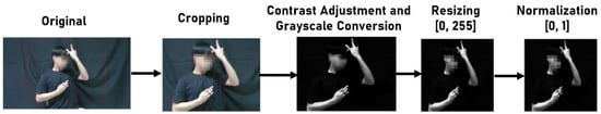
Figure 3. Adopted image preprocessing workflow.

3.5.2. Data Augmentation

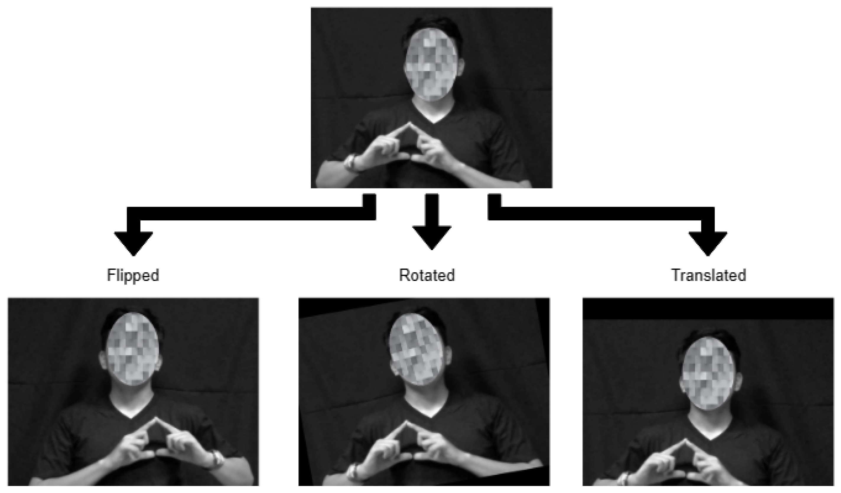
The preprocessed data were subjected to data augmentation in order to artificially expand the dataset and provide variations to enhance model performance. As illustrated in Figure 4, the augmentation procedures implemented in this study include translation, flipping, and rotation with randomized configurations. The techniques were applied for each batch of 30 frames.

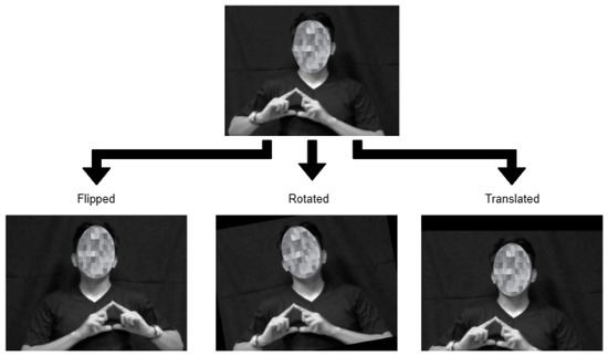
Figure 4. Illustration of the adopted data augmentation techniques.

Accordingly, a random translation moves the frame along the x-axis by between −40 and 40 pixels and along the y-axis by between −35 and 35 pixels. Only horizontal orientation was carried out for random flipping. The random rotation ranged from −10° to 10°. With augmentation, the FSL dataset increased from 1050 recordings to 21,000 after augmentation, with 1400 samples for each class.

3.6. CNN-LSTM Model

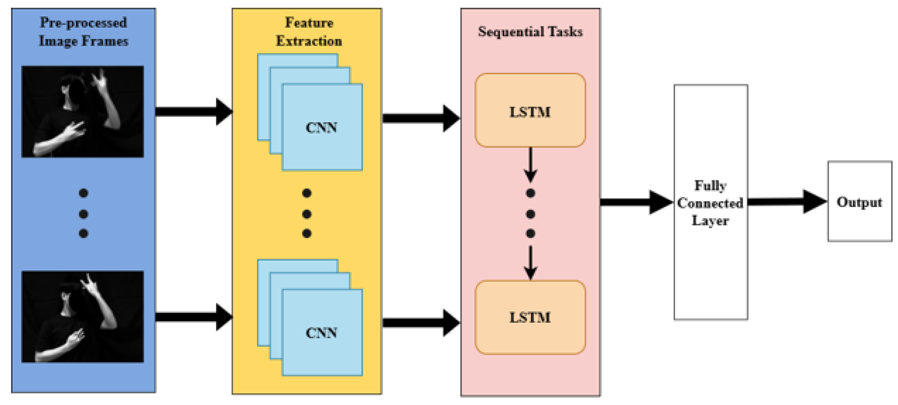
Convolutional Neural Networks (CNNs) and Long Short-Term Memory (LSTM) Recurrent Neural Networks are two cutting-edge deep learning models [32,33,34,35,36], which we combined to create the proposed model, as shown in Figure 5. CNN is in charge of extracting distinguishing or distinctive features from an input image [16]. In the CNN-LSTM framework, CNN takes a sequence of input images $X=X_1,X_2,\dots .,X_T$, where $X_t\in {\mathbb{R}}^{H\times W\times C}$ represents the image frame at time step t with height H, width W, and C channels. The feature map extraction operates by running a convolutional filter on an input image [37], as expressed in Equation (1):

$$C_t^{\left(l\right)}(i,j,k)=\sigma \left(\sum _{m=1}^{M^{\left(l\right)}}\sum _{n=1}^{N^{\left(l\right)}}{W}_{m,n,k}^{\left(l\right)}\times X_t(i+m-1,j+n-1,k)+b_k^{\left(l\right)}\right),$$

(1)

where $C_t^{\left(l\right)}$ denotes the output feature map of the l-th convolution layer at time step t, $W_{m,n,k}^{\left(l\right)}$ are the weights of the convolutional kernel, $b_k^{\left(l\right)}$ is bias term, $\sigma$ is the activation function (e.g., ReLU), and $M^{\left(l\right)}$, $N^{\left(l\right)}$ are the spatial dimensions of the kernel. Subsequently, the max pooling operation, defined in Equation (2), is applied to downscale the output feature:

$$P_t^{\left(l\right)}(i,j,k)=\underset{m,n}{max}\left(C_t^{\left(l\right)}(s·(i-1)+m,s·(j-1)+n,k)\right),$$

(2)

where $P_t^l$ represents the output of the pooling layer at time step t, s is the stride, and $\left(i,j,k\right)$ denote the spatial position and channel index.

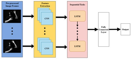
Figure 5. Simplified illustration of the CNN-LSTM model.

Meanwhile, LSTM introduces a way to capture long-term connections in sequences, making it very good at analyzing data that are arranged in chronological order. LSTM computes the hidden state $h_t$ at time step t using $h_t=LSTM(P_t,h_{t-1})$. Accordingly, the LSTM cell processes the pooled feature maps $P_t$ along with the previous hidden state $h_{t-1}$ and updates its internal state using the following composite function:

$$\begin{array}{cc}\hfill & f_t=\sigma (W_f·[h_{t-1},P_t]+b_f)\hfill \\ \hfill & i_t=\sigma (W_i·[h_{t-1},P_t]+b_i)\hfill \\ \hfill & o_t=\sigma (W_o·[h_{t-1},P_t]+b_o)\hfill \\ \hfill & {\widehat{C}}_t=tanh(W_C·[h_{t-1},P_t]+b_{{\widehat{C}}_t})\hfill \\ \hfill & C_t=f_t\odot C_{t-1}+i_t\odot {\widehat{C}}_t\hfill \\ \hfill & h_t=o_t\odot tanh\left(C_t\right),\hfill \end{array}$$

(3)

where $f_t$, $i_t$, and $o_t$ are the forget, input, and output gates, respectively, ${\widehat{C}}_t$ is the candidate cell state, $C_t$ is the updated cell state, ⊙ denotes element-wise multiplication, and $tanh$ is the hyperbolic tangent activation function.

Finally, the output of the LSTM $h_t$ is subsequently fed to the fully connected layer with softmax activation function at the output layer, as defined by the following equation:

$$\begin{array}{cc}\hfill & z=W_p·h_t+b\hfill \\ \hfill & y=W_l·z+b\hfill \\ \hfill & p_k=\frac{e^{y_k}}{{\sum }_{j=1}^K{e}^{y_j}}\mathrm{for}k=1,2,\dots ,K,\hfill \end{array}$$

(4)

where $W_p\in {\mathbb{R}}^{M\times H}$ is the weight matrix connecting the LSTM output to the fully connected layer, M is the number of neurons, H is the dimensionality of $h_t$, $W_p\in {\mathbb{R}}^{K\times M}$ is weight matrix connecting to the output layer, K is the number of target gestures, $p_k$ is the probability of the input X belonging to gesture k, $y_k$ is the k-th component of the vector y, and $b\in {\mathbb{R}}_F$ is the corresponding bias vector at layer F.

The hyperparameter values for the CNN-LSTM model were determined through empirical testing and informed by established practices and architecture found in relevant literature of the same domain. Starting with initial settings and grounded in these principles, the model underwent training using these hyperparameters. Throughout the training process, metrics such as loss and accuracy were monitored to assess the model’s learning dynamics and detect indications of underfitting or overfitting. Adjustments to the hyperparameter setting were made iteratively based on observed performance trends, aiming to achieve the preset accuracy specifically tailored to the characteristics of the dataset being used. This iterative approach ensured that the model was effective for the task at hand.

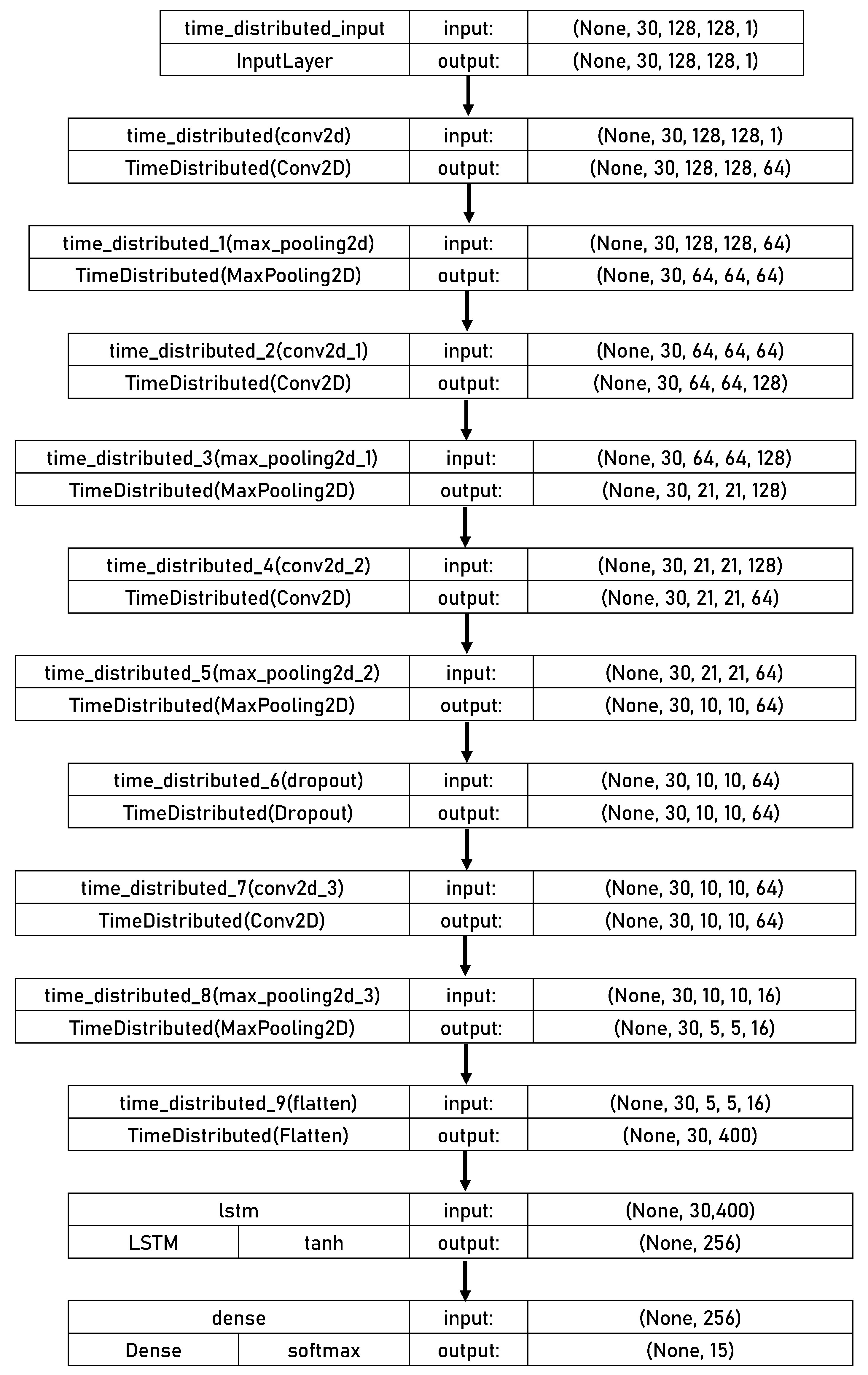
The model architecture comprises a fully-connected dense layer, 1 dropout layer, 1 LSTM layer, and 4 CNN layers. The input model shape is (30, 128, 128, 1). The Rectified Linear Unit (ReLU) was used as the activation function in all CNN layers, which all had a 3 × 3 kernel size. A MaxPooling layer with a 2 × 2 pooling window follows the initial CNN layer, which comprises 64 convolution filters. Additionally, 128 convolution filters are used in the second layer, which is followed by a 3 × 3 MaxPooling layer. Following another 2 × 2 MaxPooling layer, the third and fourth layers include 64 and 16 convolution filters. A Flatten layer is used to flatten the CNN features that have been retrieved. The LSTM network with 256 nodes, $tanh$ as its activation function, and sigmoid as its recurrent activation function receives the flattened output. Before the fourth layer, a dropout layer with a dropout rate of 0.2 is added as a regularization method that uses a random “drop-out” or node-disabling process during training to prevent overfitting. Finally, there are 15 softmax-activated nodes in the output dense layer. The CNN-LSTM model’s executive summary is shown in Figure 6.

Figure 6. Structure of the proposed CNN-LSTM model.

3.7. Training Environment

Google Colaboratory was used for model training. This is a cloud service that provides access to computational infrastructure such as memory, storage, processing power, graphics processing units (GPUs), and tensor processing units (TPUs) for applications like machine learning. The FSL dataset was divided into training, validation, and testing datasets with a split ratio of 8:1:1, and the training dataset has 16,800 or 1120 samples per class—an equal amount of samples for each class. The FSL dataset is pipelined using the TensorFlow Dataset API to enhance training efficiency. Prior to training and evaluation, the datasets are shuffled and batched. The model was trained using a batch size of 8 and 25 epochs. Callback functions were included in the training setup to aid in preventing overfitting, tracking, logging training progress, and saving checkpoints. Table 3 summarizes the training configuration.

Table 3. Summary of the adopted training configuration.

Parameters	Details
Batch Size	8
Callback Functions	EarlyStopping, TensorBoard, CSVLogger, ModelCheckpoint
Loss	Categorical Cross-entropy
Metrics	Accuracy
Optimizer	Adam

3.8. Optimization

A lightweight model was developed that was optimized to be used with low-processing power-enabled devices such as mobile phones. This work employed the Quantization method in the new model, a technique in which the weights and inputs are searched for optimal low-bit intervals. This results in an insignificant reduction in precision in the weights and inputs by making floating-point operations into integer operations [38,39], but which speeds up inferences and reduces memory utilization. There are two quantization methods. The Post-Quantization method is where the quantization application is done after extraction and training of data. The usage of dynamic range post-quantization is a good starting point, as it reduces memory utilization and speeds up calculations without requiring a representative dataset for calibration [40]. Quantization-aware training, on the other hand, involves continuous weight adjustments as it learns in order to better fit the quantization operations [39]. This training is designed to have a low error in quantized models, as it involves numerical errors being exposed and simulating them to a forward pass [41].

3.9. Testing Environment

The study used two test setups to evaluate the models on different platforms, namely, on a laptop and embedded, which utilize different architectures. The first setup is a laptop for model testing and evaluation in the x86 architecture. On the other hand, the second setup is a Raspberry Pi 4 for the ARM architecture. Additionally, both setups used the same software versions for testing in order to control software-related impact on performance. Table 4 shows the detailed hardware and software specifications of the setups.

Table 4. Hardware and software specifications.

		Hardware & Software	Details
Setup 1	Model		Lenovo IdeaPad 3 15ARE05
	CPU		AMD Ryzen 7 4700 U
	Architecture		Zen 2 (x86)
	RAM		8 GB
	OS		Windows 11 22H2
	Python		3.9.16
	Tensorflow		2.10.0
	Keras		2.10.0
Setup 2	Model		Raspberry Pi 4 Model B
	CPU		Broadcom BCM2711
	Architecture		ARMv8-A
	RAM		4 GB
	OS		Raspberry Pi OS 11 “Bullseye”
	Python		3.9.16
	Tensorflow		2.10.0
	Keras		2.10.0

4. Results and Discussion

4.1. Base Model Training History

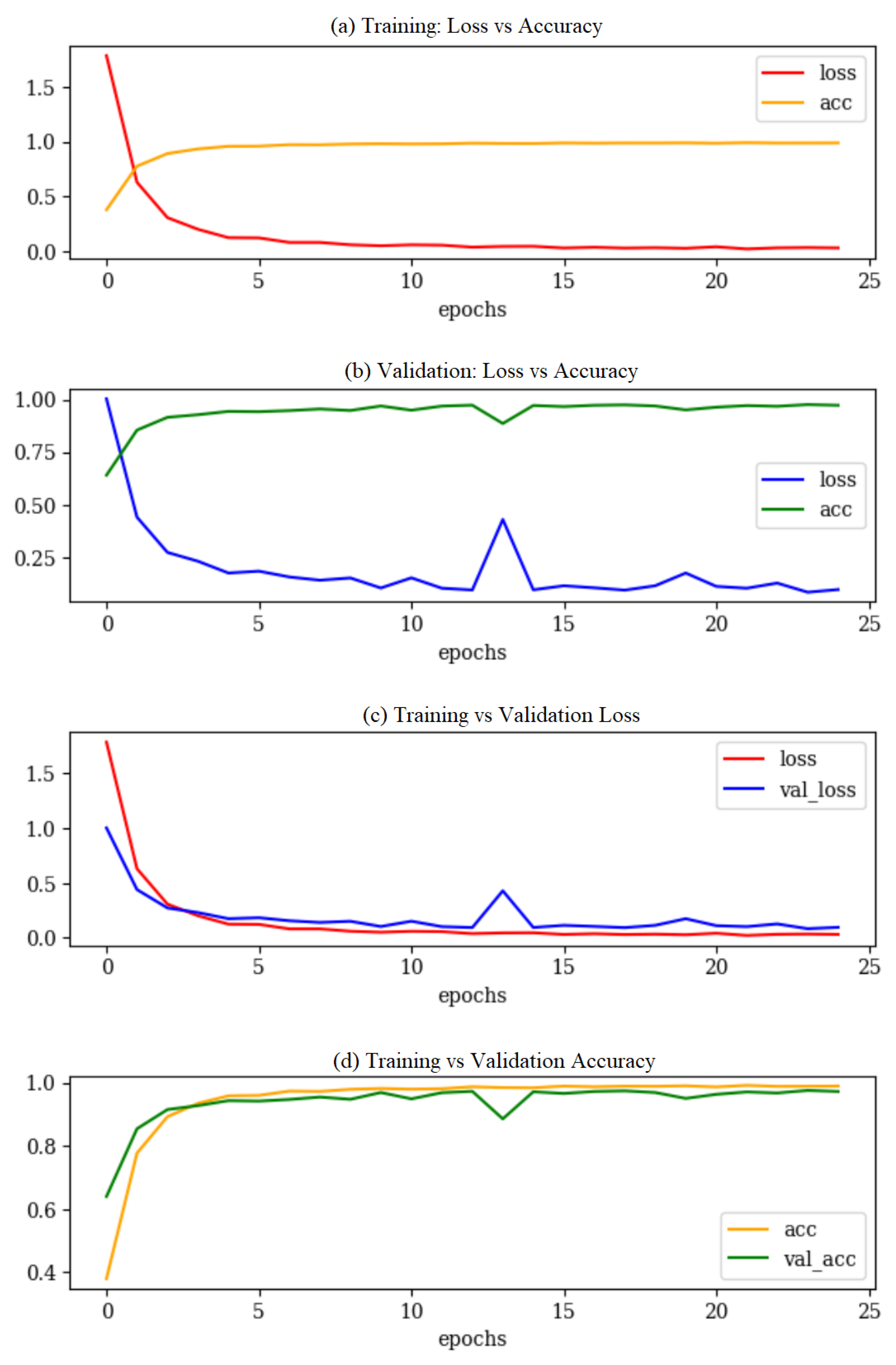
The metrics in Figure 7 demonstrate the progression of: (a) loss vs. accuracy during model training, (b) validation loss vs. validation accuracy, (c) training loss vs. validation loss, and (d) training accuracy vs. validation accuracy. The model had not undergone overfitting, meaning it was able to generalize with its functions not too closely aligned to a limited set of data points. During validation, accuracy levels peaked at the 24th epoch at 0.976. It can be observed that there was a noticeable drop in the validation accuracy at the 14th epoch. The training gradient momentum that is built up over a few mini-batches may work very well for a while until it hits a mini-batch that requires the model to learn something different, which explains this sudden spike in validation loss. The overall model was able to reach similar accuracy levels during validation, implying that it was well-fit with unseen data.

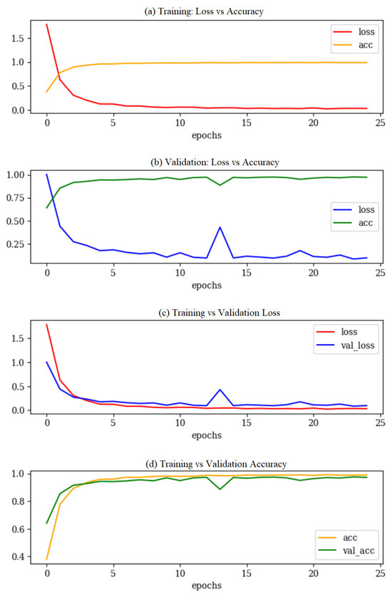
Figure 7. Comparison of training and validation performance.

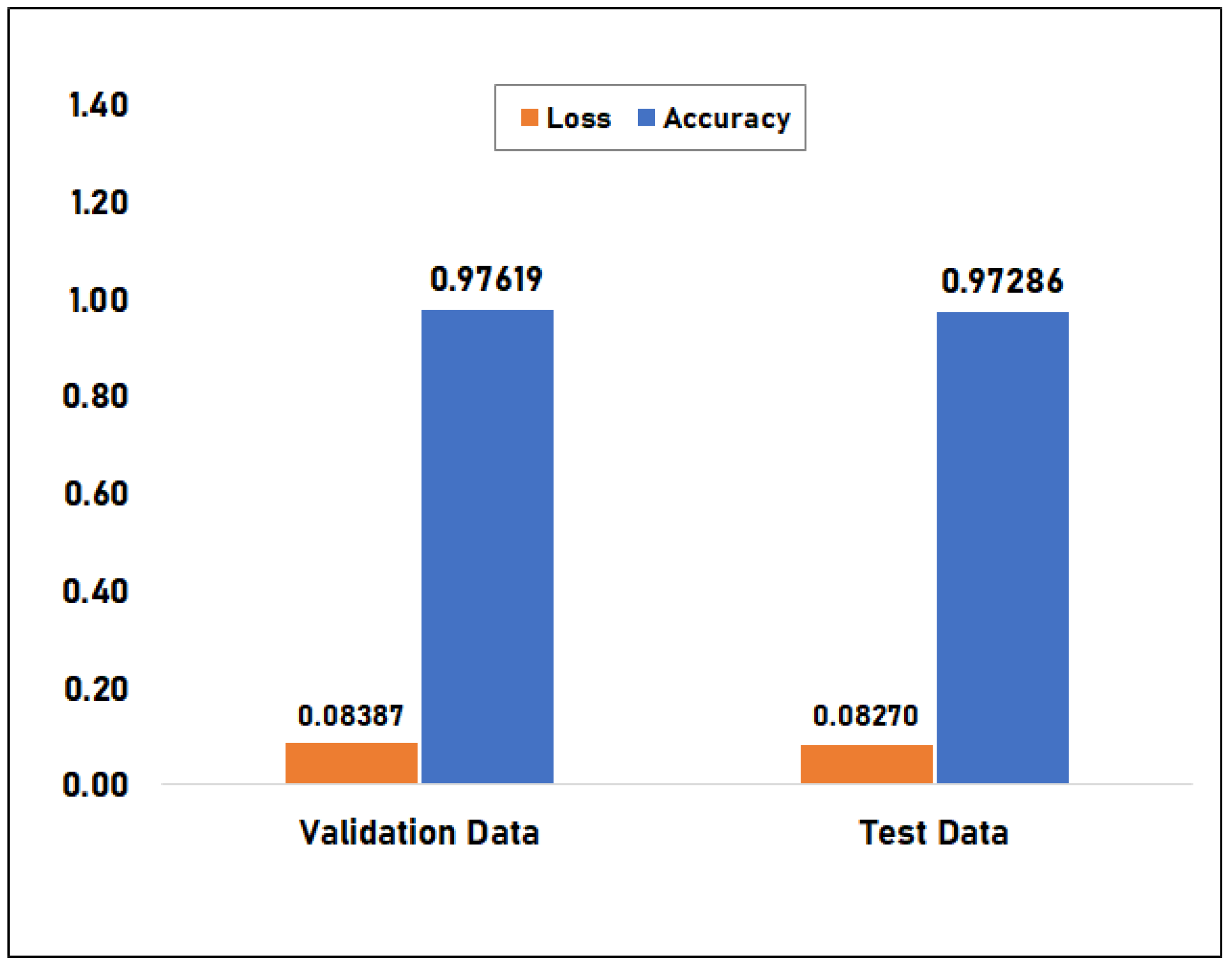
Figure 8 compares the accuracy and loss of the base CNN-LSTM model using test and validation data. Both datasets comprise 2100 samples for evaluating the loss and accuracy of the model on unseen data. On validation data, the base model has a 97.619% accuracy rate and a 0.084 loss. The model’s accuracy on test data was 97.286%, which is insignificantly less than the accuracy during validation. The test loss of 0.083 is the same case. The results imply that the model is well-fit with unseen data and that it was successful in generalizing the features while being trained.

Figure 8. Accuracy comparison between test data versus validation data for the Base Model.

4.2. Model Size

Figure 9 shows the model sizes of the base model and the quantized models. The base model had a size of 9843.880 KB. Lightweight model 1 had a size of 842.102 KB, which is 92% less than the base model, while lightweight model 2 had a size of 3278.390 KB, which is 66% less than the base model. Among the three models, the base model had the largest size, while lightweight model 1 had the smallest.

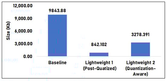
Figure 9. Model size comparison between the base model versus lightweight versions.

Results imply that the quantization method reduces the model size of the base model. There is also a noticeable difference between the post-quantization and quantization-aware processes. This difference is due to the post-quantization process of the whole model making it much smaller, compared to the quantization-aware. In that model, critical layers are not quantized directly, meaning only selected layers can be quantized, reducing only a portion of the model.

4.3. Classification Evaluation

Every gesture in the model was labeled as one of the four outcomes through the confusion matrix. One is a true positive (TP), wherein the model properly predicts the positive class. A true negative (TN) is the result where the model properly predicts the negative class. A false positive (FP) is the result where the model incorrectly predicts the positive class, and a false negative (FN) is the result where the model incorrectly predicts the negative class.

When classifying Gesture 0 (Check-up Doctor) as an example, the resulting values of the outcome metrics are as follows:

$$\begin{array}{cc}\hfill TP& =140,\hfill \\ \hfill FN& =2,\hfill \\ \hfill FP& =2,\hfill \\ \hfill TN& =1956.\hfill \end{array}$$

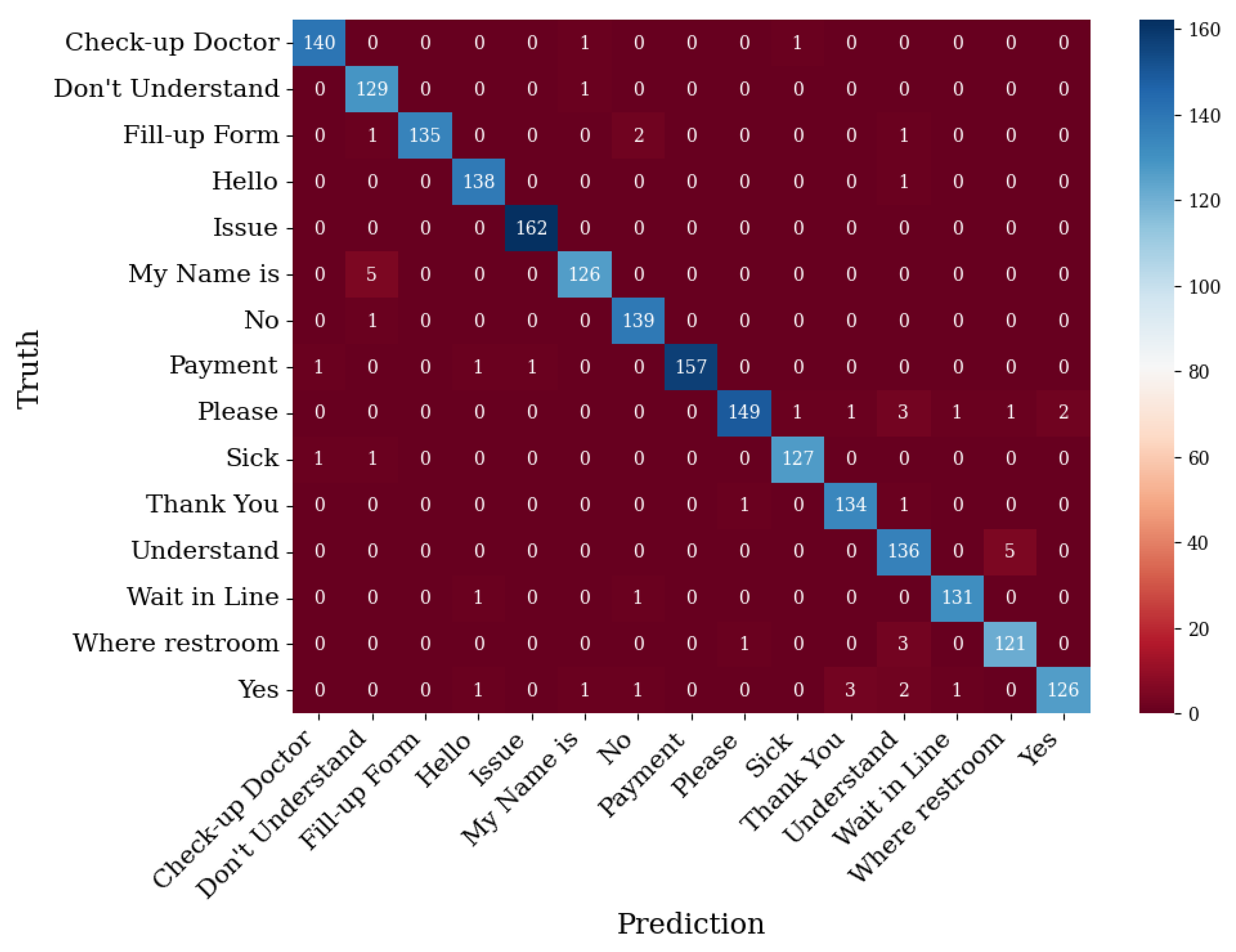
The confusion matrix in Figure 10 shows that there were gestures that were misclassified by the system. The gesture that saw no problems in the detection was the gesture Issue, with 162 as its true positive label and 0 as its false positive and false negative labels. On the other hand, the gesture that had a high misclassification rate was Where Restroom, where its true positive label was 121, with 6 and 4 for its false positive and false negative labels, respectively.

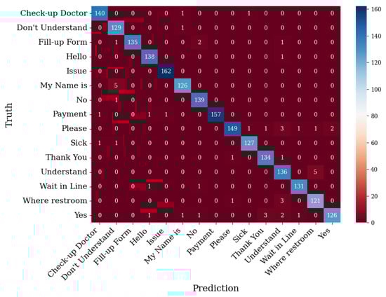
Figure 10. Validation data confusion matrix for base model.

Once the values of these outcomes were recorded, the accuracy level was defined as the ratio between the number of correct predictions and the total number of predictions. The precision level was defined as the ratio between the number of Positive samples correctly classified and the total number of samples classified as Positive (either correctly or incorrectly). Meanwhile, the recall level was defined as the proportion of Positive samples that were accurately categorized as Positive to the total number of Positive samples. Lastly, the F1-score was defined as the arithmetic mean of the precision and recall values.

Table 5 summarizes the precision, recall, F1-score, and support values for each gesture and their respective accuracy levels, macro-averages, and weighted averages. Support is defined as the number of ground truth occurrences of each class. The macro-averages were calculated by averaging the unweighted mean per label and the weighted averages by averaging the support-weighted mean per label. Based on the table, most of the values of the F1-score were around 0.98 to 1.00, implying that the two gestures have near-perfect precision and recall, implying that the model overall has a high classification rate of distinguishing between gestures.

Table 5. Classification metrics summary.

Class	Precision	Recall	F1-Score	Support
0 (Check-up Doctor)	0.99	0.99	0.99	142
1 (Don’t Understand)	0.94	0.99	0.97	130
2 (Fill-up Form)	1.00	0.97	0.99	139
3 (Hello)	0.98	0.99	0.99	139
4 (Issue)	0.99	1.00	1.00	162
5 (My Name is)	0.98	0.96	0.97	131
6 (No)	0.97	0.99	0.98	140
7 (Payment)	1.00	0.98	0.99	160
8 (Please)	0.99	0.94	0.96	158
9 (Sick)	0.98	0.98	0.98	129
10 (Thank You)	0.97	0.99	0.98	136
11 (Understand)	0.93	0.96	0.94	141
12 (Wait in Line)	0.98	0.98	0.98	133
13 (Where restroom)	0.95	0.97	0.96	125
14 (Yes)	0.98	0.93	0.96	135
accuracy			0.98	2100
macro avg	0.98	0.98	0.98	2100
weighted avg	0.98	0.98	0.98	2100

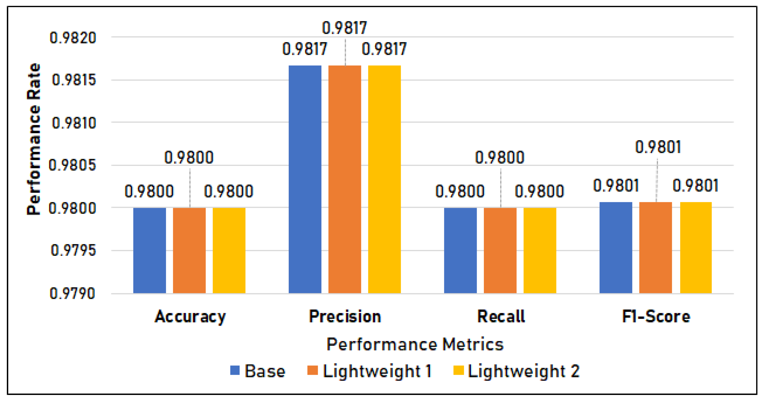
Figure 11 shows the classification metrics of the three models. It shows that there is no difference in the classification metrics, with the models having an accuracy, precision, recall, and F1-score of 0.98.

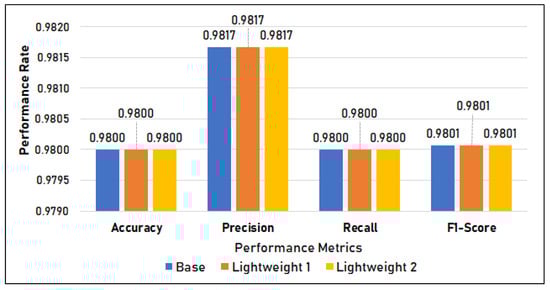
Figure 11. Classification Metrics in Setup 1.

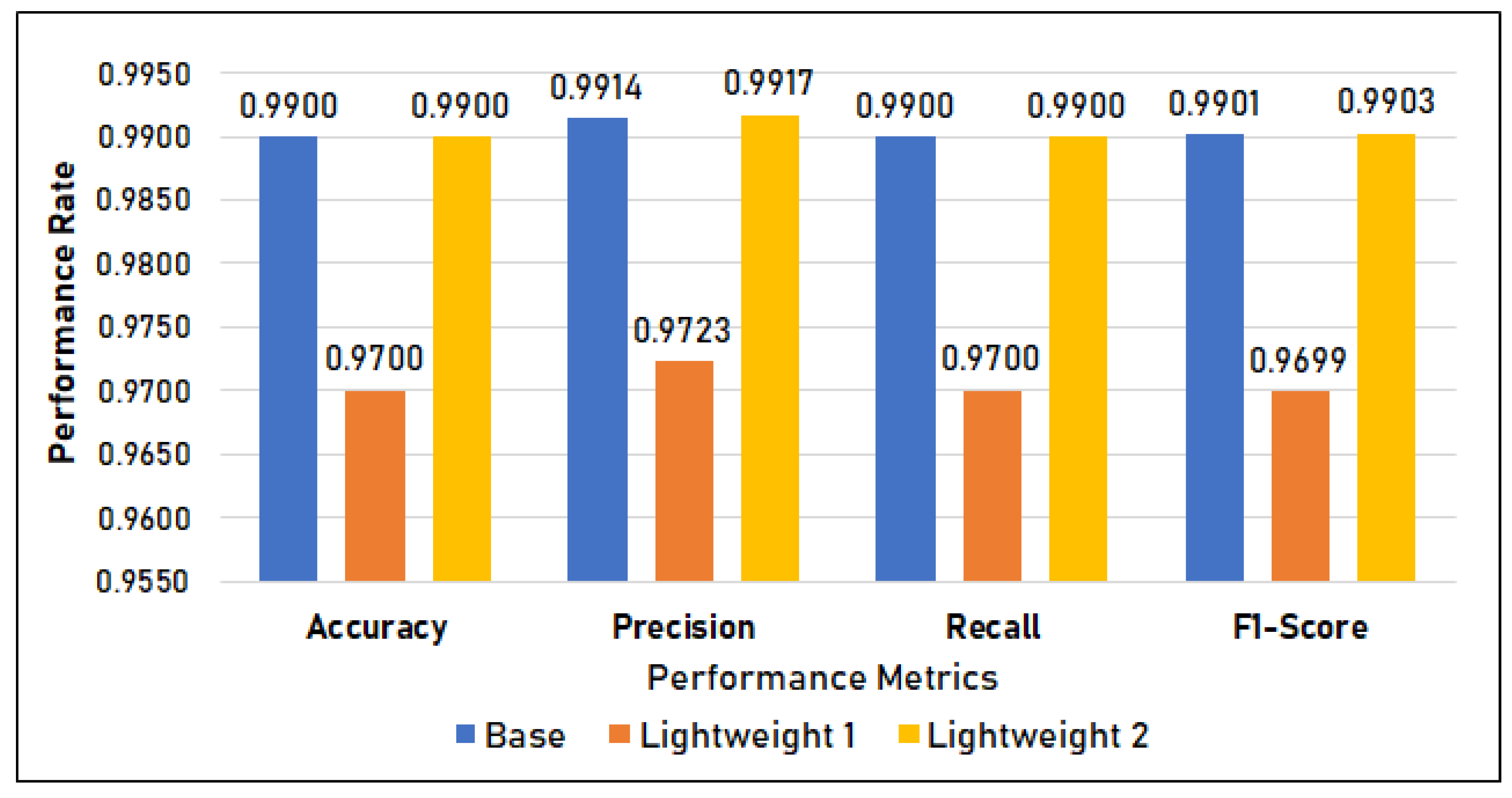
Figure 12 shows the classification metrics of the three models. It shows that there is a difference in the Post-Quantized (PQ) model’s (lightweight model classification metrics, with the models having an accuracy, precision, recall, and F1-score of 97%. On the other hand, both the base model and the lightweight model 2 scored 99%.

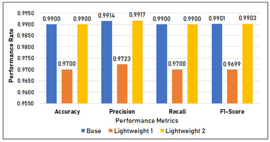
Figure 12. Classification metrics in Setup 2.

4.4. Inference Time

The data used for inference time are a subset of the validation data. For this test, 100 samples from the validation dataset were randomly selected as input for measuring the time duration of model inference. Additionally, the inference time is measured per input, and then the minimum, mean, and maximum times are computed.

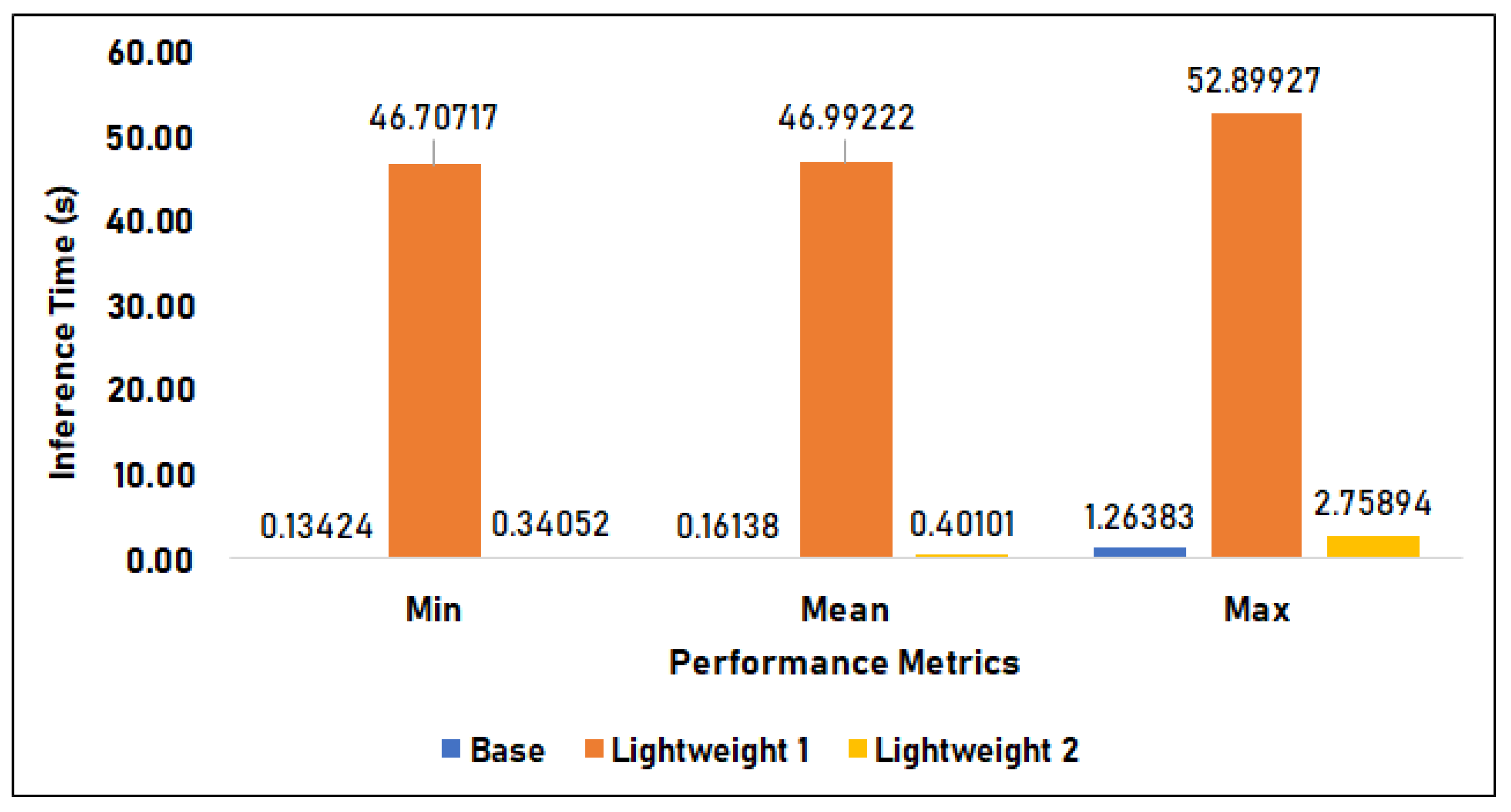
Figure 13 compares the time duration of the base model, lightweight model 1, and lightweight model 2 in Setup 1 or the x86 laptop machine environment. The base model has an average of 0.161 s inference time, a minimum time of 0.134 s, and a maximum of 0.134 s. Lightweight model 1, applied with Post-Quantization, has an inference time of 46.992 s on average, 46.707 s minimum, and 52.899 s maximum. Lastly, lightweight model 2 with Quantization-Aware Training (QAT) has a 0.401 s mean, 0.341 s minimum, and 2.759 s maximum inference time. In this setup, the base model performs the best in terms of speed, as it has the fastest minimum, mean, and maximum inference time. On the other hand, the lightweight 1 model performed the worst, as it has the slowest minimum, mean, and maximum inference time. The results of the lightweight models are slower by 1.540% on minimum, 1.480% on mean, and 1.180% on max time compared to that of the base model.

Figure 13. Inference Time in Setup 1.

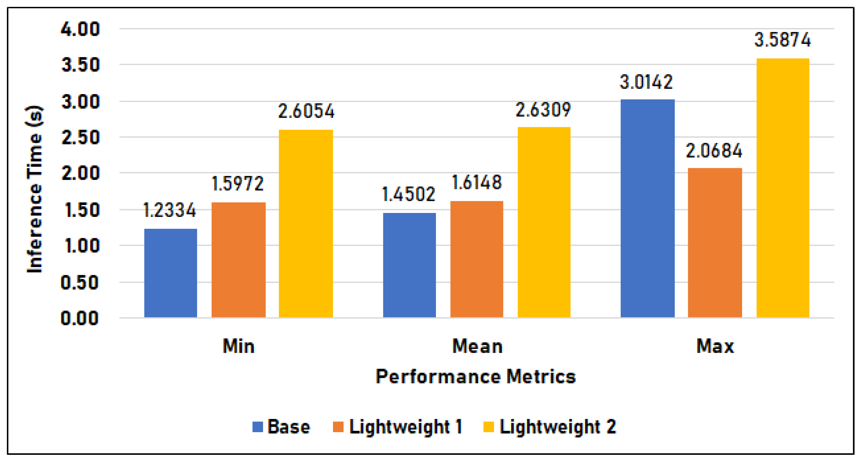
Figure 14 compares the time duration of the base model, lightweight model 1, and lightweight model 2 in Setup 2, or the Raspberry Pi setup. The base model has an average of 1.450 s inference time, a minimum time of 1.233 s, and a maximum of 3.014 s. Lightweight model 1 has an inference time of 1.615 s on average, 1.597 s minimum, and 2.068 s maximum. Lastly, lightweight model 2 has a 2.631 s mean, 2.605 s minimum, and 3.587 s maximum inference time. In this setup, the base model has the fastest minimum and mean inference but has the second-highest maximum time. In contrast, lightweight 1 (LW 1) has the lowest maximum inference time of 2.068 s and follows the base model in terms of minimum and mean inference times of 1.597 s and 1.615 s, respectively. Furthermore, lightweight 2 (LW2) has the slowest overall inference time in this setup, with 2.631 s mean, 2.605 s minimum, and 3.587 s maximum.

Figure 14. Inference time in Setup 2.

4.5. Memory Utilization

This testing uses the same sampling technique in the previous subsection, namely, a random selection of 100 samples from the validation dataset. Similar to how inference time was measured, the memory utilization per inference is traced, and then the minimum, mean, and the maximum are computed.

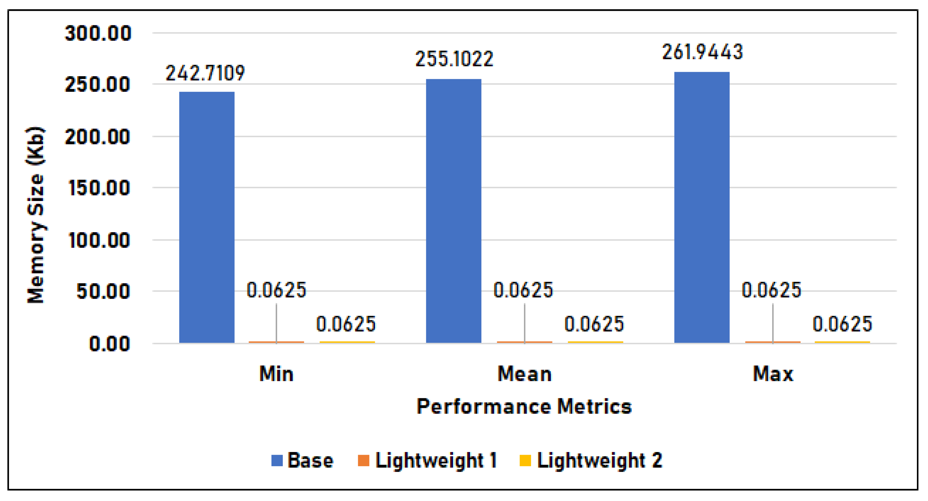
Figure 15 compares the memory utilization per inference of the base model, lightweight model 1, and lightweight model 2 in Setup 1, measured in kilobytes. Among the three models, the base model used the largest memory per inference, with an average of 255.102 KB, a minimum of 242.711 KB, and a maximum of 261.944 KB. The two lightweight models, on the other hand, utilized the same amount of memory—only 0.063 KB—across their minimum, mean, and maximum utilization. This is around 255 KB less than the base model uses.

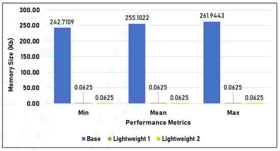
Figure 15. Memory utilization during inference in Setup 1.

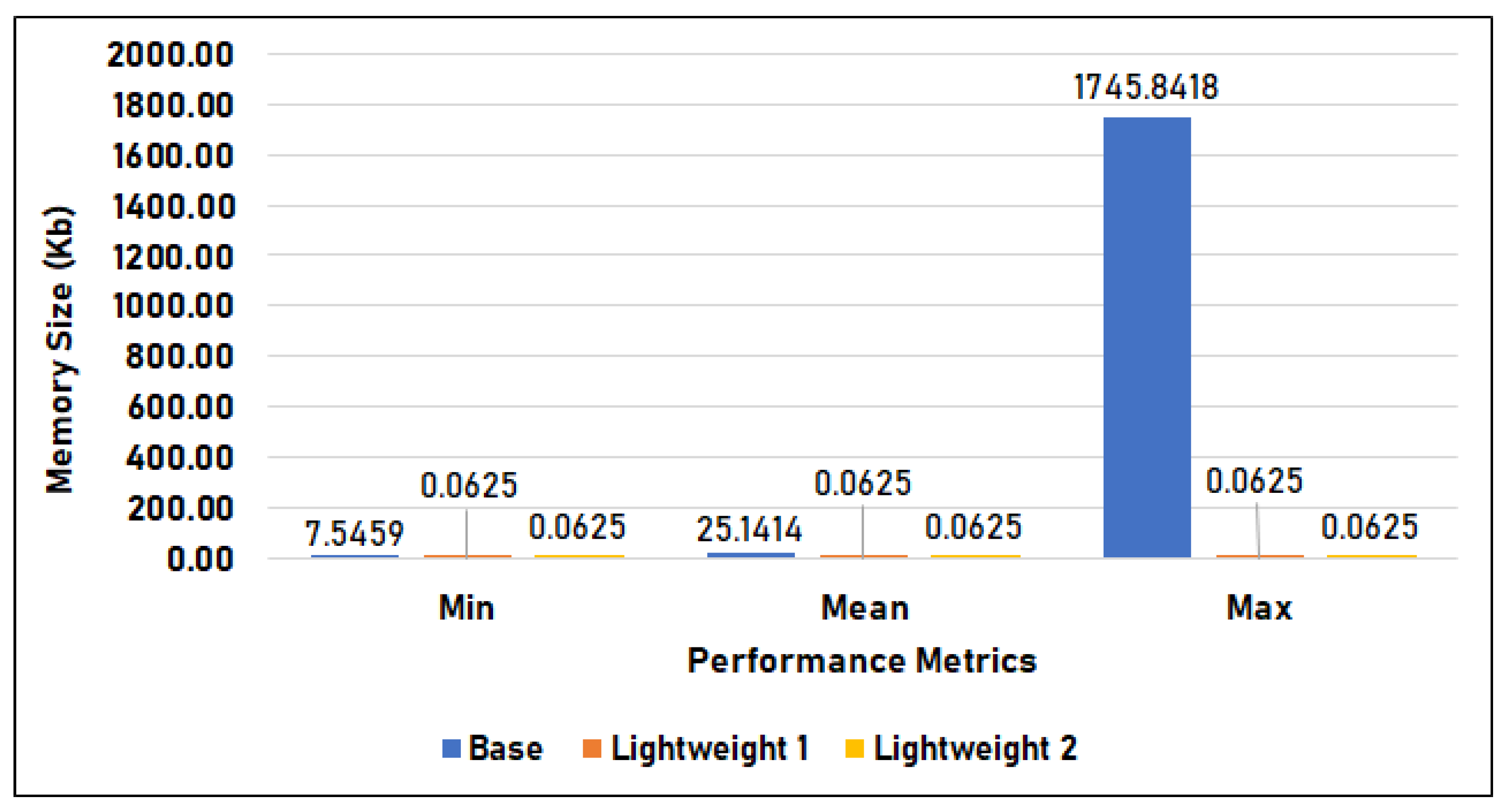
Figure 16 compares the memory utilization per inference of the base model, lightweight model 1, and lightweight model 2 in Setup 2, measured in kilobytes. Similar to the previous results in Setup 1, the base model used the largest amount of memory, with 7.546 KB minimum usage and 25.141 KB average, which is 9.15% smaller than in Setup 1, and a maximum utilization that spiked to 1745.840 KB. The memory utilization of the two lightweight models is 0.063 KB across minimum, mean, and maximum, which is consistent with the results of Setup 1.

Figure 16. Memory utilization during inference in Setup 2.

4.6. Results Summary

Table 6 summarizes the results of the previous subsections in terms of model size, classification evaluation, average inference time, and average memory utilization. The summary is divided according to the setups in which the models were evaluated and tested.

Table 6. Performance summary of the models in different setups and other works.

Setup 1 (Laptop with x86 CPU)
	Descr	Classification Metrics				Average Inference Time (s)	Average Memory Utilization (KB)	Model Size (KB)
		Accuracy	Precision	Recall	F1-Score
Base	CNN-LSTM	0.980	0.982	0.980	0.980	0.161	255.102	9843.883
LW 1	PQ	0.980	0.982	0.980	0.980	46.992	0.063	842.102
LW 2	QAT	0.980	0.982	0.980	0.980	0.401	0.063	3278.391
Setup 2 (Raspberry Pi with ARM CPU)
Model	Descr	Classification Metrics				Average Inference Time (s)	Average Memory Utilization (KB)	Model Size (KB)
		Accuracy	Precision	Recall	F1-Score
Base	CNN-LSTM	0.990	0.991	0.990	0.990	1.450	25.141	9843.883
LW 1	PQ	0.970	0.972	0.970	0.970	1.615	0.063	842.102
LW 2	QAT	0.990	0.992	0.990	0.990	2.631	0.063	3278.391
Comparison with Other Works
Ref #	Descr	Classification Metrics				Average Inference Time (s)	Average Memory Utilization (KB)	Model Size (KB)
		Accuracy	Precision	Recall	F1-Score
[11]	ResNet	0.867	—	—	—	—	—	—
[12]	CNN	0.950	—	—	—	—	—	—

The classification metrics results in Table 6 can be attributed to the Post-Quantization process applied to the whole model, in that all its layers are quantized, and the critical layers on the time-distributed and Long Short-Term Memory layers are affected, reducing its attributed classification metrics [42,43]. Meanwhile, the Quantization-Aware process that recommends not quantizing the critical layers results in quantizing only selected layers, specifically, the Dense layers, which are only a minor portion of the entire CNN-LSTM model, making its accuracy similar to that of the base model [44].

The inference time results show that the base model performs the fastest in terms of inference among the three models. This can be attributed to the fact that the TensorFlow build used in this setup is for x86/x64 processors, where the execution of the base model is optimized. Nevertheless, as a drawback, the base model’s performance became slower by 7.99% in terms of average time in Setup 2. Lightweight models 1 and 2 were both converted from the base model using TensorFlow Lite, which supposedly optimized them for the ARM instruction set for faster execution [45]. However, this is only evident with the Post-Quantized model, lightweight 1, with its improved mean inference time in Setup 2 of 28%; however, this is not the case for lightweight 2, which became slower by 5.56% in the same setup. This is due to quantizing only selected layers for Quantization-Aware training [44], specifically the Dense layers, which are only a minor portion of the entire CNN-LSTM model. Hence, the lightweight 2 model has only a few optimizations for Setup 2, and the majority of its weights and activations still have the same level of precision as the base model.

The overall results of the memory utilization test show that the base model is the most memory-intensive model, which is not ideal for devices that have limited memory capacity, such as the Raspberry Pi and mobile devices. This is different than the two lightweight models’ memory utilization, which only uses less than a kilobyte per inference. Furthermore, the results show that optimizing the base model with TensorFlow Lite greatly impacts the model’s memory usage [45].

From the given results, it can be summarized that different versions of the proposed CNN-LSTM model are more appropriate to deploy than the others depending on the setups or environments. The base model provides the best possible accuracy and fastest inference speed. This model is highly applicable to desktops and laptops, as these machines do not typically have concerns with limited memory and storage resources. On the other hand, if the aforementioned resources are to be taken into consideration, particularly in embedded devices, the lightweight 1 model or the Post-Quantized model is appropriate, since it minimizes both model size and inference memory utilization with minimal impact on accuracy. Additionally, the inference speed of this model is comparable to the base model when executed on devices with limited resources, as seen in Table 6. The lightweight 2 Quantization-Aware model can be used as an alternative for the base model, as it has an advantage in terms of memory utilization and model size but comparable accuracy, with a compromise on slower inference speed compared to the base model.

Finally, Table 6 also presents a comparison of the proposed CNN-LSTM model with other existing works focusing on FSL gesture recognition. Our model outperforms previous approaches, achieving an accuracy improvement of 11.3% and 3.0% compared to [11,12], respectively.

5. Conclusions

This work proposed a gesture recognition system for Filipino Sign Language using Convolutional and Long Short-Term Memory Neural Networks. Based on the metrics and test results, the CNN-LSTM model was able to recognize the given FSL signs involving movements with relatively high precision. Accuracy, precision, recall, and F1-score were used to evaluate the performance of the suggested model. The model was able to obtain 98% in the classification metrics. Additionally, the accuracy and loss of the model were comparable for the validation and test sets of data: 97.62% accuracy and 0.0839 loss for the validation set, and 97.29% accuracy and 0.0827 loss for the test set, implying it is well-fit with its features successfully generalized. The model underwent the Post-Quantization process and Quantization-Aware training to develop lightweight models meant for resource-constrained devices.

In addition to the classification metrics, the average inference time and memory utilization of the three models were also tested in ARM-based and x86-based setups. The base model showed the largest size at 9843.88 KB, while lightweight model 1 had the lowest at 842.11 KB, which is 92% less than the base model. Across the two setups, the base model was consistently the most accurate and fastest in inference time but also had the largest model size and memory utilization. In Setup 1, results showed identical classification metrics across the three models; however, lightweight model 1 had a significantly higher inference time that could be attributed to the whole model and all its layers becoming quantized after training. In Setup 2, the same reason also reduced the classification metrics for lightweight model 1, albeit only by an insignificant margin. However, inference time improved for lightweight model 1, only bested by the base model. Lightweight model 2 in the ARM-based setup had the longest inference time, roughly 1 s more than the other models.

Based on the results, all three models demonstrated high accuracy levels and low loss levels, making them capable of converting FSL gestures in real-time and usable for digital applications and dedicated hardware such as in government service centers and banks. However, the data also showed that different models of the proposed CNN-LSTM implementation are more appropriate to be deployed and used than others, depending on the environment and devices available. As part of future work aimed at enhancing the robustness and applicability of the proposed model in diverse real-world scenarios, we will conduct a comprehensive ablation study to systematically analyze the impact of various model components.

References

- World Health Organization. Deafness and Hearing Loss. 2021. Available online: https://www.who.int/news-room/fact-sheets/detail/deafness-and-hearing-loss (accessed on 28 October 2021).
- Nearly One in Six in the Philippines Has Serious Hearing Problems. 2021. Available online: https://hearingyou.org/news/nearly-one-in-six-in-the-philippines-has-serious-hearing-problems/ (accessed on 28 October 2021).
- Newall, J.P.; Martinez, N.; Swanepoel, D.W.; McMahon, C.M. A national survey of hearing loss in the Philippines. Asia Pac. J. Public Health 2020, 32, 235–241. [Google Scholar] [CrossRef] [PubMed]
- Maria Feona Imperial. Kinds of Sign Language in the Philippines. 2015. Available online: https://verafiles.org/articles/kinds-of-sign-language-in-the-philippines (accessed on 28 October 2021).
- Mendoza, A. The Sign Language Unique to Deaf Filipinos. 2018. Available online: https://web.archive.org/web/20221010011356/cnnphilippines.com/life/culture/2018/10/29/Filipino-Sign-Language.html (accessed on 29 October 2021).
- RA 11106—An Act Declaring the Filipino Sign Language as the National Sign Language of the Filipino Deaf and the Official Sign Language of Government in All Transactions Involving the Deaf, and Mandating Its Use in Schools, Broadcast Media, and Workplaces. 2018. Available online: https://www.ncda.gov.ph/disability-laws/republic-acts/ra-11106/ (accessed on 28 October 2021).
- Resources for the Blind, Inc.—Philippines. GABAY (Guide): Strengthening Inclusive Education for Blind, Deaf and Deafblind Children. 2021. Available online: https://www.edu-links.org/sites/default/files/media/file/CIES%202021%20Gabay%20Presentation.pdf (accessed on 30 October 2021).
- Butler, C. Signs of Inclusion. USAID Supports Creation of Filipino Sign Language Dictionary and Curriculum. 2021. Available online: https://medium.com/usaid-2030/signs-of-inclusion-5d78d91bce51 (accessed on 29 October 2021).
- Rivera, J.P.; Ong, C. Facial expression recognition in filipino sign language: Classification using 3D Animation units. In Proceedings of the 18th Philippine Computing Science Congress (PCSC 2018), Cagayan de Oro, Philippines, 15–17 March 2018; pp. 1–8. [Google Scholar]
- Cabalfin, E.P.; Martinez, L.B.; Guevara, R.C.L.; Naval, P.C. Filipino sign language recognition using manifold projection learning. In Proceedings of the TENCON 2012 IEEE Region 10 Conference, Cebu, Philippines, 19–22 November 2012; IEEE: Piscataway, NJ, USA, 2012; pp. 1–5. [Google Scholar]
- Montefalcon, M.D.; Padilla, J.R.; Llabanes Rodriguez, R. Filipino Sign Language Recognition Using Deep Learning. In Proceedings of the 2021 5th International Conference on E-Society, E-Education and E-Technology, Taipei, Taiwan, 21–23 August 2021; Association for Computing Machinery: New York, NY, USA, 2021; pp. 219–225. [Google Scholar]
- Jarabese, M.B.D.; Marzan, C.S.; Boado, J.Q.; Lopez, R.R.M.F.; Ofiana, L.G.B.; Pilarca, K.J.P. Sign to Speech Convolutional Neural Network-Based Filipino Sign Language Hand Gesture Recognition System. In Proceedings of the 2021 International Symposium on Computer Science and Intelligent Controls (ISCSIC), Rome, Italy, 12–14 November 2021; pp. 147–153. [Google Scholar] [CrossRef]
- Kishore, P.; Kumar, P.R. A video based Indian sign language recognition system (INSLR) using wavelet transform and fuzzy logic. Int. J. Eng. Technol. 2012, 4, 537–542. [Google Scholar] [CrossRef]
- Tolentino, L.K.S.; Juan, R.S.; Thio-ac, A.C.; Pamahoy, M.A.B.; Forteza, J.R.R.; Garcia, X.J.O. Static sign language recognition using deep learning. Int. J. Mach. Learn. Comput. 2019, 9, 821–827. [Google Scholar] [CrossRef]
- Ong, C.; Lim, I.; Lu, J.; Ng, C.; Ong, T. Sign-language recognition through gesture & movement analysis (SIGMA). In Mechatronics and Machine Vision in Practice 3; Springer: Cham, Switzerland, 2018; pp. 235–245. [Google Scholar]
- Adeyanju, I.; Bello, O.; Adegboye, M. Machine learning methods for sign language recognition: A critical review and analysis. Intell. Syst. Appl. 2021, 12, 200056. [Google Scholar] [CrossRef]
- Pansare, J.; Gawande, S.; Ingle, M. Real-Time Static Hand Gesture Recognition for American Sign Language (ASL) in Complex Background. J. Signal Inf. Process. 2012, 3, 364–367. [Google Scholar] [CrossRef]
- Islam, M.M.; Siddiqua, S.; Afnan, J. Real time Hand Gesture Recognition using different algorithms based on American Sign Language. In Proceedings of the 2017 IEEE International Conference on Imaging, Vision & Pattern Recognition (icIVPR), Dhaka, Bangladesh, 13–14 February 2017; pp. 1–6. [Google Scholar] [CrossRef]
- Sia, J.C.; Cronin, K.; Ducusin, R.; Tuaño, C.; Rivera, P. The Use of Motion Sensing to Recognize Filipino Sign Language Movements; De La Salle University: Manila, Philippines, 2019. [Google Scholar] [CrossRef]
- Burns, E. What Is Machine Learning and Why Is It Important? 2021. Available online: https://searchenterpriseai.techtarget.com/definition/machine-learning-ML (accessed on 5 November 2021).
- Murillo, S.C.M.; Villanueva, M.C.A.E.; Tamayo, K.I.M.; Apolinario, M.J.V.; Lopez, M.J.D.; Edd. Speak the Sign: A Real-Time Sign Language to Text Converter Application for Basic Filipino Words and Phrases. Cent. Asian J. Math. Theory Comput. Sci. 2021, 2, 1–8. [Google Scholar]
- Yasrab, R.; Gu, N.; Zhang, X. An Encoder-Decoder Based Convolution Neural Network (CNN) for Future Advanced Driver Assistance System (ADAS). Appl. Sci. 2017, 7, 312. [Google Scholar] [CrossRef]
- What is Long Short-Term Memory (LSTM)? Available online: https://algoscale.com/blog/what-is-long-short-term-memory-lstm/ (accessed on 30 April 2021).
- Brownlee, J. CNN Long Short-Term Memory Networks. 2017. Available online: https://machinelearningmastery.com/author/jasonb/ (accessed on 30 April 2021).
- Tiongson, P.V.; Martinez, L. Initiatives for Dialogue. In Full Access: A Compendium on Sign Language Advocacy and Access of the Deaf to the Legal System; Initiatives for Dialogue and Empowerment through Alternative Legal Services (IDEALS), Inc.: Quezon City, Philippines, 2007. [Google Scholar]
- Abat, R.; Martinez, L.B. The history of sign language in the Philippines: Piecing together the puzzle. In Proceedings of the 9th Philippine Linguistics Congress: Proceedings, Quezon City, Philippines, 25–27 January 2006. [Google Scholar]
- Andrada, J.; Domingo, R. Key Findings for Language Planning from the National Sign Language Committee (Status Report on the Use of Sign Language in the Philippines). In Proceedings of the 9th Philippine Linguistics Congress: Proceedings, Quezon City, Philippines, 25–27 January 2006. [Google Scholar]
- Philippine Deaf Research Center; Philippine Federation of the Deaf. An Introduction to Filipino Sign Language; Philippine Deaf Resource Center: Quezon City, Philippines, 2004. [Google Scholar]
- Ong, S.C.; Ranganath, S. Automatic sign language analysis: A survey and the future beyond lexical meaning. IEEE Trans. Pattern Anal. Mach. Intell. 2005, 27, 873–891. [Google Scholar] [CrossRef] [PubMed]
- Vakunov, A.; Chang, C.L.; Zhang, F.; Sung, G.; Grundmann, M.; Bazarevsky, V. MediaPipe Hands: On-Device Real-Time Hand Tracking. 2020. Available online: https://mixedreality.cs.cornell.edu/workshop (accessed on 3 March 2022).
- Nikhil, B. Image Data Pre-Processing for Neural Networks; Medium: San Francisco, CA, USA, 2017. [Google Scholar]
- Miao, Q.; Pan, B.; Wang, H.; Hsu, K.; Sorooshian, S. Improving Monsoon Precipitation Prediction Using Combined Convolutional and Long Short Term Memory Neural Network. Water 2019, 11, 977. [Google Scholar] [CrossRef]
- Bilgera, C.; Yamamoto, A.; Sawano, M.; Matsukura, H.; Ishida, H. Application of Convolutional Long Short-Term Memory Neural Networks to Signals Collected from a Sensor Network for Autonomous Gas Source Localization in Outdoor Environments. Sensors 2018, 18, 4484. [Google Scholar] [CrossRef] [PubMed]
- Moudhgalya, N.B.; Sundar, S.; Divi, S.; Mirunalini, P.; Aravindan, C.; Jaisakthi, S.M. Convolutional Long Short-Term Memory Neural Networks for Hierarchical Species Prediction. In Working Notes of CLEF 2018, Proceedings of the Conference and Labs of the Evaluation Forum, Avignon, France, 10–14 September 2018; Cappellato, L., Ferro, N., Nie, J.Y., Soulier, L., Eds.; CEUR Workshop Proceedings; CEUR-WS.org: Kyiv, Ukraine, 2018; Volume 2125. [Google Scholar]
- Öztürk, Ş.; Özkaya, U. Residual LSTM layered CNN for classification of gastrointestinal tract diseases. J. Biomed. Inform. 2021, 113, 103638. [Google Scholar] [CrossRef] [PubMed]
- Öztürk, Ş.; Özkaya, U. Gastrointestinal tract classification using improved LSTM based CNN. Multimed. Tools Appl. 2020, 79, 28825–28840. [Google Scholar] [CrossRef]
- Dertat, A. Applied Deep Learning—Part 4: Convolutional Neural Networks. 2017. Available online: https://towardsdatascience.com/applied-deep-learning-part-4-convolutional-neural-networks-584bc134c1e2 (accessed on 16 April 2022).
- Liu, Z.; Wang, Y.; Han, K.; Zhang, W.; Ma, S.; Gao, W. Post-Training Quantization for Vision Transformer; Beygelzimer, A., Dauphin, Y., Liang, P., Vaughan, J.W., Eds.; Advances in Neural Information Processing Systems; Curran Associates Inc.: Red Hook, NY, USA, 2021. [Google Scholar]
- Wang, P.; Chen, Q.; He, X.; Cheng, J. Towards accurate post-training network quantization via bit-split and stitching. In Proceedings of the 37th International Conference on Machine Learning, PMLR, Virtual, 13–18 July 2020; pp. 9847–9856. [Google Scholar]
- Tensorflow Team. Post-Training Quantization. Available online: https://www.tensorflow.org/lite/performance/post_training_quantization (accessed on 9 December 2022).
- Tailor, S.A.; Fernández-Marqués, J.; Lane, N.D. Degree-Quant: Quantization-Aware Training for Graph Neural Networks. arXiv 2020, arXiv:2008.05000. [Google Scholar]
- Li, Y.; Gong, R.; Tan, X.; Yang, Y.; Hu, P.; Zhang, Q.; Yu, F.; Wang, W.; Gu, S. BRECQ: Pushing the Limit of Post-Training Quantization by Block Reconstruction. arXiv 2021, arXiv:2102.05426. [Google Scholar]
- Gholami, A.; Kim, S.; Dong, Z.; Yao, Z.; Mahoney, M.W.; Keutzer, K. A survey of quantization methods for efficient neural network inference. arXiv 2021, arXiv:2103.13630. [Google Scholar]
- Tensorflow Team. Quantization Aware Training Comprehensive Guide: Tensorflow Model Optimization. Available online: https://www.tensorflow.org/model_optimization/guide/quantization/training_comprehensive_guide.md (accessed on 17 January 2023).
- Warden, P.; Situnayake, D. Tinyml: Machine Learning with Tensorflow Lite on Arduino and Ultra-Low-Power Microcontrollers; O’Reilly Media: Sebastopol, CA, USA, 2019. [Google Scholar]
Disclaimer/Publisher’s Note: The statements, opinions and data contained in all publications are solely those of the individual author(s) and contributor(s) and not of MDPI and/or the editor(s). MDPI and/or the editor(s) disclaim responsibility for any injury to people or property resulting from any ideas, methods, instructions or products referred to in the content. |
© 2024 by the authors. Licensee MDPI, Basel, Switzerland. This article is an open access article distributed under the terms and conditions of the Creative Commons Attribution (CC BY) license (https://creativecommons.org/licenses/by/4.0/).