Large Angular Momentum

Abstract

The quantum states of a spin $\frac{1}{2}$ (a qubit) are parametrized by the space ${\mathbf{CP}}^1\sim S^2$, the Bloch sphere. A spin j for a generic j (a $2j+1$-state system) is represented instead by a point in a larger space, ${\mathbf{CP}}^{2j}$. Here we study the state of a single angular momentum/spin in the limit $j\to \infty$. A special class of states, $|j,\mathbf{n}⟩\in {\mathbf{CP}}^{2j}$, with spin oriented towards definite spatial directions, $\mathbf{n}\in S^2$, i.e., $(\widehat{\mathbf{J}}·\mathbf{n})|j,\mathbf{n}⟩=j|j,\mathbf{n}⟩$, are found to behave as classical angular momenta, $j\mathbf{n}$, in this limit. Vice versa, general spin states in ${\mathbf{CP}}^{2j}$ do not become classical, even at a large j. We study these questions by analyzing the Stern–Gerlach processes, the angular momentum composition rule, and the rotation matrix. Our observations help to better clarify how classical mechanics emerges from quantum mechanics in this context (e.g., with the unique trajectories of a particle carrying a large spin in an inhomogeneous magnetic field) and to make the widespread idea that large spins somehow become classical more precise.

1. Introduction

It is a widely shared view that in the limit of a large spin (angular momentum), a quantum mechanical spin somehow becomes classical [1,2,3,4,5,6,7,8,9,10,11,12,13,14,15,16,17,18,19,20,21,22,23,24]. After all, the large spin limit ($j/\hslash \to \infty$) is equivalent to the $\hslash \to 0$ (j fixed) limit, and, in accordance with the general idea of the semi-classical limit in quantum mechanics, a large-angular-momentum state might be expected to behave as a classical angular momentum. But to the best of the authors’ knowledge, it has never been clearly shown whether this indeed occurs or, if it does, exactly how. It is the aim of this paper to help fill in this gap.

The question was put under a sharp focus in a general discussion on the emergence of classical mechanics from quantum mechanics for a macroscopic body, as formulated in [25,26]. Knowing about the typical Stern–Gerlach (SG) process for a spin $\frac{1}{2}$ atom, one asks what happens if a macroscopic body consisting of many (e.g., $N\sim \mathcal{O}\left({10}^{23}\right))$ spins is set under the inhomogeneous magnetic field of an SG set-up. A classical particle with a magnetic moment directed towards

$$\mathit{\mu }=\mathrm{const}.\mathbf{n},\mathbf{n}=(sin\theta cos\varphi ,sin\theta sin\varphi ,cos\theta ),$$

(1)

moves in an inhomogeneous magnetic field according to Newton’s equations,

$$m\dot{\mathbf{r}}=\mathbf{p},{\displaystyle \frac{d\mathbf{p}}{dt}}=\mathbf{F}=\nabla (\mathit{\mu }·\mathbf{B}).$$

(2)

The way such a unique trajectory for a classical particle emerges from quantum mechanics has been discussed in Ref. [25]. The magnetic moment of a macroscopic particle is the expectation value

$$\sum _i⟨\mathsf{\Psi }|({\widehat{\mathit{\mu }}}_i+{\displaystyle \frac{e_i{\widehat{\mathcal{l}}}_i}{2m_{i}c}})|\mathsf{\Psi }⟩=\mathit{\mu },$$

(3)

taken in the internal bound-state wave function $|\mathsf{\Psi }⟩$, where ${\mathit{\mu }}_i$ and ${\displaystyle \frac{e_i{\mathcal{l}}_i}{2m_{i}c}}$ denote the intrinsic magnetic moment and the one due to the orbital motion of the ith constituent atom or molecule ($i=1,2,\dots ,N$), respectively. Clearly, in general, the well-known conception of a spin $\frac{1}{2}$ atom, with a doubly split wavepacket, does not generalize to a classical body (3) with $N\sim \mathcal{O}\left({10}^{23}\right)$ constituents.

Typically, the spins of the component atoms and molecules are oriented along different directions, but the crucial point is that they are bound in the macroscopic body in various atomic, molecular, or crystalline structures. The wave function of particles in bound states does not split in sub-wavepackets, in contrast to that of an isolated spin $\frac{1}{2}$ atom, under an inhomogeneous magnetic field. The bound-state Hamiltonian does not allow it. (This discussion is closely parallel to the question of quantum diffusion. Unlike free particles, particles in bound states (the electrons in atoms, atoms in molecules, etc.) do not diffuse, as they move in binding potentials. This is one of the elements required for the emergence of classical mechanics, with unique trajectories for macroscopic bodies. As for the center-of-mass (CM) wave function of an isolated macroscopic body, its free quantum diffusion is simply suppressed by its mass.) What determines the motion of the CM of the body is the average magnetic moment (3).

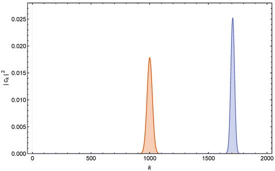
Logically, however, one cannot exclude special cases (e.g., a magnetized piece of metal) with all the spins inside the body oriented in the same direction. One might wonder how the wave function of such a particle with a spin $j\to \infty$ behaves under an inhomogeneous magnetic field. The question is whether the three conditions recognized in [25] required for the emergence of classical mechanics for a macroscopic body with a unique trajectory, reported here in Appendix A, are indeed sufficient. Or is some extra condition, or perhaps a new, unknown mechanism, needed to suppress the possible wide spreading of the wave function into many sub-packets (as is shown in Figure 1 for a small spin, $j=13/2$) under an inhomogeneous magnetic field?

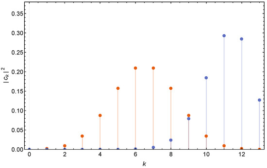
Figure 1. The distribution in $J_z=-j+k$ ($k=0,1,\dots ,2j$) for a spin $j=13/2$ particle in the state in (31) and (32), with $\theta =\pi /2$ (center, orange dots) or with $\theta =\pi /4$ (right, blue dots). The wavepacket of such a particle spreads into many sub-wavepackets à la Stern–Gerlach under an inhomogeneous magnetic field with a strong gradient in the $\widehat{z}$ direction.

This is the central question we are going to investigate. We shall first discuss in Section 2 some mathematical and physical aspects of the quantum states of small and large angular momenta, and compare them with the properties of a classical angular momentum. Considerations of quantum fluctuations of various angular momentum states lead us to propose that a particular class of states, $|j,\mathbf{n}⟩$,

$${\widehat{\mathbf{J}}}^2|j,\mathbf{n}⟩=j(j+1)|j,\mathbf{n}⟩,(\widehat{\mathbf{J}}·\mathbf{n})|j,\mathbf{n}⟩=j|j,\mathbf{n}⟩,$$

(4)

where $\mathbf{n}$ is a unit vector directed towards $(\theta ,\varphi )$ direction,

$$\mathbf{n}=(sin\theta cos\varphi ,sin\theta sin\varphi ,cos\theta ),$$

(5)

or close to them, are to be identified with a classical angular momentum, $j\mathbf{n}$, in the large j limit.

Vice versa, generic states of large spin will be found to remain quantum mechanical, with large fluctuations, even in the limit, $j\to \infty$, showing that the often-stated belief that a large spin (angular momentum) becomes classical should not be taken for granted, literally.

Lest the reader be led to a misunderstanding of the content of our work, let us make the following point clear. The idea that a large spin is made of many spin $\frac{1}{2}$ particles is quite a fruitful one both from mathematical and physical points of view. From the mathematical point of view, the entire theory of angular momentum can indeed be reconstructed this way [27], and it will help to recover certain formulas for large-angular-momentum states easily. It is also useful from physics point of view, as such a system may be regarded as an idealized, toy model for a more realistic macroscopic body, made of many atoms and molecules (carrying spins and orbital angular momenta). And this picture helps interpret some of our findings. (The states of type (4) are known, in the context of many-body systems, as spin coherent states, Bloch states, or Glauber coherent states, depending on the author [5,6,7,9,11,12,15,19,20]. They are all equivalent to the state of definite spin orientation (4), as far as the global spin property is concerned.)

Nevertheless, our discussion is, as will be clear from an attentive reading, entirely about the quantum or classical properties of a single large spin (or angular momentum). We are not concerned here with the thermodynamical or other physical properties of a many-body system. The main question is whether a single large-spin system behaves classically or remains quantum mechanical, in the limit $j/\hslash \to \infty$. As will be seen in the following, the answer turns out to be quite subtle and nontrivial.

In subsequent sections, we are going to examine these questions through the analysis of the Stern–Gerlach processes (Section 3), the orbital angular momenta (Section 4), the angular momentum addition rule (Section 5), and the rotation matrix (Section 6). Generic spin j states far from (4) are shown to remain quantum mechanical even in the limit $j\to \infty$: the fate of these states will be discussed in Section 7. A conclusion and a few more general reflections are given in Section 8.

2. Space of Quantum Spin States and Classical Angular Momenta

The generic pure spin $\frac{1}{2}$ (two-state system) state is described by the vector

$$|\psi ⟩=c_1|\uparrow ⟩+c_2|\downarrow ⟩,$$

(6)

where

$$(c_1,c_2)\sim \lambda (c_1,c_2),\lambda \in \mathbf{C}\backslash \left\{0\right\}$$

(7)

and $|\uparrow ⟩$ and $|\downarrow ⟩$ are spin up and spin down states, i.e., the eigenstates of ${\widehat{J}}_z$ with eigenvalues $\pm \frac{1}{2}$. The complex numbers $(c_1,c_2)$ describe the homogeneous coordinates of the space ${\mathbf{CP}}^1$ ($\sim S^2$). We recall that any state (6) can be interpreted as the state in which the spin is oriented in some direction $\mathbf{n}$,

$$\mathbf{n}=(sin\theta cos\varphi ,sin\theta sin\varphi ,cos\theta ),$$

(8)

that is

$${\widehat{J}}^2\left|{\displaystyle \frac{1}{2}},\mathbf{n}\right.⟩={\displaystyle \frac{3}{4}}\left|{\displaystyle \frac{1}{2}},\mathbf{n}\right.⟩,\left(\widehat{\mathbf{J}}·\mathbf{n}\right)\left|{\displaystyle \frac{1}{2}},\mathbf{n}\right.⟩={\displaystyle \frac{1}{2}}\left|{\displaystyle \frac{1}{2}},\mathbf{n}\right.⟩,$$

(9)

$$|\mathbf{n}⟩\equiv \left|{\displaystyle \frac{1}{2}},\mathbf{n}\right.⟩=c_1|\uparrow ⟩+c_2|\downarrow ⟩,c_1=e^{-i\varphi /2}cos\frac{\theta }{2},c_2=e^{i\varphi /2}sin\frac{\theta }{2}.$$

(10)

without loss of generality. This is so because the space of pure spin $\frac{1}{2}$ quantum states and that of the unit space vector coincide: they are both $S^2\sim {\mathbf{CP}}^1$. Indeed, given State (10), there is always a rotation matrix such that

$$D^{1/2}(0,\theta ,\varphi )·\left(\begin{array}{c}{e}^{-i\varphi /2}cos\frac{\theta }{2}\\ e^{i\varphi /2}sin\frac{\theta }{2}\end{array}\right)=\left(\begin{array}{c}1\\ 0\end{array}\right),$$

(11)

where the general rotation matrix for a spin $\frac{1}{2}$ is given, using Euler angles (note that the third Euler angle (the rotation angle $\gamma$ about the final z-axis) is redundant here, as it gives only the phase $e^{i\gamma /2}$ and has been set to 0 in Equation (11)) ($\gamma ,\theta ,\varphi$), by

$$D^{1/2}(\gamma ,\theta ,\varphi )=U_z\left(\gamma \right)U_y\left(\theta \right)U_z\left(\varphi \right)=\left(\begin{array}{cc}{e}^{i(\gamma +\varphi )/2}cos\frac{\theta }{2}& e^{(\gamma -\varphi )/2}sin\frac{\theta }{2}\\ -e^{i(-\gamma +\varphi )/2}sin\frac{\theta }{2}& e^{-i(\gamma +\varphi )/2}cos\frac{\theta }{2}\end{array}\right).$$

(12)

The fact that any spin $\frac{1}{2}$ quantum state can be associated with a definite space direction, however, does not mean that it can be identified with a classical angular momentum, $\frac{1}{2}\hslash \mathbf{n}$, as the fluctuations in the directions transverse to $\mathbf{n}$ are always of the same order of the spin magnitude itself (see Equation (18) below, with $j=\frac{1}{2}$, $m=\pm \frac{1}{2}$). It is always a quantum mechanical system.

Let us now consider a generic spin j state. It is a special type of $2j+1$-state quantum system. Its general wave function has the form

$$|\psi ⟩=\sum _{m=-j}^j{b}_m|j,j_z=m⟩$$

(13)

where

$$(b_{-j},b_{-j+1},\dots ,b_j)\sim \lambda (b_{-j},b_{-j+1},\dots ,b_j),\lambda \in \mathbf{C}\backslash \left\{0\right\},$$

(14)

are the coordinates of the complex projective space ${\mathbf{CP}}^{2j}$. (As is well known, the manifold of pure quantum states of any n-state system is ${\mathbf{CP}}^{n-1}$ [28]. The spin states (14) are special cases with $n=2j+1$.) On the other hand, the variety of the directions in the three-dimensional space, $\mathbf{n}$, is always $S^2\sim {\mathbf{CP}}^1$. This means that this time not all states of the spin j state given in (13) can be transformed by a rotation matrix (selecting an appropriate new $\widehat{z}$ axis) into the following form:

$$(b_{-j}^{\prime },b_{-j+1}^{\prime },\dots ,b_j^{\prime })\sim (0,0,\dots ,0,1).$$

(15)

This observation is the first hint that there are some subtleties in the way the classical picture of angular momentum emerges from quantum mechanics at large j. It is the purpose of the present paper to elaborate on this point.

Let us start with the basic properties of quantum-mechanical angular momentum. These are of course well-known textbook materials. Because of the commutation relations

$$[{\widehat{J}}_k,{\widehat{J}}_{\mathcal{l}}]=i\hslash {ϵ}^{k\mathcal{l}m}{\widehat{J}}_m,$$

(16)

only one of the components, e.g., ${\widehat{J}}_z$, can be diagonalized together with the total (Casimir) angular momentum, ${\widehat{J}}^2={\widehat{J}}_x^2+{\widehat{J}}_y^2+{\widehat{J}}_z^2$,

$${\widehat{J}}^2|j,m⟩=j(j+1)|j,m⟩,{\widehat{J}}_z|j,m⟩=m|j,m⟩.$$

(17)

In the state $|j,m⟩$, where ${\widehat{J}}_z$ has a definite value, $m\hslash$, ${\widehat{J}}_x$ and ${\widehat{J}}_y$ are fluctuating. Their magnitudes $\Delta J_{x,y}=⟨j,m|{\widehat{J}}_{x,y}^2{|j,m⟩}^{1/2}$ are given by

$$\Delta J_x=\Delta J_y={\left(⟨j,m\left|\left({\widehat{J}}^2-{\widehat{J}}_z^2\right)\right|j,m⟩/2\right)}^{1/2}={\left((j(j+1)-m^2)/2\right)}^{1/2}\hslash \sim \mathcal{O}\left(j\right)\hslash .$$

(18)

Namely, in a generic state $|j,m⟩$, there are strong quantum fluctuations of $J_x$ and $J_y$ at $j\to \infty$, of the same order of magnitude with j itself. There is no way such a state can be associated with a classical angular momentum, which requires all three components to be well-defined simultaneously. The exception occurs for states $|j,\pm j⟩$, for which

$$\Delta {\widehat{J}}_x=\Delta {\widehat{J}}_y={(j/2)}^{1/2}\hslash \ll j\hslash .$$

(19)

For these states, it makes sense to interpret them as a classical angular momentum pointed towards $\pm \widehat{z}$, as its transverse fluctuations $(\sim \mathcal{O}\left(\sqrt{j}\right)$) are negligible with respect to its magnitude j, in the limit $j\to \infty$. The same can be said of the states of spin almost oriented towards $\widehat{z}$, $|j,\pm (j-r)⟩$, $r\ll j$.

Naturally, all states of the form $|j,\mathbf{n}⟩$, in which spin is oriented towards a generic direction $\mathbf{n}$,

$${\widehat{J}}^2|j,\mathbf{n}⟩=j(j+1)|j,\mathbf{n}⟩,\left(\widehat{\mathbf{J}}·\mathbf{n}\right)|j,\mathbf{n}⟩=j|j,\mathbf{n}⟩,$$

(20)

(already defined in (4) in the Introduction) have this property: its fluctuations in the components perpendicular to $\mathbf{n}$ become negligible in the $j\to \infty$ limit. The states given in (20) are known as Bloch states or coherent spin states in the literature [5,6,7,11,12].

These observations lead us to propose that the quantum–classical correspondence (by setting $\hslash =1$) to be made is

$$|j,\mathbf{n}⟩⟷{\mathbf{j}}^{\left(\mathrm{class}\right)}=j\mathbf{n}.$$

(21)

Of course, all states “almost oriented towards $\mathbf{n}$”, $|j,\mathbf{n},q⟩,$

$$\left(\widehat{\mathbf{J}}·\mathbf{n}\right)|j,\mathbf{n},q⟩=(j-q)|j,\mathbf{n},q⟩,q=1,2,\dots ,q\ll j$$

(22)

discussed in Section 3.2.2 (see Equation (53)) below, can also be interpreted as ${\mathbf{j}}^{\left(\mathrm{class}\right)}=j\mathbf{n}$. We are going to examine below the consistency of such a picture, with respect to the SG processes (Section 3 below), a study of orbital angular momentum (Section 4), the addition rule of the angular momenta (Section 5), and the rotation matrix (Section 6).

A powerful idea, useful both for mathematical and physical reasoning below, is that the general spin j can be regarded as a direct product state of $n=2j$ spins, each carrying $\frac{\hslash }{2}$. From a group-theoretic point of view, it is well known that any irreducible representation of the SU(2) group, which is the double covering group (see e.g., [29]) of the rotation group SO(3), is associated with the Young tableaux

$$\underset{n\mathrm{boxes}}{\underbrace{☐☐☐\dots ☐}},$$

(23)

with a single row of n boxes, i.e., the totally symmetric direct product of $n=2j$ spin $\frac{1}{2}$ objects. Indeed, the entire theory of quantum angular momentum can be reconstructed based on this point of view [27] by using the operators

$${\widehat{J}}^a=\sum _{i,j=1,2}{a}_i^{†}{\left({\displaystyle \frac{{\tau }^a}{2}}\right)}_{ij}{a}_j,[{\widehat{J}}^a,{\widehat{J}}^b]=i{ϵ}_{abc}{\widehat{J}}^c,$$

(24)

where ${\tau }^a$ are the Pauli matrices, and $a_i$ and $a_i^{†}$ are the harmonic-oscillator annihilation and creation operators of spin-up ($i=1$) and spin-down ($i=2$) particles, given by

$$[a_i,a_j^{†}]={\delta }_{ij}.$$

(25)

By construction, all states $\propto a_1^{†}{a}_2^{†}{a}_1^{†}{a}_1^{†}\dots |0⟩$, with k$a_1^{†}$’s and $(N-k)$$a_2^{†}$’s ($k=0,1,2,\dots N$), are symmetric under exchanges of the spins, and therefore belong to the irreducible representation $\underline{j}$, with $j=N/2$. (An analogous construction for the $SU\left(N\right)$ group, $N\ge 3$, is possible, but only for totally symmetric representations, $☐☐☐\dots ☐$. The usefulness of such an approach is somewhat limited compared to the $SU\left(2\right)$ case, where any irreducible representation has this form. But the construction analogous to (24) for $SU\left(N\right)$ can explain, for instance, the degeneracy of the energy eigenstates of the N-dimensional isotropic harmonic oscillator.)

Physically, on the other hand, one may consider (23) a particular state of a toy-model macroscopic body made of n atoms, each carrying spin $\frac{1}{2}$.

Now a particularly attractive picture of the quantum states in (23) of general spin j follows from the so-called stellar representation of ${\mathbf{CP}}^n$ ($n=2j$) [28]. Let the complex numbers

$$(Z_0,Z_1,\dots ,Z_n)\sim \lambda (Z_0,Z_1,\dots ,Z_n),\lambda \in \mathbf{C}\backslash \left\{0\right\}$$

(26)

be the homogeneous coordinates of ${\mathbf{CP}}^n$, and consider the n-th order equation

$$\sum _{k=0}^n{Z}_k{z}^{n-k}=Z_0\prod _{\mathcal{l}=1}^n(z-w_{\mathcal{l}})=0.$$

(27)

As Equation (27) is invariant under the rescaling given in (26), the collection of the n roots for z, $\left\{w_{\mathcal{l}}\right\}$, can each be regarded as equivalent to a point of ${\mathbf{CP}}^n$. Note that no generality is lost by considering the neighborhood $Z_0\ne 0$ above: for instance, one may introduce the variable $z^{\prime }\equiv 1/z$ and rewrite Equation (27) in terms of $z^{\prime }$. One sees then that the equation with $Z_0=0$ contains (at least one) root $z^{\prime }=0$, that is, $z=\infty$.

The explicit relation between $\left\{w_{\mathcal{l}}\right\}$ and the ${\mathbf{CP}}^n$ point can be found by working backward: given any collection of n roots $\left\{w_{\mathcal{l}}\right\}$ in the complex plane, one can find the coefficients $\left\{Z_k\right\}$—the coordinates of ${\mathbf{CP}}^n$—by simply expanding the second expression of (27). The connection between this construction and the picture (23) above comes from the fact that any complex number $\left\{w_{\mathcal{l}}\right\}$ can be regarded as the stereographic projection of a point on a sphere $S^2$, from the north (or south) pole, onto the plane containing the equator. See Figure 2. Naturally, a point on $S^2$ can be identified with the unit vector $\mathbf{n}$, (8), the orientation of each component spin $\frac{1}{2}$. The explicit relation is

$$w_{\mathbf{n}}={\displaystyle \frac{e^{i\varphi }}{tan(\theta /2)}}.$$

(28)

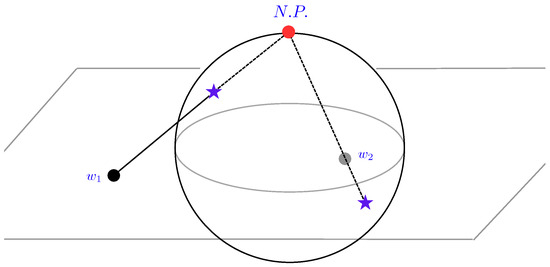
Figure 2. Two points (stars) on the sphere and their stereographic projections from the north pole (N.P.) onto the plane containing the equator.

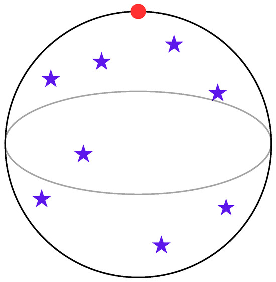
Summing up, we see that a point in ${\mathbf{CP}}^n$ is represented by an unordered collection of n points on a sphere (stars); see Figure 3. This is known as the stellar representation of ${\mathbf{CP}}^n$.

Figure 3. A general point in ${\mathbf{CP}}^n$ is equivalent to an unordered collection of n points (stars) on a sphere, in the stellar representation (27). Each star is associated with the complex number $w_{\mathcal{l}}$ by a stereographic projection, as in Figure 2.

From the group-theoretic point of view, (23), a generic quantum state of spin j, is equivalent to the collection (the direct product) of $n=2j$ spin $\frac{1}{2}s$

$$\mathcal{S}|{\mathbf{n}}_1⟩|{\mathbf{n}}_2⟩\dots |{\mathbf{n}}_n⟩$$

(29)

where $\mathcal{S}$ stands for a symmetrization, orientated towards various directions ${\mathbf{n}}_k$, $k=1,2,\dots ,n$; see Equation (10). The state given in (29) represents a general state of spin $j=2n$ and naturally corresponds to the random sets of stars in Figure 3.

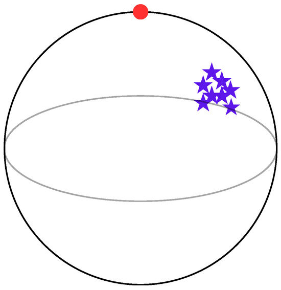
The particular state in which the spin j is oriented towards a definite direction $\mathbf{n}$, (20), corresponds to the case in which the component $\frac{1}{2}$ spins are all oriented towards the same direction ${\mathbf{n}}_1={\mathbf{n}}_2=\dots ={\mathbf{n}}_n=\mathbf{n}$,

$$|j,\mathbf{n}⟩=|\mathbf{n}⟩|\mathbf{n}⟩\dots |\mathbf{n}⟩$$

(30)

(which is automatically symmetric). See Figure 4. By using (10) for each $|\mathbf{n}⟩$ and collecting terms with the same fixed number k of the spin-up factors, we find $|j,\mathbf{n}⟩$ as an expansion in terms of the eigenstates of $J_z$ with $J_z=m$,

$$|j,\mathbf{n}⟩=\sum _{k=0}^{2j}{c}_k|j,m⟩,m=-j+k,$$

(31)

$$c_k={\left({\displaystyle \genfrac{}{}{0pt}{}{2j}{k}}\right)}^{1/2}{e}^{i(j-k)\varphi }{\left(cos\frac{\theta }{2}\right)}^k{\left(sin\frac{\theta }{2}\right)}^{2j-k},\sum _{k=0}^{2j}{\left|c_k\right|}^2=1,$$

(32)

where $\left(\genfrac{}{}{0pt}{}{n}{k}\right)=n!/k!(n-k)!$ are the binomial coefficients. States (31) and (32) coincide, apart from an overall phase factor, with the Bloch (or spin coherent) states considered in the many-body physics context [5,6,7,9,11,12,15,19,20], denoted as $|j,\mathrm{\Omega }⟩$, $|j,\{\theta ,\varphi \}⟩$, etc.

Figure 4. The coherent spin state given in (20), (31), and (32) in the stellar representation.

In order to understand this formula from the point of view of the stellar representation of ${\mathbf{CP}}^n$, we need to translate the homogeneous coordinates of ${\mathbf{CP}}^n$ to the coefficients $\left\{c_k\right\}$ in (31) as

$$Z_k=c_k^2,k=0,1,\dots ,n,$$

(33)

and at the same time replace the projection of the stars on $S^2$ as

$$w_{\mathcal{l}}\to w_{\mathcal{l}}^2,\forall \mathcal{l}.$$

(34)

Equations (33) and (34) reflect the double covering of the SO(3) group by SU(2).

In the stellar representation of ${\mathbf{CP}}^n$, given by (26) and (27), State (30) corresponds to the situation where all roots coincide,

$$w_{\mathcal{l}}=w_{\mathbf{n}},\forall \mathcal{l}.$$

(35)

All stars are at a coincident point $\mathbf{n}$ on the sphere; see Figure 4.

Taking into account the doubling in (33) and (34) and expanding ($n=2j$)

$$\sum _{k=0}^n{\left(c_k\right)}^2{z}^{n-k}=\prod _{\mathcal{l}=1}^n(z-w_{\mathcal{l}}^2)={(z-w_{\mathbf{n}}^2)}^n,$$

(36)

($w_{\mathbf{n}}={\displaystyle \frac{e^{i\varphi }}{tan(\theta /2)}}$), one finds precisely (31) and (32), apart from unobservable phases and an overall factor.

Thus the stellar representation of ${\mathbf{CP}}^n$ points—the generic states of spin j—provides us with an appealing intuitive picture of quantum fluctuations. The ${\mathbf{CP}}^n$ points with randomly distributed stars, as given in Figure 3, represent spin states with large quantum fluctuations. The special states, (20) and (30)–(32) with coincident stars (see Figure 4), are those with minimum fluctuations, and they correspond to the Bloch or spin coherent state [5,6,7,11,12]. In the next four sections, we shall illustrate how these states effectively behave as classical angular momenta, $j\mathbf{n}$, in the $j\to \infty$ limit.

3. Stern–Gerlach Experiments

In this section we compare the Stern–Gerlach experiment [30] for small and large spins, with special attention to the states, (20), (31), and (32).

3.1. Spin 1/2 Atom

For definiteness let us take an incident atom with spin $j=\frac{1}{2}$ directed along a definite, but generic, direction $\mathbf{n}=(sin\theta cos\varphi ,sin\theta sin\varphi ,cos\theta )$—i.e.,

$$\mathsf{\Psi }=\psi (\mathbf{r},t)|\mathbf{n}⟩,$$

(37)

$$|\mathbf{n}⟩=c_1|\uparrow ⟩+c_2|\downarrow ⟩,c_1=e^{-i\varphi /2}cos\frac{\theta }{2},c_2=e^{i\varphi /2}sin\frac{\theta }{2}.$$

(38)

Let us suppose that the atom enters from $x=-\infty$ and moves towards $x=+\infty$. When the atom passes through a region with an inhomogeneous magnetic field with

$${\displaystyle \frac{\partial B_z}{\partial z}}\ne 0,$$

(39)

the wave packet splits into two subpackets, with respective weights $|c_1{|}^2$ and $|c_2{|}^2$: they manifest as the relative intensities of the two separate image bands on the screen at the end.

Even though the Stern–Gerlach process is discussed in every textbook on quantum mechanics, there is a subtlety that is relatively little known. The (apparent) puzzle is why the net effect is the deflection of the atom towards the $\pm \widehat{z}$ direction only, in spite of the fact that Maxwell’s equations, $\nabla ·\mathbf{B}=0$ and $\nabla \times \mathbf{B}=0$, dictate that the inhomogenuity (39) implies an inhomogenuity $\partial B_y/\partial y$ of the same magnitude (assuming $B_x=0$). The explanation, with a discussion on the characteristics of the appropriate magnetic fields, has been given in [31,32]. We briefly review this story in Appendix B.

The original Stern–Gerlach experiment (1922) [30] has had a fundamental impact on the development of quantum theory, proving the quantization of angular momentum, proving the existence of half-integer spin, and more generally, demonstrating the quantum-mechanical nature of the silver atom as a whole [26].

The wave function of the form (38) corresponds to a pure state, i.e., 100% polarized beam, where all incident atoms are in the same spin state. If the beam is partially polarized or unpolarized, the state is described by a generic density matrix $\rho$, with

$$Tr\rho =1,{\rho }_{ii}\ge 0,i=1,2.$$

(40)

The Stern–Gerlach experiment measures the relative frequency that the atom arriving at the screen happens to have, whether spin $s_z=\frac{1}{2}$ or spin $s_z=-\frac{1}{2}$. Let

$${\mathrm{\Pi }}_{\uparrow }=|\uparrow ⟩⟨\uparrow |=\left(\begin{array}{cc}1& 0\\ 0& 0\end{array}\right),{\mathrm{\Pi }}_{\downarrow }=|\downarrow ⟩⟨\downarrow |=\left(\begin{array}{cc}0& 0\\ 0& 1\end{array}\right)$$

(41)

be the projection operators on the spin up (down) states; the relative intensities of the upper and lower blots on the screen are, according to QM,

$${\overline{\mathrm{\Pi }}}_{\uparrow }=Tr{\mathrm{\Pi }}_{\uparrow }\rho ={\rho }_{11};{\overline{\mathrm{\Pi }}}_{\downarrow }=Tr{\mathrm{\Pi }}_{\downarrow }\rho ={\rho }_{22},{\rho }_{11}+{\rho }_{22}=1.$$

(42)

The prediction concerning the relative intensities of the two narrow atomic image bands from the wave function (38) and from the density matrix (42) is in general indistinguishable, as is well known.

3.2. Large Spin

Consider now the state of a spin j directed towards a direction $\mathbf{n}$, $|j,\mathbf{n}⟩$, as given in (20), (31), and (32); see Figure 4. Choosing the magnetic field (and its gradients) in the z-direction, we need to express $|j,\mathbf{n}⟩$ as a superposition of the eigenstates of ${\widehat{J}}_z$ ($j=n/2$). This is precisely the expression given in Equations (31) and (32).

Using Stirling’s formula in (32), one finds, for n and $k=j+m$ both large with $x=k/n$ fixed, the following distribution in different values of $m=-j+k$:

$$|c_k{|}^2\simeq e^{nf\left(x\right)},x=k/n=(j+m)/2j,$$

(43)

where

$$f\left(x\right)=-xlogx-(1-x)log(1-x)+2xlogcos\frac{\theta }{2}+2(1-x)logsin\frac{\theta }{2}.$$

(44)

The saddle-point approximation valid at $n\to \infty$ yields

$$f\left(x\right)\simeq -{\displaystyle \frac{{(x-x_0)}^2}{x_0(1-x_0)}},x_0={cos}^2\frac{\theta }{2},$$

(45)

and therefore

$$\sum _k{\left|c_k\right|}^2(\dots )⟶{\int }_0^{1}dx\delta (x-x_0)(\dots )$$

(46)

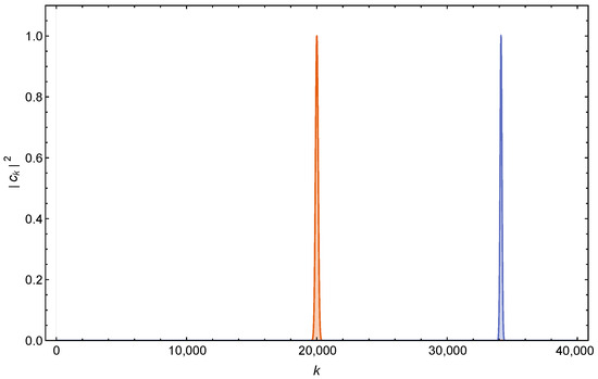
in the $n\to \infty$ ($x=k/n$ fixed) limit. The narrow peak position $x=x_0$ corresponds to (see Equation (31))

$$J_z=m=n(x-\frac{1}{2})=j(2{cos}^2\frac{\theta }{2}-1)=jcos\theta .$$

(47)

This means that a large spin ($j\gg \hslash$) quantum particle with spin directed towards $\mathbf{n}$, in a Stern–Gerlach setting with an inhomogeneous magnetic field (39), moves along a single trajectory of a classical particle with $J_z=jcos\theta$, instead of spreading over a wide range of split sub-packet trajectories covering $-j\le m\le j$. See Figure 5 (spin $j={10}^3$) and Figure 6 ($j=2·{10}^5$) and compare them with Figure 1 for spin $j=13/2$.

Figure 5. A distribution in possible values of $J_z=-j+k$, for a spin $j=1·{10}^3$ particle in States (31) and (32), with $\theta =\pi /2$ (center, orange peak) or with $\theta =\pi /4$ (right, blue peak). The graph represents the distribution $|c_k{|}^2$. The particle starts looking like classical.

Figure 6. The distribution in $J_z$ ($\equiv -j+k$) as in Figure 5 but for a spin $j=2·{10}^5$, for $\theta =\pi /2$ (center, orange peak) or $\theta =\pi /4$ (right, blue peak). This figure was drawn by using the approximations (43) and (44), rather than the exact formula, given by (31) and (32).

This (perhaps) somewhat surprising result appears to indicate that quantum mechanics (QM) takes care of itself, so to speak, in ensuring that a large-spin particle ($j/\hslash \to \infty$) behaves classically, at least for these particular states $|j,\mathbf{n}⟩$. No extra conditions are necessary. This is consistent with the known general behavior of the wave function in the semi-classical limit ($\hslash \to 0$) (Of course this does not mean that the classical limit necessarily requires or implies $j/\hslash \to \infty$). Note that if the value $j\gg \hslash$ is understood as due to the large number of spin ${\displaystyle \frac{1}{2}}$ particles composing it (see the comment after (32)), the spikes given by (45) and (46) can be understood as due to the accumulation of a huge number of microstates giving $J_z\simeq m$.

Another, equivalent way to see the shrinkage of the distribution in $J_z=m$, (46), is to study its dispersion. Given the relative weights $|c_k{|}^2$, (32), where $m=-j+k$ and $j=\frac{n}{2}$, with $k=0,1,\dots ,n$, it is a simple exercise to find that

$$⟨J_z⟩=jcos\theta ,⟨J_z^2⟩=j^2{cos}^2\theta +{\displaystyle \frac{j}{2}}{sin}^2\theta ,$$

(48)

so that the dispersion (the fluctuation width) is given by (these results are well known [11])

$${(\Delta J_z)}^2=⟨{(J_z-⟨J_z⟩)}^2⟩=⟨J_z^2⟩-{⟨J_z⟩}^2={\displaystyle \frac{j}{2}}{sin}^2\theta .$$

(49)

It follows that

$$\underset{j/\hslash \to \infty }{lim}{\displaystyle \frac{|\Delta J_z|}{j}}=0,$$

(50)

i.e., it is an infinitely narrow distribution. Note that the SG experiment is indeed a measurement of $J_z$ in State (31). The fact that the result is always $J_z\sim ⟨J_z⟩=jcos\theta$ with no dispersion means that it is a classical angular momentum $\sim j\mathbf{n}$.

3.2.1. State Preparation and Successive SG Set-Ups

For a small j, as is well known, the SG set-up can be used to prepare any desired state $|j,J_z=m⟩$ using an intentionally biased SG apparatus, e.g., in which all the split sub-wavepackets are blocked, except for the one corresponding to $|j,m⟩$. Equivalently, one may use the so-called null-measurements (see Ref. [33] for a recent review). In any case, for a small finite j, where there are $2j+1$ well-separated sub-packets (see Figure 1), there is no difficulty in extracting any desired quantum state for subsequent experiments (state preparation).

In the large-spin limit ($j\to \infty$) of the Bloch states $|j,\mathbf{n}⟩$ we are considering, there is no possibility of extracting or selecting a desired sub-wavepacket, since there is essentially only one narrow wavepacket present (see (47) and Figure 6). Trying to extract a state with $J_z$ not close to $jcos\theta$ would simply give a zero result. We have in mind a macroscopic scenario where, in comparison to the finite region (in principle) occupied by the waves $-j\le m\le j$, the fluctuations of the values of m around (47) are of the order $\sqrt{j}\ll j$, i.e., of zero width.

We might consider introducing a second set of Stern–Gerlach (SG) magnetic fields directed in a different direction, denoted by ${\widehat{z}}^{\prime }$, as a new quantization axis. This set-up allows us to study the state emerging from the first set of SG magnetic fields (but without an imaging screen),

$$|j,\mathbf{n}⟩\sim c_k|j,J_z=m⟩,m\sim jcos\theta .$$

(51)

Since the sum of states around $m\sim jcos\theta$ is essentially equal to the complete sum, this state can be rewritten as

$$\begin{array}{ccc}\hfill |j,\mathbf{n}⟩& =& \sum _{m,m^{\prime }}{c}_k|j,m^{\prime }⟩⟨j,m^{\prime }|j,m⟩\hfill \\ & =& \sum _{m,m^{\prime }}|j,m^{\prime }⟩⟨j,m^{\prime }|j,m⟩⟨j,m|j,\mathbf{n}⟩\hfill \\ & =& \sum _{m^{\prime }}|j,m^{\prime }⟩⟨j,m^{\prime }|j,\mathbf{n}⟩=\sum _{m^{\prime }}{c}_{k^{\prime }}|j,m^{\prime }⟩,\hfill \end{array}$$

(52)

where in the first line a completeness relation ${\sum }_{m^{\prime }}|j,m^{\prime }⟩⟨j,m^{\prime }|=\mathbf{1}$ has been inserted, and in the second we recall $c_k=⟨j,m|j,\mathbf{n}⟩$ (see Equation (31)). Equation (52) represents an expansion of the original state $|j,\mathbf{n}⟩$ as a linear combination of the eigenstates of $J_{z^{\prime }}=m^{\prime }$. In the limit $j\to \infty$, the results from Section 3.2 tell us that the sum is dominated by the small region around $m^{\prime }\sim jcos(\mathbf{n}·{\widehat{z}}^{\prime })$, with negligible fluctuations. The trajectory remains unique, regardless of the choice of quantization axis (i.e., the direction of the magnetic field) ${\widehat{z}}^{\prime }$.

3.2.2. States Almost Directed Towards $\overrightarrow{\mathbf{n}}$

Obviously, in the large-spin limit, other states close to $|j,\mathbf{n}⟩$,

$$\left(\widehat{\mathbf{j}}·\mathbf{n}\right)|j,\mathbf{n},q⟩=(j-q)|j,\mathbf{n},q⟩,q=1,2,\dots \mathrm{fixed}$$

(53)

(i.e., the spin roughly oriented towards $\mathbf{n}$) will behave similarly. For instance, the $q=1$ state is (cfr. Equation (31))

$$\begin{array}{ccc}\hfill |j,\mathbf{n},1⟩& =& \sum _{\mathcal{l}=0}^{N-1}{\displaystyle \frac{1}{\sqrt{N}}}{|\mathbf{n}⟩}_1\otimes {\dots |\mathbf{n}⟩}_{\mathcal{l}}{\otimes |-\mathbf{n}⟩\otimes |\mathbf{n}⟩}_{\mathcal{l}+2}\otimes \dots {|\mathbf{n}⟩}_N,\hfill \\ & =& \sum _{\mathcal{l}=0}^{N-1}{\displaystyle \frac{1}{\sqrt{N}}}|j_1,\mathbf{n}⟩\otimes |-\mathbf{n}⟩\otimes |j_2,\mathbf{n}⟩,\hfill \end{array}$$

(54)

where $|j_1,\mathbf{n}⟩$ and $|j_2,\mathbf{n}⟩$ ($j_1=\frac{\mathcal{l}}{2},j_2=\frac{N-\mathcal{l}-1}{2}$), are two spins oriented towards $\mathbf{n}$ (20), as already studied in Section 3.2. In the $j\to \infty$ limit, the sum is dominated by terms with $\mathcal{l}\sim \mathcal{O}\left(N\right)\to \infty$. The SG projection of this state onto the $j_z$ eigenstates is therefore approximated by

$$j_z\sim j_{1z}+j_{2z}=j_{1}cos\theta +j_{2}cos\theta \simeq jcos\theta ,$$

(55)

where the results of Section 3.2 have been used. A similar result holds for $|j,\mathbf{n},q⟩$ for any finite q, showing that all these states behave as a classical angular momentum, $j\mathbf{n}$.

4. Orbital Angular Momentum

All our formal arguments (16)–(22) apply equally well both to spin (the intrinsic angular momentum of a particle or the total angular momentum of the center of mass of a body in its rest frame) and to orbital angular momentum. However, our primary tool of analysis is the Stern–Gerlach (SG) set-up (Section 3.2), which is more suitable for spin than for an angular momentum associated with the orbital motion of a particle. One might wonder how the large-angular-momentum limit works for the latter. Here is a brief account.

The (angular part of the) wave function of a particle in the state $|\mathcal{l},m⟩$ corresponds to the spherical harmonics

$$⟨\theta ,\varphi |\mathcal{l},m⟩=Y_{\mathcal{l},m}(\theta ,\varphi )={(-)}^{(m+|m\left|\right)}\sqrt{\frac{(2\mathcal{l}+1)(\mathcal{l}-|m\left|\right)!}{4\pi (\mathcal{l}+|m\left|\right)!}}{P}_{\mathcal{l}}^{\left|m\right|}\left(x\right)e^{im\varphi },x\equiv cos\theta ,$$

(56)

where $P_{\mathcal{l}}^m\left(x\right)$ gives the associated Legendre polynomials. Let us consider the state of minimum fluctuation, $|\mathcal{l},\mathcal{l}⟩$ (see Equation (19)). It is easy to see that the angular distribution is strongly peaked at $\theta =\frac{\pi }{2}$ at large $\mathcal{l}$:

$$|Y_{\mathcal{l},\mathcal{l}}{(\theta ,\varphi )|}^2={\displaystyle \frac{2\mathcal{l}+1}{4\pi }}{\displaystyle \frac{\left(2\mathcal{l}\right)!}{2^{2\mathcal{l}}{(l!)}^2}}{(1-x^2)}^{\mathcal{l}}\stackrel{\mathcal{l}\to \infty }{⟶}{\displaystyle \frac{1}{2\pi }}\delta \left(x\right).$$

(57)

For instance, see Figure 7 for $\mathcal{l}=m={10}^3$. In states $|\mathcal{l},m⟩$ with stronger fluctuations, with m not close to $\pm \mathcal{l}$, the distribution instead covers a large portion of the 3D solid angle, for any $\mathcal{l}$ (see Figure 8 for $\mathcal{l}=100,m=50$).

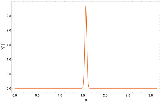
Figure 7. The distribution in $\theta$, for the state $|\mathcal{l},\mathcal{l}⟩$ with $\mathcal{l}={10}^3$.

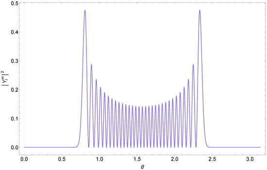
Figure 8. The distribution in $\theta$, for the state $|\mathcal{l},m⟩$ with $\mathcal{l}=100$, $m=50$.

Now a classical angular momentum has its all three components well defined. By choosing an appropriate coordinate system, it can be written as ${\mathbf{L}}^{\left(\mathrm{class}\right)}=(0,0,L)$. It describes a particle moving in the $(x,y)$ plane, with $z=p_z=0$. The large $\mathcal{l}$ limit of the wave function $|Y_{\mathcal{l},\mathcal{l}}{(\theta ,\varphi )|}^2$, (57), describes precisely such a motion.

5. Addition of Angular Momenta

Let us now consider two spins, ${\mathbf{j}}_1$ and ${\mathbf{j}}_2$. The composition–decomposition rule in QM is well known—i.e.,

$$\underline{j_1}\otimes \underline{j_2}=\underline{j_1+j_2}\oplus \underline{j_1+j_2-1}\oplus \dots \underline{|j_1-j_2|},$$

(58)

where $\underline{j}$ indicates the multiplet (the irreducible representation) of SU(2) (we recall that SU(2) is the simply connected double cover of the orthogonal group SO(3)), with multiplicity $2j+1$ and with $max\left\{j_z\right\}=j$. We set $\hslash =1$ here.

We wish to find out how the addition rule looks in the limit $j_1,j_2\to \infty$. We are particularly interested in the composition rule for angular momentum states with minimum fluctuations of the form $|j,\mathbf{n}⟩$. Therefore, let us consider two particles (spins) in the states

$${\widehat{\mathbf{j}}}_1·{\mathbf{n}}_1|j_1,{\mathbf{n}}_1⟩=j_1|j_1,{\mathbf{n}}_1⟩,{\widehat{\mathbf{j}}}_2·{\mathbf{n}}_2|j_2,{\mathbf{n}}_2⟩=j_2|j_2,{\mathbf{n}}_2⟩,$$

(59)

namely, they are spins oriented towards the directions ${\mathbf{n}}_1$ and ${\mathbf{n}}_2$, respectively. Our aim is to find out the properties of the direct product state

$$|j_1,{\mathbf{n}}_1⟩\otimes |j_2,{\mathbf{n}}_2⟩,$$

(60)

in the large $j_1,j_2$ limit.

Since the choice of the axes is arbitrary; we may take

$${\mathbf{n}}_2=(0,0,1).$$

(61)

Then the product state is just

$$|j_1,{\tilde{\mathbf{n}}}_1⟩\otimes |j_2,m_2=j_2⟩,$$

(62)

where $|j_2,m_2=j_2⟩$ is the highest ${\widehat{j}}_{2z}$ state. We added the tilde sign on ${\mathbf{n}}_1$ to indicate that it is the vector ${\mathbf{n}}_1$ in the reference system, (61). Now $|j_1,{\tilde{\mathbf{n}}}_1⟩$ in the $j_1\to \infty$ limit has been studied in Section 3.2. It is

$$|j_1,{\tilde{\mathbf{n}}}_1⟩=\sum _{m=-j_1}^{j_1}{c}_m|j_1,j_{1z}=m⟩,$$

(63)

where the sum is dominated by the values of m around

$$m=j_{1z}=j_{1}cos\theta ,cos\theta ={\tilde{\mathbf{n}}}_{1z}={\mathbf{n}}_1·{\mathbf{n}}_2,$$

(64)

with the fluctuations of $j_{1z}$, which become negligible in the infinite spin limit (see Figure 6). For the purpose of the discussion of this section, we introduce the notation

$$|j_1,{\tilde{\mathbf{n}}}_1⟩\simeq |j_1,j_{1z}=j_{1}cos\theta ⟩,$$

(65)

by using the ≃ sign, to express this fact. Since the eigenvalues of ${\widehat{j}}_z$ simply add up in the product state, the expansion of $|j_1,{\mathbf{n}}_1⟩\otimes |j_2,{\mathbf{n}}_2⟩$ in the expansion in terms of the eigenstates of ${\widehat{j}}_{\mathrm{tot}z}$ is dominated by terms with $j_{\mathrm{tot}}^{{\tilde{n}}_2}=j_{1}cos\theta +j_2$, namely,

$$|j_1,{\mathbf{n}}_1⟩\otimes |j_2,{\mathbf{n}}_2⟩\simeq |j_{\mathrm{tot}},j_{\mathrm{tot}}^{{\tilde{n}}_2}=j_{1}cos\theta +j_2⟩,$$

(66)

where $j_{\mathrm{tot}}^{{\tilde{n}}_2}$ means the component in the direction of ${\tilde{n}}_2$ of the (for the moment, unknown) total spin $j_{\mathrm{tot}}$. Exchanging ${\mathbf{n}}_1$ and ${\mathbf{n}}_2$ and repeating the arguments, one finds also that

$$|j_1,{\mathbf{n}}_1⟩\otimes |j_2,{\mathbf{n}}_2⟩\simeq |j_{\mathrm{tot}},j_{\mathrm{tot}}^{{\tilde{n}}_1}=j_1+j_{2}cos\theta ⟩.$$

(67)

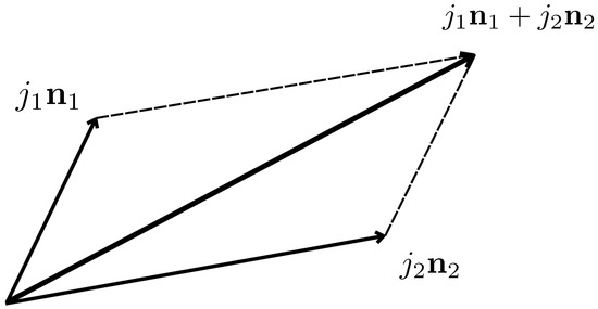
But which quantum angular-momentum state does the product state given in (60) represent? Such a state must be compatible with the projections given in (66) and (67). The answer is that

$$|j_1,{\mathbf{n}}_1⟩\otimes |j_2,{\mathbf{n}}_2⟩\simeq |j_{\mathrm{tot}},\mathbf{n}⟩,$$

(68)

with $j_{\mathrm{tot}}$ and the unit vector $\mathbf{n}$ defined by

$$j_{\mathrm{tot}}\mathbf{n}=j_1{\mathbf{n}}_1+j_2{\mathbf{n}}_2.$$

(69)

Note that this (classical) vector sum determines both $j_{\mathrm{tot}}$ (the magnitude) and $\mathbf{n}$ (the direction) uniquely. The quantum state $|j_{\mathrm{tot}},\mathbf{n}⟩$ is defined via the correspondences in (20) and (21) proposed before.

The proof of Statement (68) is as follows. By selecting the directions of the SG magnet directions (the quantization axis) to ${\mathbf{n}}_2$ or to ${\mathbf{n}}_1$ on the state $|j_{\mathrm{tot}},\mathbf{n}⟩$, (69), one can apply the results of Section 3.1 to obtain exactly the results of (66) or (67), respectively. Now, according to the quantum–classical correspondence of Equation (21), the state $|j_{\mathrm{tot}},\mathbf{n}⟩$ (see Equation (69)) translates into

$${\mathbf{j}}_{\mathrm{tot}}^{\left(\mathrm{class}\right)}=j_1{\mathbf{n}}_1+j_2{\mathbf{n}}_2.$$

(70)

But, in view of (21), this is precisely the addition rule of the two classical angular momenta.

To be complete, one must check that the projection on any other generic direction ${\mathbf{n}}_3$ works correctly. By using the result of Section 3.2 for the SG projection on a new ${\mathbf{n}}_3$ axis, one finds

$$|j_1,{\mathbf{n}}_1⟩\otimes |j_2,{\mathbf{n}}_2⟩\simeq |j_{\mathrm{tot}}^{\prime },j_{\mathrm{tot}}^{\prime n_3}=j_1{\mathbf{n}}_1·{\mathbf{n}}_3+j_2{\mathbf{n}}_2·{\mathbf{n}}_3⟩,$$

(71)

where we make use of the fact that ${\widehat{\mathbf{j}}}_1$ and ${\widehat{\mathbf{j}}}_2$ commute and the eigenvalues of their ${\mathbf{n}}_3$ components simply sum up in the direct product state. Also, to be conservative, we have left $j_{\mathrm{tot}}^{\prime }$ unknown. But

$$j_1{\mathbf{n}}_1·{\mathbf{n}}_3+j_2{\mathbf{n}}_2·{\mathbf{n}}_3=(j_1{\mathbf{n}}_1+j_2{\mathbf{n}}_2)·{\mathbf{n}}_3,$$

(72)

and therefore

$${\mathbf{j}}_{\mathrm{tot}}^{\prime }={\mathbf{j}}_{\mathrm{tot}}=j_1{\mathbf{n}}_1+j_2{\mathbf{n}}_2,$$

(73)

by again using the results of Section 3.1 in Equation (71), which proves Equations (68) and (69). In conclusion, the direct product state, given in (59) and (60), has a simple classical interpretation. It corresponds to the classical sum (the vector addition) of two angular momenta; see Figure 9.

Figure 9. The direct product state, (60), behaves as a classical vector sum in the limit, $j_1,j_2\to \infty$, in the sense of the correspondence in (21).

From the perspective of the general composition rule of two angular momentum states (58), what we have seen are the results concerning a specific pair of states (i.e., those of minimum fluctuations) in $\underline{j_1}$ and $\underline{j_2}$, characterized by the “orientations” ${\mathbf{n}}_1$ and ${\mathbf{n}}_2$. The total angular momentum magnitude in the product state given in (68) and (69) satisfies

$$j_1+j_2\ge j_{\mathrm{tot}}=|j_1{\mathbf{n}}_1+j_2{\mathbf{n}}_2|\ge |j_1-j_2|,$$

(74)

depending on the relative orientation of ${\mathbf{n}}_1$ and ${\mathbf{n}}_2$. Equation (74) is nicely consistent with the quantum-mechanical composition law given in (58).

Spin–Orbit Interactions

As a possible variation of theme, and for completeness, let us consider a spin–orbit interaction of the form

$$H=A\mathbf{L}·\mathbf{S}$$

(75)

where A is a constant, and $\mathbf{L}$ and $\mathbf{S}$ are the orbital angular momentum and spin, respectively, of a given system. The problem is to understand whether and/or how such an interaction Hamiltonian reduces effectively to an interaction between two classical angular momenta in the limits $L/\hslash \to \infty$ and $S/\hslash \to \infty$. By writing

$$H={\displaystyle \frac{A}{2}}({\mathbf{J}}^2-{\mathbf{L}}^2-{\mathbf{S}}^2),\mathbf{J}=\mathbf{L}+\mathbf{S},$$

(76)

and assuming that ${\mathbf{L}}^2$ and ${\mathbf{S}}^2$ have fixed values $L(L+1){\hslash }^2$ and $S(S+1){\hslash }^2$ in the system under consideration, the problem reduces to that of angular momentum addition, already considered in this section. As such, an interaction of the form (75) would reduce to its classical counterpart, when the two states with angular momentum moduli L and S are the states of minimum fluctuations, such as $|\mathcal{l},\mathcal{l}⟩$ of (57) and $|j,\mathbf{n}⟩$ of (20).

On the other hand, for generic atomic states such conditions are not expected to be satisfied, even in the limit of large atoms. Thus the discussion of this section is mostly irrelevant, and the standard, quantum mechanical analysis of spin–orbit interactions is always required.

6. Rotation Matrix

The rotation matrix for a general spin j can be constructed by taking the direct products of the rotation matrix for spin $\frac{1}{2}$, i.e., (12). This is based on the fact that any angular momentum state, $|j,m⟩$, can be constructed as a system made of N spin $\frac{1}{2}$ particles, completely symmetric under exchange of the particles, a fact already conveniently used in Section 3.1. The rotation matrix for a generic spin j is simply (writing the Euler angles symbolically as $\mathrm{\Omega }\equiv \{\gamma ,\theta ,\varphi \}$) the direct productof the rotation matrices for spin $\frac{1}{2}$, (12),

$${\left(D^j\left(\mathrm{\Omega }\right)\right)}_{M,M^{\prime }}=\mathcal{S}\left[{\left(D^{1/2}\left(\mathrm{\Omega }\right)\right)}_{m_1,m_1^{\prime }}{\left(D^{1/2}\left(\mathrm{\Omega }\right)\right)}_{m_2,m_2^{\prime }}\dots {\left(D^{1/2}\left(\mathrm{\Omega }\right)\right)}_{m_N,m_N^{\prime }}\right]$$

(77)

symmetrized ($\mathcal{S}$) with respect to $(m_1,m_2,\dots ,m_N)$, where

$$N=2j,M=\sum m_i,M^{\prime }=\sum m_i^{\prime }.$$

(78)

It acts on the multiplet

$$\begin{array}{ccc}\hfill |j,j⟩& =& |\uparrow ⟩|\uparrow ⟩|\uparrow ⟩\dots |\uparrow ⟩,\hfill \\ \hfill |j,j-1⟩& =& {\displaystyle \frac{1}{\sqrt{N}}}\left\{\right|\downarrow ⟩|\uparrow ⟩|\uparrow ⟩\dots |\uparrow ⟩+|\uparrow ⟩|\downarrow ⟩|\uparrow ⟩\dots |\uparrow ⟩+\dots \},\hfill \\ \hfill \dots \\ \hfill |j,M⟩& =& {\displaystyle \frac{1}{\sqrt{{}_{N}C_k}}}\{\mathrm{sum}\mathrm{of}\mathrm{terms}\mathrm{with}k{|\uparrow ⟩}^{\prime }s\}(M=-j+k)\hfill \\ \hfill \dots \\ \hfill |j,-j⟩& =& |\downarrow ⟩|\downarrow ⟩|\downarrow ⟩\dots |\downarrow ⟩.\hfill \end{array}$$

(79)

The action of ${\left(D^j\left(\mathrm{\Omega }\right)\right)}_{M,M^{\prime }}$ on particular states

$$|j,\mathbf{n}⟩=|\frac{1}{2},\mathbf{n}⟩\otimes |\frac{1}{2},\mathbf{n}⟩\otimes \dots |\frac{1}{2},\mathbf{n}⟩,$$

(80)

where $|\frac{1}{2},\mathbf{n}⟩$ is given in Equation (38), i.e., on the states with all spin $\frac{1}{2}$’s oriented in the same direction, is particularly simple. It is just the operation of rotating each and every spin towards the $\widehat{z}$ direction (setting $\gamma =0$); see (11).

$$\left(D^j\left(\mathrm{\Omega }\right)\right)|j,\mathbf{n}⟩=|\uparrow ⟩|\uparrow ⟩|\uparrow ⟩\cdots |\uparrow ⟩={(1,0,\dots ,0)}^T=|j,j⟩.$$

(81)

This corresponds precisely to the rotation of a vector,

$$R\left(\mathrm{\Omega }\right){\mathbf{j}}^{\left(\mathrm{class}\right)}=R\left(\mathrm{\Omega }\right)j\mathbf{n}={(0,0,j)}^T,$$

(82)

where $R\left(\mathrm{\Omega }\right)$ is the standard $3\times 3$ rotation matrix of classical mechanics.

The discussion of this section is just a simple way of reproducing the well-known fact that the coherent spin (Bloch) states $|j,\mathbf{n}⟩$ can be obtained by applying the rotation operator on the state pointing towards $\widehat{z}$, $|j,j_z=j⟩$ [5,6,7,11,12].

7. General Large-Spin States

In Section 3, Section 4, Section 5 and Section 6 we saw how the particular spin states given in (21) behave effectively as a classical angular momentum, $j\mathbf{n}$, in the $j\to \infty$ limit. It is an entirely different story with a generic large-spin j state in ${\mathbf{CP}}^{2j}$,

$$|j\dots ⟩=\sum _{m=-j}^j{b}_m|j,m⟩,\sum _{m=-j}^j{\left|b_m\right|}^2=1.$$

(83)

When a particle carrying such a spin enters a Stern–Gerlach set-up with a strong inhomogeneous magnetic field, its wave function will in general split into many subwavepackets. See Figure 10 for several arbitrarily chosen distributions $\left\{b_m\right\}$, to be compared with Figure 5 or Figure 6.

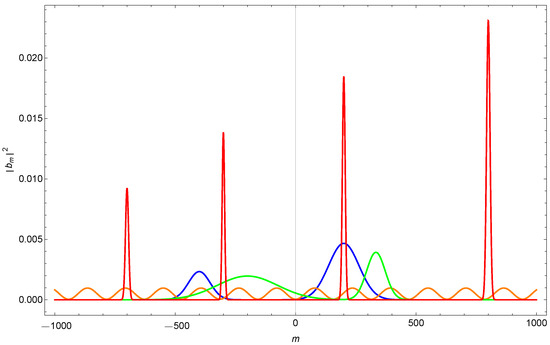
Figure 10. $|b_m{|}^2$, $J_z=m$, for a spin $j=1·{10}^3$ particle in State (83), with four randomly chosen sets of coefficients $\left\{b_m\right\}$.

To discuss the physics of such states, it is useful to recall the so-called Born–Einstein dispute (see, e.g., [34]). Einstein strongly rebuked the idea of Born that the absence of quantum diffusion should be sufficient to explain the classical nature (the unique trajectory) of a macroscopic body, by saying that doubly or multiply split wave packets, with their centers separated by a macroscopic distance, are allowed by the Schrödinger equations, even for a macroscopic particle. Such a split wave function is certainly non-classical.

The missing piece for solving this apparent puzzle turns out to be the temperature [25]. Even though at exceptionally low temperatures such a state is certainly possible, this is not so at finite temperatures. Emission of photons and the ensuing self-decoherence (in the case of an isolated body with finite body temperatures) [25] or an environment-induced decoherence (for an open system) [34,35,36] makes a split system a mixture (a mixed state) essentially instantaneously. Also, they cannot be prepared experimentally, e.g., by passage through a double slit [25]. A (macroscopic) particle passes either through one or the other slit, due to absence of diffusion and/or due to decoherence. The particle after the passage is behind either one or the other slit, even without any measurement.

The status of general angular momentum states with strong fluctuations, as in (83), is similar to that of Einstein’s macroscopic split wave packet. In the large j limit, a generic large spin state (represented by randomly distributed stars, Figure 3), far from the Bloch state $|j,\mathbf{n}⟩$, necessarily acquires a large space extension under an inhomogeneous magnetic field: a macroscopic quantum state. See Figure 10. But a macroscopic pure quantum state is possible only at an exceedingly low temperature close to $T=0$: otherwise, it is a mixture.

Showing quantitatively how a macroscopically split wave packet becomes a mixed state under an environment-induced decoherence is a complex problem, depending on the details of the environment itself, the temperature, density, pressure, kinds of environment particles, and average density and momentum distribution, the mean de Broglie wave length, etc. It is beyond the scope of the present work to perform such a study. However, a qualitative discussion about how a macroscopically split wave packet becomes a mixture under environment-induced decoherence [34,35,36] (but not classical) has been given in [26] in the case of a spin $\frac{1}{2}$ particle.

To tie up possible loose ends of the discussion, note that a single spin $\frac{1}{2}$ isolated atom in its ground state (a microscopic system) travelling in a good vacuum is effectively a system at $T=0$. Thus the fact that its split wave packets can get separated by a macroscopic distance in an SG process—i.e., its being in a macroscopic quantum state—is perfectly consistent with the general argument above. To realize a macroscopic system composed of many atoms and molecules in a pure quantum state, is another story: it is much more difficult to prepare the necessary low temperatures close to $T=0$ to maintain its pure-state nature. At finite temperatures, a macroscopically split wave packet of such a particle, which might arise under the SG set-up, as in Figure 10, is necessarily an incoherent mixture.

An important point to keep in mind, however, is the following. The fact that a macroscopic quantum state such as the split wave packets of Figure 10 becomes a mixture under the decoherence effects at finite temperatures [34,35,36] does not mean that it becomes classical. Decoherence and classical limits are two distinct phenomena in general [26]. This point can hardly be overemphasized.

What is indeed remarkable, perhaps, is the fact that the angular momentum states of minimum fluctuations—(4), (20), (31), and (32)—though pure, effectively become classical at $j\to \infty$, without the help of any (thermal or environment-induced) decoherence effects, hence independently of the temperatures. This might appear to be in line with the familiar discussion of the semi-classical limit of a (pure-state) wave function in QM at $\hslash \to 0$, but our discussion of the generic large-spin states indicates the presence of a loophole in the argument that only the dimensionless ratio $j/\hslash$ should matter.

8. Conclusions

The observations made in this work render the idea that a spin (or angular momentum) j becomes classical in the limit $j\to \infty$ a more precise one. In particular, we found that the states with minimum fluctuations (20) and the states close to them are to be identified with classical angular-momentum vectors in such a limit and verified their consistency through analyses of SG experiments with the angular-momentum composition rule and with the rotation matrix.

At the same time, our analysis has revealed a subtlety in the quantum–classical correspondence in the large-spin limit in general. It reflects the difference between the spaces of the quantum-mechanical and classical angular momentum states of definite magnitude (${\mathbf{CP}}^{2j}$ and ${\mathbf{CP}}^1\sim S^2$, respectively). It is the angular momentum states of minimum fluctuations, (4), (20), (31), and (32), that naturally and smoothly become classical angular momenta in the $j\to \infty$ limit, independently of the temperatures.

On the other hand, more general, strongly fluctuating angular momentum states belonging to ${\mathbf{CP}}^{2j}$ remain quantum-mechanical even in the $j\to \infty$ limit. They can stay pure quantum states only at exceedingly low temperatures, and isolated. The reason is that in the $j\to \infty$ limit such a state necessarily involves a large space extension, in one way or another. A macroscopic system is in a mixed state at finite temperatures [25,34,35,36,37]. No macroscopically split pure wave packets in a SG setting survive decoherence. At the same time, as pointed out in [26], a macroscopic quantum state that becomes a mixture due to decoherence remains a mixed quantum state. Decoherence in itself does not render the system involved classical, contrary to such an idea sometimes expressed in the literature [35,37].

The idea that a large spin is made of many spin-$\frac{1}{2}$ particles turns out to be quite a useful one both mathematically and physically, as we saw in several occasions. The entire theory of angular momentum can indeed be reconstructed this way as shown by Schwinger [27], and it helps to understand certain formulas easily. It is also relevant from the physics point of view, as such a large-angular-momentum system may be regarded as an idealized toy-model version of a macroscopic body made of many atoms and molecules (spins). Seen this way, the sharp spike of the SG projection of the state $|j,\mathbf{n}⟩$ in the narrow region around $J_z=jcos\theta$ we have observed, such as in Figure 5 and Figure 6, can be interpreted as the result of a large number of microscopic states of atoms (spins) accumulating to give such a value of $J_z$. (The suppression of the fluctuations of angular momentum components we observed in this paper in the $j\to \infty$ limit is somewhat analogous to the “$\sqrt{n}$ law” invoked by Schrödinger [38] to explain the general exactness (classicality) of laws of the macroscopic world based on statistical mechanics, although, here, the relevant fluctuations are quantum-mechanical ones. This being so, let us not forget that the deepest insight of Schrödinger in his book was that many biological processes such as mutation, reproduction, and inheritance involve quantum mechanics in essential ways).

Nevertheless, our discussion is really about the quantum and classical properties of a single large spin, and do not concern the thermodynamical, statistical, or other physical properties of realistic many-body systems, as in [6,7]. And in spite of inevitable partial overlaps with numerous observations made in the literature [1,2,3,4,5,6,7,8,9,10,11,12,13,14,15,16,17,18,19,20,21,22,23,24], our careful observations about how the particular class of large-momentum (spin) states becomes classical in the limit $j\to \infty$ independently of temperature, whereas generic large j states remain quantum mechanical in the same limit, as illustrated in Section 2, Section 5, and Section 7, are, to the best of our knowledge, new.

References

- Brussard, P.J.; Tolhoek, H.A. Classical limits of Clebsch-Gordan coefficients, Racah coefficients and (φ,ϑ,ψ)-functions. Physica 1957, 23, 955. [Google Scholar] [CrossRef]
- Barut, A.O.; Dilley, J. Behavior of the Scattering Amplitude for Large Angular Momentum. J. Math. Phys. 1963, 4, 1401. [Google Scholar] [CrossRef]
- Cederberg, J.W.; Ramsey, N.F. Magnetic Resonance with Large Angular Momentum. Phys. Rev. 1964, 135, A39. [Google Scholar] [CrossRef]
- Newton, R.G.; Young, B.-l. Measurability of the spin density matrix. Ann. Phys. 1968, 49, 393. [Google Scholar] [CrossRef]
- Radcliffe, J.M. Some properties of coherent spin states. J. Phys. A Gen. Phys. 1971, 4, 313–323. [Google Scholar] [CrossRef]
- Arecchi, F.T.; Courtens, E.; Gilmore, R.; Thomas, H. Atomic Coherence States in Quantum Optics. Phys. Rev. A 1972, 6, 2211. [Google Scholar] [CrossRef]
- Lieb, E.H. The Classical Limit of Quantum Spin Systems. Commun. Math. Phys. 1973, 31, 327. [Google Scholar] [CrossRef]
- Wu, H.C. Bosons with large angular momentum and rotation of even-even nuclei. Phys. Lett. B 1982, 110, 1–6. [Google Scholar] [CrossRef]
- Wodkiewicz, K.; Eberly, J.H. Coherent states, squeezed fluctuations, and the SU(2) am SU(1,1) groups in quantum-optics applications. J. Opt. Soc. Am. B 1985, 2, 458–466. [Google Scholar] [CrossRef]
- Allen, L.; Beijersbergen, M.W.; Spreeuw, R.J.C.; Woerdman, J.P. Orbital angular momentum of light and the transformation of Laguerre-Gaussian laser modes. Phys. Rev. A 1992, 45, 8185. [Google Scholar] [CrossRef]
- Puri, R.R. Coherent and squeezed states on physical basis. Pramana—J. Phys. 1997, 48, 787. [Google Scholar] [CrossRef]
- Aravind, P.K. Spin coherent states as anticipators of the geometric phase. Am. J. Phys. 1999, 67, 899. [Google Scholar] [CrossRef]
- Klose, G.; Smith, G.; Jessen, P.S. Measuring the Quantum State of a Large Angular Momentum. Phys. Rev. Lett. 2001, 86, 4721. [Google Scholar] [CrossRef] [PubMed]
- Imamura, Y. Large angular momentum closed strings colliding with D-branes. J. High Energy Phys. 2002, 6, 5. [Google Scholar]
- Livine, E.R.; Speziale, S. New spinfoam vertex for quantum gravity. Phys. Rev. D 2007, 76, 084028. [Google Scholar] [CrossRef]
- Anderson, R.W.; Aquilanti, V.; da Silva Ferreira, C. Exact computation and large angular momentum asymptotics of 3nj symbols: Semiclassical disentangling of spin networks. J. Chem. Phys. 2008, 129, 161101. [Google Scholar] [CrossRef]
- Dajka, J. Disentanglement of Qubits in Classical Limit of Interaction. Int. J. Theor. Phys. 2014, 53, 870. [Google Scholar] [CrossRef]
- Kovacs, S.; Sato, Y.; Shimada, H. Membranes from monopole operators in ABJM theory: Large angular momentum and M-theoretic AdS4/CFT3. Prog. Theor. Exp. Phys. 2014, 9, 093B01. [Google Scholar] [CrossRef]
- Loh, Y.L.; Kim, M. Visualizing spin states using the spin coherent state representation. Am. J. Phys. 2015, 83, 30. [Google Scholar] [CrossRef]
- Byrnes, T.; Rosseau, D.; Khosla, M.; Pyrkov, A.; Thomasen, A.; Mukai, T.; Koyama, S.; Abdelrahman, A.; Ilo-Okeke, E. Macroscopic quantum information processing using spin coherent states. Opt. Commun. 2015, 337, 102–109. [Google Scholar] [CrossRef]
- Chen, Y.Y.; Li, J.X.; Hatsagortsyan, K.Z.; Keitel, C.H. γ-Ray Beams with Large Orbital Angular Momentum via Nonlinear Compton Scattering with Radiation Reaction. Phys. Rev. Lett. 2018, 121, 074801. [Google Scholar] [CrossRef] [PubMed]
- Kus, M.; Mostowski, J.; Pietraszewicz, J. Classical limit of entangled states of two angular momenta. Phys. Rev. A 2019, 99, 052112. [Google Scholar] [CrossRef]
- Braccini, L.; Schut, M.; Serafini, A.; Mazumdar, A.; Bose, S. Large Spin Stern-Gerlach Interferometry for Gravitational Entanglement. arXiv 2023, arXiv:2312.05170. [Google Scholar] [CrossRef]
- Corso, P.P.; Cricchio, D.; Fiordilino, E. Large Angular Momentum States in a Graphene Film. Physics 2024, 6, 317. [Google Scholar] [CrossRef]
- Konishi, K. Newton’s equations from quantum mechanics for a macroscopic body in the vacuum. Int. J. Mod. Phys. A 2023, 38, 2350080. [Google Scholar] [CrossRef]
- Konishi, K.; Elze, H.T. The Quantum Ratio. Symmetry 2024, 169, 427. [Google Scholar] [CrossRef]
- Schwinger, J. On Angular Momentum. In A Quantum Legacy; World Scientific Series in 20th Century Physics; A reproduction of a book chapter from Biedenharn, L.C.; van Dam, H. Angular Momentum in Quantum Physics; Academic Press: New York, NY, USA, 1965. https://doi.org/10.2172/4389568; World Scientific: Singapore, 2000; pp. 173–223. [Google Scholar] [CrossRef]
- Bengtsson, I.; Zyczkowski, K. Geometry of Quantum States: An Introduction to Quantum Entanglement; Cambridge University Press: Cambridge, UK, 2006. [Google Scholar] [CrossRef]
- Dubrovin, B.A.; Novikov, S.P.; Fomenko, A.T. Modern Geometry—Methods and Applications. Part II: The Geometry and Topology of Manifolds; Graduate Texts in Mathematics; Springer: New York, NY, USA, 1985. [Google Scholar] [CrossRef]
- Gerlach, W.; Stern, O. Der experimentelle Nachweis der Richtungsquantelung im Magnetfeld. Z. Phys. 1922, 9, 349. [Google Scholar] [CrossRef]
- Alstrøm, P.; Hjorth, P.; Mattuck, R. Paradox in the classical treatment of the Stern-Gerlach experiment. Am. J. Phys. 1982, 50, 697. [Google Scholar] [CrossRef]
- Platt, D.E. A modern analysis of the Stern-Gerlach experiment. Am. J. Phys. 1992, 60, 306. [Google Scholar] [CrossRef]
- Konishi, K. On the negative-result experiments in quantum mechanics. Entropy 2024, 26, 958. [Google Scholar] [CrossRef]
- Joos, E.; Zeh, H.D. The emergence of classical properties through interaction with the environment. Z. Phys. B 1985, 59, 223. [Google Scholar] [CrossRef]
- Zurek, W.H. Decoherence and the Transition from Quantum to Classical. Phys. Today 1991, 44, 36. [Google Scholar] [CrossRef]
- Tegmark, M. Apparent wave function collapse caused by scattering. Found. Phys. Lett. 1993, 6, 571. [Google Scholar] [CrossRef]
- Joos, E.; Zeh, H.D.; Kiefer, C.; Giulini, D.; Kupsch, J.; Stamatescu, I.O. Decoherence and the Appearance of a Classical World in Quantum Theory; Springer: Berlin/Heidelberg, Germany, 2003. [Google Scholar] [CrossRef]
- Schrödinger, E. What Is Life? Cambridge University Press: Cambridge, UK, 1944. [Google Scholar] [CrossRef]
- Kwiat, P.G.; Steinberg, A.M.; Chiao, R.Y. Observation of a “quantum eraser”: A revival of coherence in a two-photon interference experiment. Phys. Rev. A 1992, 45, 7729. [Google Scholar] [CrossRef]
Disclaimer/Publisher’s Note: The statements, opinions and data contained in all publications are solely those of the individual author(s) and contributor(s) and not of MDPI and/or the editor(s). MDPI and/or the editor(s) disclaim responsibility for any injury to people or property resulting from any ideas, methods, instructions or products referred to in the content. |
© 2025 by the authors. Licensee MDPI, Basel, Switzerland. This article is an open access article distributed under the terms and conditions of the Creative Commons Attribution (CC BY) license (https://creativecommons.org/licenses/by/4.0/).