An Effective Multi-Revolution Lambert Solver Based on Elementary Calculus

Abstract

Multi-revolution Lambert solvers are intended to find the elliptic transfer orbits that are traveled multiple times and connect two specified positions in prescribed time, under the assumption of considering natural (Keplerian) orbital motion in the presence of a single attracting body. This study proposes and tests a new, effective multi-revolution Lambert solver that employs the initial true anomaly, which identifies the initial position along the transfer ellipse, as the unknown variable. The related search interval is identified through closed-form expressions for upper and lower bounds. A simple numerical algorithm is developed and employed over the entire search interval to detect all Lambert solutions. The new multi-revolution solver proposed in this work is simple to understand and easy to implement and is successfully tested in several challenging scenarios (corresponding to some pathological cases reported in the recent scientific literature), as well as for the study of Earth–Mars interplanetary transfers. Comparison with alternative, up-to-date techniques points out that the new approach at hand is able to detect all the feasible transfer ellipses, in all cases, with very satisfactory accuracy in terms of final position error, even in challenging scenarios that include a huge number of revolutions or near-antipodal terminal positions.

1. Introduction

In orbital mechanics, the two-point boundary value problem for natural motion in the presence of a single attracting body is referred to as the Lambert problem. This is solved by determining the conic that connects two terminal (i.e., initial and final) positions in space in prescribed time.

The problem was originally formulated by Lagrange [1] and Gauss [2], with the initial purpose of precise orbit determination of recently-discovered celestial bodies, such as Ceres. In the 20th century, its relevance in astrodynamics applications was widely recognized, with particular reference to interception and rendezvous, orbit determination (including space debris correlation), orbit design in planetary and interplanetary mission contexts, and missile guidance. In the scientific literature, a vast amount of contributions were devoted to the analysis and solution of the Lambert problem. In most formulations, finding the conic arc of interest implies solving numerically a single trascendental equation in a single unknown. In a recent survey [3], a significant variety of methods were classified on the basis of the unknown variable, namely, (a) semimajor axis [4,5,6,7,8], (b) semilatus rectum [9,10,11], (c) eccentricity vector [12,13,14,15,16], (d) Kustaanheimo–Stiefel (K-S) regularized coordinates [17,18,19], and (e) universal variables [9,20,21,22,23,24,25,26,27,28,29,30]. The usefulness and versatility of techniques able to deal with all types of conics pushed the development of universal approaches [9,19,22,23,31,32,33,34,35,36,37]. In particular, Gooding’s technique [22], based on the preceding contribution by Lancaster and Blanchard [34], is widely known to be highly efficient and robust, for both elliptic and hyperbolic trajectories.

Several methods were extended to multi-revolution scenarios, which explicitly refer to closed trajectories, i.e., elliptic orbits repeatedly traveled multiple times. Battin [32] provides a detailed analysis on the multi-revolution Lambert problem, as well as Ochoa and Prussing [7,38]. For specified boundary positions, transfer time $\Delta t$, and number of revolutions $n_{rev}$$(\ge 1)$, the Lambert problem admits zero, two, or four solutions. In fact, for a specific value of $n_{rev}$, the minimum time $\Delta t_{min}$ can be identified. Three cases can occur:

• if $\Delta t<\Delta t_{min}$, then no solution exists;
• if $\Delta t=\Delta t_{min}$, then two solutions exist, termed direct and retrograde ellipses;
• if $\Delta t>\Delta t_{min}$, then four solutions exists, i.e., two direct ellipses and two retrograde ellipses.

In his recent work [39], Russell identifies four particularly challenging scenarios for multi-revolution Lambert solvers, namely, (1) flight time too large, (2) flight time too close to $\Delta t_{min}$, (3) near-antipodal terminal positions (i.e., transfer angle close to 180°), and (4) near full revolution (i.e., near-identical terminal positions). Significant efforts were devoted to increasing the effectiveness of algorithms with reference to the preceding pathological cases. Izzo [23] improved the Gooding’s method in terms of computational efficiency, while Arora and Russell proposed, developed, and refined an effective universal formulation based on the vercosine function [27,39,40]. Most recently, to solve the problem at hand, Negrete and Abdelkhalik [41] have introduced contour integrals in the complex domain, while McElreath et al. [42] have employed matrix exponential solutions to the Sundman transform, to evaluate the transfer time equation through exponential functions, with application in scenarios including up to 100,000 revolutions.

Desirable properties of solution methods for multi-revolution problems are (i) simplicity of the formulation, with regard to both the physical (or geometric) interpretation of the variables and ease of implementation, (ii) robustness, i.e., capability of detecting all four transfer ellipses, (iii) accuracy in determining the orbit elements corresponding to negligible displacements of the terminal positions from the prescribed boundary points, and (iv) computational efficiency.

Based on elementary calculus, the work that follows is intended to propose and test an effective multi-revolution Lambert solver that employs the initial true anomaly, associated with the initial position along the transfer ellipse, as the unknown variable. More specifically, this research has the following objectives: (a) develop a general framework for the description of multi-revolution orbit transfers between two positions in given time, in which the initial true anomaly represents the only unknown, i.e., the fundamental quantity to determine numerically; (b) identify the upper and lower bounds of the search space for the latter variable; (c) obtain the explicit expression of the fundamental solving equation, with initial true anomaly as the unknown parameter; (d) analyze all special cases that can occur, including circular transfer arc and collinear terminal positions; (e) design and develop a simple and effective algorithm for the numerical solution of the fundamental equation; (f) test the new multi-revolution Lambert solver at hand in some challenging scenarios, corresponding to the pathological cases identified by Russell [39]; (g) compare the numerical results with two well-established up-to-date alternative methodologies, namely the Oldenhuis implementation [43] and the very recent approach proposed by McElreath et al. [42]; (h) show the application of the new solver in the study of Earth–Mars interplanetary transfers. Because only orbit elements and well-established relations of Keplerian motion are utilized, the technique proposed in this research, termed the ITA (initial-true-anomaly)-method henceforth, is simple to understand and straightforward to implement. No contour integral, series expansions, or non-intuitive variable as the unknown are introduced. Instead, the problem is shown to be tractable and solvable with an elementary numerical technique, i.e., regula falsi, that is well suited to detect all solutions in a well-defined search interval. Other than simplicity, which is a distinguishing feature of the ITA-method, comparison with alternative techniques focuses on (ii) robustness and (iii) accuracy, while a comparative analysis on computational efficiency is out of the scope of this work. The final intent is in showing that the simple, new Lambert solver proposed in this study can represent a valuable option, also in the presence of very large number of revolutions or near-antipodal terminal positions.

2. Formulation of the Problem

The Lambert problem is formulated in the general framework of Keplerian motion, which describes the natural dynamics of a point mass m, subject to the gravitational attraction of a single massive attracting body, with mass M. In astrodynamics, the point-mass model is useful to describe the orbit dynamics of a spacecraft, which does not affect the attracting body because $M\gg m$. The Lambert problem consists in determining the conic arc that connects two successive positions of the spacecraft, denoted with ${\overrightarrow{\mathit{r}}}_0$ and ${\overrightarrow{\mathit{r}}}_f$, in a specified time of flight $\Delta t=t_f-t_0$.

As a preliminary step needed to describe three-dimensional Keplerian motion, an inertial reference frame is introduced, with origin at the center of the attracting body and associated with the right-hand sequence of unit vectors. $({\widehat{\mathbf{c}}}_1,{\widehat{\mathbf{c}}}_2,{\widehat{\mathbf{c}}}_3)$. Vector ${\widehat{\mathbf{c}}}_3$ is aligned with the rotation axis of the central body, while $({\widehat{\mathbf{c}}}_1,{\widehat{\mathbf{c}}}_2)$ span the equatorial plane. As a special case, the Earth-Centered Inertial (ECI) frame refers to the Earth, and has axis ${\widehat{\mathbf{c}}}_1$ corresponding to the intersection of the equatorial plane with the ecliptic plane at a reference epoch.

Orbital motion is described in terms of the spacecraft instantaneous position and velocity, $\overrightarrow{\mathit{r}}$ and $\overrightarrow{\mathit{v}}$. The specific angular momentum $\overrightarrow{\mathit{h}}$, given by $\overrightarrow{\mathit{h}}=\overrightarrow{\mathit{r}}\times \overrightarrow{\mathit{v}}$, is an integral of the dynamical system, and identifies the (invariant) plane where Keplerian motion takes place. The related unit vector $\widehat{\mathbf{h}}$, in conjunction with the radial and horizontal unit vectors $\widehat{\mathbf{r}}$ and $\widehat{\mathsf{\theta }}$, forms the right-hand triad $(\widehat{\mathbf{r}},\widehat{\mathsf{\theta }},\widehat{\mathbf{h}})$, associated with the rotating local vertical local horizontal (LVLH) frame. If matrix ${\mathbf{R}}_j\left(\alpha \right)$ represents the counterclockwise elementary rotation about axis j by angle $\alpha$, the LVLH-frame is obtained from the inertial frame through the following sequence [44]:

$${\left[\widehat{\mathbf{r}}\widehat{\mathsf{\theta }}\widehat{\mathbf{h}}\right]}^{\top }={\mathbf{R}}_3\left({\theta }_t\right){\mathbf{R}}_1\left(i\right){\mathbf{R}}_3(\Omega ){\left[{\widehat{\mathbf{c}}}_1{\widehat{\mathbf{c}}}_2{\widehat{\mathbf{c}}}_3\right]}^{\top }=:\mathbf{M}(i,\Omega ,{\theta }_t){\left[{\widehat{\mathbf{c}}}_1{\widehat{\mathbf{c}}}_2{\widehat{\mathbf{c}}}_3\right]}^{\top }$$

(1)

where symbols $\Omega$ and i denote the right ascension of the ascending node (RAAN) and inclination, respectively, whereas

$${\theta }_t=\omega +{\theta }_{\ast }$$

(2)

is the argument of latitude, written in terms of the argument of periapse $\omega$ and true anomaly ${\theta }_{\ast }$. It is worth remarkng that matrix $\mathbf{M}$ contains the components of the three unit vectors $(\widehat{\mathbf{r}},\widehat{\mathsf{\theta }},\widehat{\mathbf{h}})$ in the inertial frame. Its explicit expression is reported in [44]. The Keplerian conic that connects the two terminal positions is identified by the five constant orbit elements $\{a,e,i,\Omega ,\omega \}$, with a and e denoting the orbit semimajor axis and eccentricity, while the two terminal positions correspond to two distinct values of the true anomaly, ${\theta }_{\ast ,0}$ and ${\theta }_{\ast ,f}$. A Lambert solver has the final goal of determining all the transfer paths, with the respective values of $\{a,e,i,\Omega ,\omega \}$, ${\theta }_{\ast ,0}$, and ${\theta }_{\ast ,f}$, compatible with the prescribed transfer time $\Delta t$.

3. Analysis and Methodology

This study focuses on multi-revolution Lambert solutions, i.e., elliptic orbits that connect the two given positions, after completing an integer number $n_{rev}$ of revolutions about the attracting body. Previous research showed that up to four distinct solutions may exist [7]. This work is intended to introduce a new methodology able to identify these solutions, if existing, in particularly challenging cases, such as those described in Section 1.

3.1. Transfer Ellipse

As a preliminary step, the orbit plane of the transfer ellipse can be identified. Because both ${\overrightarrow{\mathit{r}}}_0$ and ${\overrightarrow{\mathit{r}}}_f$ correspond to two positions along the transfer path, the orbit plane is orthogonal to the direction identified by $\overrightarrow{\mathit{n}}:={\overrightarrow{\mathit{r}}}_0\times {\overrightarrow{\mathit{r}}}_f$, provided that the two position vectors are not aligned. Two distinct options exist for the unit vector $\widehat{\mathbf{h}}$, aligned with the angular momentum of the transfer ellipse:

$$\left(\mathrm{A}\right){\widehat{\mathbf{h}}}^{\left(A\right)}={\displaystyle \frac{\overrightarrow{\mathit{n}}}{|\overrightarrow{\mathit{n}}|}}\mathrm{or}\left(\mathrm{B}\right){\widehat{\mathbf{h}}}^{\left(B\right)}=-{\displaystyle \frac{\overrightarrow{\mathit{n}}}{|\overrightarrow{\mathit{n}}|}}$$

(3)

If the position vectors are specified in terms of their components in the inertial frame, then ${\widehat{\mathbf{h}}}^{(A/B)}$ can be obtained through Equation (3). This allows finding the three components of ${\widehat{\mathbf{h}}}^{(A/B)}$ in the inertial frame, denoted with $(h_1,h_2,h_3)$ and coinciding with the elements $m_{3,1}$, $m_{3,2}$, and $m_{3,3}$ of matrix $\mathbf{M}$ (cf. Equation (1)):

$$m_{3,1}=sinisin\Omega =h_1{m}_{3,2}=-sinicos\Omega =h_2{m}_{3,3}=cosi=h_3$$

(4)

The preceding relations lead to obtaining two possible pairs of values for $\{i,\Omega \}$, denoted with $\{i^{\left(A\right)},{\Omega }^{\left(A\right)}\}$ and $\{i^{\left(B\right)},{\Omega }^{\left(B\right)}\}$, under the assumption that $sini\ne 0$. If either $i=0$ or $i=\pi$, an auxiliary inertial frame is introduced, as discussed in Appendix A.

Because ${\widehat{\mathbf{r}}}_0$ and ${\widehat{\mathbf{h}}}^{(A/B)}$ are known at $t_0$, unit vector ${\widehat{\mathsf{\theta }}}_0^{(A/B)}$ can be found, with components denoted with $({\theta }_{0,1}^{(A/B)},{\theta }_{0,2}^{(A/B)},{\theta }_{0,3}^{(A/B)})$. Let $r_{0,3}$ denote the third component of ${\overrightarrow{\mathit{r}}}_0$ in the inertial frame. The argument of latitude at $t_0$, ${\theta }_{t,0}^{(A/B)}$, can be found from $r_{0,3}$ and ${\theta }_{0,3}^{(A/B)}$,

$$m_{1,3}=r_{0,3}=sinisin{\theta }_{t,0}^{(A/B)}\mathrm{and}{m}_{2,3}={\theta }_{0,3}^{(A/B)}=sinicos{\theta }_{t,0}^{(A/B)}$$

(5)

Similar steps lead to finding ${\theta }_{t,f}^{(A/B)}$ from $r_{f,3}$ and ${\theta }_{f,3}^{(A/B)}$. Due to the definition of argument of latitude,

$$\Delta {\theta }_t^{(A/B)}:={\theta }_{t,f}^{(A/B)}-{\theta }_{t,0}^{(A/B)}={\theta }_{\ast ,f}^{(A/B)}-{\theta }_{\ast ,0}^{(A/B)}$$

(6)

Then, the polar equation of the ellipse [45] can be used at the two terminal points,

$$r_0={\displaystyle \frac{p^{(A/B)}}{1+e^{(A/B)}cos{\theta }_{\ast ,0}^{(A/B)}}}\mathrm{and}{r}_f={\displaystyle \frac{p^{(A/B)}}{1+e^{(A/B)}cos{\theta }_{\ast ,f}^{(A/B)}}}$$

(7)

where $p^{(A/B)}$ represents the semilatus rectum, ${\theta }_{\ast ,f}^{(A/B)}={\theta }_{\ast ,0}^{(A/B)}+\Delta {\theta }_t^{(A/B)}$ (from Equation (6)), whereas $r_0=\left|{\overrightarrow{\mathit{r}}}_0\right|$ and $r_f=\left|{\overrightarrow{\mathit{r}}}_f\right|$. Combination of the preceding two relations leads to

$$e^{(A/B)}={\displaystyle \frac{r_f-r_0}{r_{0}cos{\theta }_{\ast ,0}^{(A/B)}-r_{f}cos\left({\theta }_{\ast ,0}^{(A/B)}+\Delta {\theta }_t^{(A/B)}\right)}}$$

(8)

under the assumption that $r_0\ne r_f$ (the case $r_0=r_f$ is addressed in Section 3.4). The semimajor axis is found from the polar equation again,

$$a^{(A/B)}={\displaystyle \frac{r_0\left(1+e^{(A/B)}cos{\theta }_{\ast ,0}^{(A/B)}\right)}{1-{\left(e^{(A/B)}\right)}^2}}$$

(9)

with $e^{(A/B)}$ written in terms of the unknown ${\theta }_{\ast ,0}^{(A/B)}$ (cf. Equation (8)). Finally, the argument of periapse is also written as a function of ${\theta }_{\ast ,0}^{(A/B)}$,

$${\omega }^{(A/B)}={\theta }_{t,0}^{(A/B)}-{\theta }_{\ast ,0}^{(A/B)}$$

(10)

It is worth noticing that several variables (with superscript ^(A/B)) correspond to the two options (A) and (B) of Equation (3), associated with opposite directions of the angular momentum.

In the special case that position vectors ${\overrightarrow{\mathit{r}}}_0$ and ${\overrightarrow{\mathit{r}}}_f$ are aligned, then a unique orbit plane cannot be identified, as infinite orbit planes contain the line associated with ${\overrightarrow{\mathit{r}}}_0$ and ${\overrightarrow{\mathit{r}}}_f$. However, once a specific orbit plane is selected, then the four solutions reduce to two distinct ellipses [39], with opposite direction of their respective angular momentum. In this limiting case, starting from the initial orbit, the choice of a specific plane (and the resulting pair of ellipses) can be driven by considerations of a practical nature, such as the minimization of the propellant needed to enter the transfer path (chosen between the two available ellipses) and exit the transfer trajectory (to enter the final orbit).

A very special case occurs if the initial and final position coincide, i.e., ${\overrightarrow{\mathit{r}}}_0\equiv {\overrightarrow{\mathit{r}}}_f$, and admits again an infinite number of solutions. In fact, the transfer plane is not uniquely defined, in the sense that all the orbit planes that contain the two coinciding vectors ${\overrightarrow{\mathit{r}}}_0$ and ${\overrightarrow{\mathit{r}}}_f$ are admissible. Moreover, the transfer time and number of revolutions lead to finding the semimajor axis a of the transfer ellipse. However, all ellipses that satisfy the polar equation are admissible, and this implies that an entire family of solutions can be identified, i.e., those that satisfy the following relation:

$$r_0=r_f={\displaystyle \frac{a(1-e^2)}{1+ecos{\theta }_{\ast ,0}}}$$

(11)

Equation (11) establishes a direct relation between e and ${\theta }_{\ast ,0}$ of the transfer ellipse, and definitely shows that infinite solutions exist, even after selecting a specific orbit plane among all feasible ones.

With the exception of the previously mentioned special cases, the preceding steps are useful to express all the orbit elements $\{a,e,i,\Omega ,\omega \}$, together with ${\theta }_{\ast ,f}$, as functions of ${\theta }_{\ast ,0}$ (at most). The next subsection addresses the derivation of the solving equation for ${\theta }_{\ast ,0}$, regarded as the only remaining unknown parameter for the problem at hand.

3.2. Fundamental Equation

The fundamental equation derives directly from the Kepler’s law, which relates the time of flight to the eccentric anomalies at the terminal points of an elliptic orbit. Omitting superscripts for the sake of simplicity, the Kepler’s equation for the multi-revolution problem is

$$(E_f-esin{E}_f)-(E_0-esin{E}_0)+2\pi n_{rev}=\sqrt{{\displaystyle \frac{\mu }{a^3}}}\Delta t,$$

(12)

In the preceding expression, $E_0$ and $E_f$ represent the eccentric anomalies corresponding to ${\theta }_{\ast ,0}$ and ${\theta }_{\ast ,f}$, respectively. They are given by

$$E_0=2{tan}^{-1}\left[\sqrt{{\displaystyle \frac{1-e}{1+e}}}tan{\displaystyle \frac{{\theta }_{\ast ,0}}{2}}\right],E_f=2{tan}^{-1}\left[\sqrt{{\displaystyle \frac{1-e}{1+e}}}tan{\displaystyle \frac{{\theta }_{\ast ,f}}{2}}\right].$$

(13)

while

$$\begin{array}{c}\hfill sin{E}_0={\displaystyle \frac{\sqrt{1-e^2}}{1+ecos{\theta }_{\ast ,0}}}sin{\theta }_{\ast ,0},sin{E}_f={\displaystyle \frac{\sqrt{1-e^2}}{1+ecos{\theta }_{\ast ,f}}}sin{\theta }_{\ast ,f}.\end{array}$$

(14)

The term $(E_f-E_0)$ that appears in Equation (12) must be properly constrained to the interval $[0,2\pi [$, in order that the correct solution associated with $n_{rev}$ complete revolutions be computed.

Equation (12) involves a single unknown, i.e., the initial true anomaly ${\theta }_{\ast ,0}$, because all the remaining terms can be expressed as functions of ${\theta }_{\ast ,0}$:

• ${\theta }_{\ast ,f}$, through Equation (6);
• e, through Equation (8);
• $E_0$ and $E_f$ and the respective sin functions, through Equations (13) and (14), also using the relations at the preceding points;
• a through Equation (9).

Based on the preceding points and relations and omitting intermediate steps for the sake of brevity, the explicit-form fundamental equation contains a single unknown variable, i.e., the initial true anomaly ${\theta }_{\ast ,0}$, and is given by

$$\begin{array}{cc}\hfill & mod\{2{tan}^{-1}\left[\sqrt{{\displaystyle \frac{r_0(c_0+1)-r_f(c_f+1)}{r_0(c_0-1)-r_f(c_f-1)}}}tan{\displaystyle \frac{{\theta }_{\ast ,f}}{2}}\right]\hfill \\ \hfill & -2{tan}^{-1}\left[\sqrt{{\displaystyle \frac{r_0(c_0+1)-r_f(c_f+1)}{r_0(c_0-1)-r_f(c_f-1)}}}tan{\displaystyle \frac{{\theta }_{\ast ,0}}{2}}\right],2\pi \}\hfill \\ \hfill & +{\displaystyle \frac{(r_f-r_0)(s_0{r}_0-s_f{r}_f)}{|r_0{c}_0-r_f{c}_f|r_0{r}_f(c_0-c_f)}}\sqrt{2r_0{r}_f(1-c_0{c}_f)-r_0^2{s}_0^2-r_f^2{s}_f^2}\hfill \\ \hfill & +2\pi n_{rev}-\Delta t\sqrt{{\displaystyle \frac{\mu {[2r_0{r}_f(1-c_0{c}_f)-r_0^2{s}_0^2-r_f^2{s}_f^2]}^3}{r_0^3{r}_f^3{(c_0-c_f)}^3{(r_0{c}_0-r_f{c}_f)}^3}}}=0\hfill \end{array}$$

(15)

where the mod function has an angular displacement as its argument, and translates it to the interval $[0,2\pi [$, while ${\theta }_{\ast ,f}={\theta }_{\ast ,0}+\Delta {\theta }_t$, $c_0:=cos{\theta }_{\ast ,0}$, $c_f:=cos({\theta }_{\ast ,0}+\Delta {\theta }_t)$, $s_0:=sin{\theta }_{\ast ,0}$, and $s_f:=sin({\theta }_{\ast ,0}+\Delta {\theta }_t)$. The equality $c_0=c_f$ implies $r_0=r_f$, which is treated as a separate case (cf. Section 3.4). Therefore, Equation (15) implicitly assumes $c_0\ne c_f$, which also implies $r_0{c}_0\ne r_f{c}_f$.

It is worth remarking that orbit elements $\{i,\Omega \}$, as well as $\Delta {\theta }_t$, are independent of ${\theta }_{\ast ,0}$, and attainable through Equations (4) and (6). All the remaining quantities of interest can be calculated, once all the values of ${\theta }_{\ast ,0}$ that solve Equation (15) are found. To do this, the search interval for the initial true anomaly is to be identified first.

3.3. Search Interval for the Initial True Anomaly

The initial true anomaly is to be sought in an interval such that two basic conditions are met,

$$0\le e={\displaystyle \frac{r_f-r_0}{r_{0}cos{\theta }_{\ast ,0}-r_{f}cos({\theta }_{\ast ,0}+\Delta {\theta }_t)}}<1$$

(16)

$$a={\displaystyle \frac{r_0(1+ecos{\theta }_{\ast ,0})}{1-e^2}}>0$$

(17)

However, the latter inequality is certainly satisfied if Equation (16) holds. Therefore, only the double inequality contained in Equation (16) is to be investigated. Two different cases are considered.

Case 1: $r_0<r_f$. Because $r_0<r_f$, the inequality $e\ge 0$ yields

$$(r_0-r_{f}cos\Delta {\theta }_t)cos{\theta }_{\ast ,0}+r_{f}sin\Delta {\theta }_{t}sin{\theta }_{\ast ,0}>0$$

(18)

Letting

$$k_1:=(r_0-r_{f}cos\Delta {\theta }_t)\mathrm{and}{k}_2:=r_{f}sin\Delta {\theta }_t$$

(19)

the preceding inequality becomes

$$\sqrt{k_1^2+k_2^2}sin({\theta }_{\ast ,0}+\phi )>0$$

(20)

with

$$sin\phi :={\displaystyle \frac{k_1}{\sqrt{k_1^2+k_2^2}}}\mathrm{and}cos\phi :={\displaystyle \frac{k_2}{\sqrt{k_1^2+k_2^2}}}$$

(21)

Due to Equation (20), the initial true anomaly must be constrained to the following interval:

$$-\phi <{\theta }_{\ast ,0}<\pi -\phi$$

(22)

Because the denominator in Equation (16) is positive, the inequality $e<1$ yields

$$(r_0-r_{f}cos\Delta {\theta }_t)cos{\theta }_{\ast ,0}+r_{f}sin\Delta {\theta }_{t}sin{\theta }_{\ast ,0}>r_f-r_0$$

(23)

Using the preceding definitions of $k_1$, $k_2$, and $\phi$, Equation (23) becomes

$$\sqrt{k_1^2+k_2^2}sin({\theta }_{\ast ,0}+\phi )>r_f-r_0$$

(24)

The triangular inequality allows proving that

$${\displaystyle \frac{|r_f-r_0|}{\sqrt{k_1^2+k_2^2}}}\le 1$$

(25)

because $\sqrt{k_1^2+k_2^2}=\sqrt{r_0^2+r_f^2-2r_0{r}_{f}cos\Delta {\theta }_t}$. As a result, Equation (24) yields

$$\alpha -\phi <{\theta }_{\ast ,0}<\pi -\phi -\alpha$$

(26)

where $\alpha$ denotes the auxiliary angle given by

$$\alpha ={sin}^{-1}{\displaystyle \frac{r_f-r_0}{\sqrt{r_0^2+r_f^2-2r_0{r}_{f}cos\Delta {\theta }_t}}}$$

(27)

As the latter inequality is more restrictive than that in Equations (22), Equation (26) represents the search interval for Case 1.

Case 2: $r_0>r_f$. Because $r_0>r_f$, the inequality $e>0$ yields

$$(r_0-r_{f}cos\Delta {\theta }_t)cos{\theta }_{\ast ,0}+r_{f}sin\Delta {\theta }_{t}sin{\theta }_{\ast ,0}<0$$

(28)

Using the preceding definitions of $k_1$, $k_2$, and $\phi$, Equation (28) becomes

$$\sqrt{k_1^2+k_2^2}sin({\theta }_{\ast ,0}+\phi )<0$$

(29)

and the true anomaly must be constrained to the following interval:

$$\pi -\phi <{\theta }_{\ast ,0}<2\pi -\phi$$

(30)

Because the denominator in Equation (16) is negative, the inequality $e<1$ yields

$$(r_0-r_{f}cos\Delta {\theta }_t)cos{\theta }_{\ast ,0}+r_{f}sin\Delta {\theta }_{t}sin{\theta }_{\ast ,0}<r_f-r_0$$

(31)

Using the preceding definitions of $k_1$, $k_2$, and $\phi$, Equation (31) becomes

$$\sqrt{k_1^2+k_2^2}sin({\theta }_{\ast ,0}+\phi )<r_f-r_0$$

(32)

The latter inequality yields

$$\pi -\phi -\alpha <{\theta }_{\ast ,0}<2\pi -\phi +\alpha$$

(33)

where $\alpha$ is given by Equation (27). Because the latter inequality is more restrictive than that in Equations (30), Equation (33) represents the search interval for Case 2.

3.4. Special Case $(r_0=r_f)$

The previous Equation (7) leads to Equation (8), under the assumption that $r_0\ne r_f$. Instead, if $r_0=r_f$, then Equation (7) yields the following:

$$r_{0}e(cos{\theta }_{\ast ,f}-cos{\theta }_{\ast ,0})=0$$

(34)

Because $r_0\ne 0$, the preceding relation admits two solutions: (a) $e=0$ and (b) $cos{\theta }_{\ast ,f}=cos{\theta }_{\ast ,0}$. Solution (a) $e=0$ implies that the transfer arc is circular, and the resulting transfer time is straightforward to obtain. This solution is acceptable only in the unlikely case that the transfer time along the circular arc matches the prescribed value $\Delta t$. If this is not the case, then only option (b) is acceptable, and is equivalent to either (b1) ${\theta }_{\ast ,f}={\theta }_{\ast ,0}$ or (b2) ${\theta }_{\ast ,f}=-{\theta }_{\ast ,0}$. However, (b1) represents the special case of identical initial and final position along an ellipse, i.e., ${\overrightarrow{\mathit{r}}}_0\equiv {\overrightarrow{\mathit{r}}}_f$, and admits an infinite number of solutions (cf. Section 3.1). Hence, only (b2) is analyzed hence forward. In this case, the two terminal position vectors are distinct. The related angular displacement, $\Delta {\theta }_t$, is found through Equations (5) and (6), and relates ${\theta }_{\ast ,f}$ to ${\theta }_{\ast ,0}$. Using Equation (6) and condition (b2), one obtains

$${\theta }_{\ast ,0}=-{\displaystyle \frac{\Delta {\theta }_t}{2}}\mathrm{and}{\theta }_{\ast ,f}={\displaystyle \frac{\Delta {\theta }_t}{2}}$$

(35)

This means that ${\theta }_{\ast ,0}$ is no longer an unknown, and two possible values exist for it, namely those corresponding to cases (A) and (B) (cf. Section 3.1). Moreover, the values of eccentric anomaly $E_0$ and $E_f$, associated with ${\theta }_{\ast ,0}$ and ${\theta }_{\ast ,f}$, can be found by means of Equation (13), together with the respective sin functions (cf. Equation (14)). Then, using the polar equation, the semimajor axis is written as a function of the orbit eccentricity,

$$a={\displaystyle \frac{r_0(1+ecos{\theta }_{\ast ,0})}{(1-e^2)}}$$

(36)

This allows expressing the multi-revolution Kepler’s equation in terms of the only remaining unknown, i.e., e,

$$(E_f-esin{E}_f)-(E_0-esin{E}_0)+2\pi n_{rev}-\sqrt{{\displaystyle \frac{\mu {(1-e^2)}^3}{r_0^3{(1+ecos{\theta }_{\ast ,0})}^3}}}\Delta t=0,$$

(37)

where the term $(E_f-E_0)$ must again be properly constrained to the interval $[0,2\pi [$, in order that the correct solution associated with $n_{rev}$ complete revolutions be computed. The search interval for e is [0,1]. After finding the orbit eccentricity, the semimajor axis is retrieved through Equation (36), while the remaining unknown $\omega$ is found with Equation (10).

3.5. Numerical Solution Technique

In this work, the multi-revolution Lambert problem is solved once all the roots of either (i) Equation (15) (if $r_0\ne r_f$) or (ii) Equation (37) (if $r_0=r_f)$ are found. Both these solving equations involve a single unknown, with well defined (bounded) search interval, namely either (i) initial true anomaly, with upper and lower bounds specified in Equations (26) and (33) or (ii) eccentricity, constrained to $[0,1[$. This circumstance allows employing basic root finding methods for trascendental equations. The piecewise regula falsi method is described in this section and utilized in Section 4. In the following, the unknown of interest is denoted with x, while the solving equation is written in compact form as $f\left(x\right)=0$.

As a preliminary step, the search interval for x is partitioned into N equally-spaced subarcs $[x_k,x_{k+1}]$$(k=1,\dots ,N)$, with $x_1$ and $x_{N+1}$ coinciding respectively with the lower and upper bound of the overall search interval for x. In each subarc, the piecewise regula falsi method completes the following iterative steps:

• If four roots are identified, then stop the entire solution process.
• If $f\left(x_k\right)f\left(x_{k+1}\right)<0$, then step to point 3, otherwise go to the next subarc, or end the process if $k=N$.
• Set $x_k^{\left(1\right)}=x_k$ and $x_{k+1}^{\left(1\right)}=x_{k+1}$. While $\left|x_s^{(j-1)}-x_s^{(j-2)}\right|>{ϵ}_1$ and $\left|f\left(x_s^{(j-1)}\right)\right|>{ϵ}_2$, perform the following steps:
  • letting $f_k^{\left(j\right)}=f\left(x_k^{\left(j\right)}\right)$ and $f_{k+1}^{\left(j\right)}=f\left(x_{k+1}^{\left(j\right)}\right)$, evaluate

    $$x_s^{\left(j\right)}=x_k^{\left(j\right)}-f_k^{\left(j\right)}{\displaystyle \frac{x_{k+1}^{\left(j\right)}-x_k^{\left(j\right)}}{f_{k+1}^{\left(j\right)}-f_k^{\left(j\right)}}}$$

    (38)
  • if $f\left(x_s^{\left(j\right)}\right)f_{k+1}^{\left(j\right)}<0$, then set $x_k^{(j+1)}=x_s^{\left(j\right)}$ and $x_{k+1}^{(j+1)}=x_{k+1}^{\left(j\right)}$;
  • if $f\left(x_s^{\left(j\right)}\right)f_k^{\left(j\right)}<0$, then set $x_k^{(j+1)}=x_k^{\left(j\right)}$ and $x_{k+1}^{(j+1)}=x_s^{\left(j\right)}$.

The inequality $\left|x_s^{(j-1)}-x_s^{(j-2)}\right|>{ϵ}_1$ is evaluated for $j\ge 3$, whereas $\left|f\left(x_s^{(j-1)}\right)\right|>{ϵ}_2$ is evaluated if $j\ge 2$. To avoid excessive computational times in case of convergence issues, a maximum number of iterations $n_{max}$ can be set.

It is apparent that only four parameters are to be selected to use the piecewise regula falsi, namely N, number of subarcs, ${ϵ}_1$ and ${ϵ}_2$, related to the accuracy in determining each root, and $n_{max}$. The value of N must be chosen as a compromise between computational load and requirement of finding all roots. In this work, the value of N is set to a small value and increased until all four solutions are found. In particular, in each case, initially N is set to 10, i.e., $N_0=10$. Then, if all four solutions are not detected, then N is increased to $N_1=10N_0$, and the process is repeated until all four transfer ellipses are found, i.e., $N_{l+1}=10N_l$, with an upper limit $N_{max}$ set to ${10}^6$.

4. Numerical Testing

As already mentioned in the Introduction, Russell [39] identifies some special circumstances that pose serious challenges to multi-revolution Lambert solvers. With this premise, this section considers a set of demanding test cases, purposely designed to challenge the algorithm under conditions that may lead to convergence failures or incomplete solution sets in standard approaches.

For comparison, two up-to-date publicly available, effective methodologies are also used:

• the hybrid Matlab implementation by Oldenhuis [43], denoted with OL-method (or OL) henceforth, which first attempts Izzo’s method [23] and automatically falls back to the Gooding’s solver [22] if necessary; this hybrid approach provides a practical balance between the efficiency of modern formulations and the robustness of legacy methods, and
• the very recent McElreath technique [42], denoted with ME-method (or ME) hence forward, whose Matlab implementation is also available [46].

4.1. Definition of Test Cases and Numerical Setup

For all test cases, canonical units for time and distance, TU and DU, are adopted. They are defined under the assumption that the gravitational parameter $\mu =1{\mathrm{DU}}^3/{\mathrm{TU}}^2$. Two different sets of boundary conditions are defined:

$${\mathit{r}}_0=\left[\begin{array}{c}0.215\\ 0.852\\ -0.410\end{array}\right]\mathrm{DU},{\mathit{r}}_f=\left[\begin{array}{c}0.231\\ 0.596\\ 0.715\end{array}\right]\mathrm{DU}.$$

(39)

$${\mathit{r}}_0=\left[\begin{array}{c}1.000\\ 0.600\\ 2.000\end{array}\right]\mathrm{DU},{\mathit{r}}_f=\left[\begin{array}{c}-1.101\\ -0.661\\ -2.200\end{array}\right]\mathrm{DU}.$$

(40)

For Cases 1 through 5, the initial and final position vectors correspond to Equations (39) and (40) and are summarized in Table 1. Close initial and final positions are assumed for cases 1 through 4, whereas cases 3 and 4 also have very large time of flight and number of revolutions (up to ${10}^6$ for case 4). Finally, case 5 is associated with transfer angle close to 180°. These scenarios are recognized to be challenging by Russell [39].

Table 1. Boundary conditions, time interval, and number of revolutions for the four test cases.

Case	Boundary Conditions	${\mathit{n}}_{\mathit{rev}}$	$\Delta \mathit{t}$ (TU)
1	(39)	1	200
2	(39)	1	1500
3	(39)	${10}^5$	$1.5\times {10}^7$
4	(39)	${10}^6$	$1.5\times {10}^8$
5	(40)	300	${10}^4$

All the solution processes employ the piecewise regula falsi, with ${ϵ}_1={10}^{-12}$ and ${ϵ}_2={10}^{-15}$. The maximum number of iterations is $n_{max}={10}^6$, while the number of subarcs N is problem-dependent, and is selected iteratively (cf. Section 3.5). Of course, a minimum value of N exists that allows detecting all the roots, in each case. However, determining such a minimum value is beyond the scope of this work, as the methodology proposed in this research is not compared to alternative techniques in terms of computational efficiency. Conversely, numerical accuracy is a major focus and a comparison criterion. With this regard, as a check on accuracy in determing each solution, using the relations of three-dimensional Keplerian motion [45], the final position vector is computed from the orbit elements found by the Lambert solver (with the true anomaly associated with the final time), and it is denoted with ${\overrightarrow{\mathit{r}}}_{sol,f}$. Accuracy of each solution is ascertained by evaluating the norm $\Delta r_f$ of the displacement of ${\overrightarrow{\mathit{r}}}_{sol,f}$ from the prescribed final position vector ${\overrightarrow{\mathit{r}}}_f$, i.e., $\Delta r_f=|{\overrightarrow{\mathit{r}}}_{sol,f}-{\overrightarrow{\mathit{r}}}_f|$.

4.2. Numerical Results

The approach proposed in this research, i.e., the ITA-method, and the previously mentioned alternative techniques are compared, with reference to two specific criteria, i.e., (a) capability of detecting all four solutions, corresponding to four distinct transfer ellipses, and (b) accuracy, evaluated by means of $\Delta r_f$. For each case that follows, the orbit elements of the transfer ellipses are sought with the three methods of interest, and three tables are presented:

• first table, with the orbit elements found through the ITA-method;
• second table, aimed at comparing the ITA-method with the OL- and ME-method, and including all orbit elements displacements, i.e., $\Delta \chi |{\chi }^{\left(ITA\right)}-{\chi }^{\left(AM\right)}|$; $\chi$ represents a generic orbit element in the set $\{a,e,i,\Omega ,\omega ,{\theta }_{\ast ,0}\}$, whereas superscript ^(AM) stands for “alternative method”, i.e., either OL or ME;
• third table, reporting the accuracy on final position, i.e., $\Delta r_f$, for all methods and solutions.

Case 1 ($n_{rev}=1$, $\Delta t=200$ TU). The ITA-method identifies all four solutions, with very high accuracy (i.e., extremely small values of $\Delta r_f$, cf. Table 2). Three of these transfer ellipses have eccentricity greater than 0.9, and are not detected by OL, as shown in Table 3. The only solution detected by the latter approach has lower accuracy (cf. Table 4). In contrast, ME is able to find all four solutions, with slightly superior accuracy (on average) compared to the ITA-method. The four transfers ellipses are shown in Figure 1.

Table 2. Case 1 ($n_{rev}=1$, $\Delta t=200$ TU): orbit elements of transfer ellipses (ITA-method).

Solution	a [DU]	e	i [deg]	$\mathsf{\Omega }$ [deg]	$\mathit{\omega }$ [deg]	${\mathit{\theta }}_{\ast ,0}$ [deg]
1	6.349	0.9838	94.417	73.772	191.538	143.369
2	10.017	0.9129	94.417	73.772	12.648	322.258
3	6.345	0.8620	85.583	253.772	167.318	37.776
4	10.009	0.9899	85.583	253.772	348.459	216.634

Table 3. Case 1. Comparison of ITA with OL and ME: orbit elements displacements.

Method-Solution	$\Delta \mathit{a}$ [DU]	$\Delta \mathit{e}$	$\Delta \mathit{i}$ [deg]	$\Delta \mathsf{\Omega }$ [deg]	$\Delta \mathit{\omega }$ [deg]	$\Delta {\mathit{\theta }}_{\ast ,0}$ [deg]
OL-3	$4.1\times {10}^{-14}$	$8.9\times {10}^{-16}$	$1.4\times {10}^{-14}$	$2.8\times {10}^{-14}$	$5.7\times {10}^{-14}$	$5.7\times {10}^{-14}$
ME-1	$1.7\times {10}^{-11}$	$4.7\times {10}^{-14}$	$<{10}^{-16}$	$<{10}^{-16}$	$<{10}^{-16}$	$2.8\times {10}^{-14}$
ME-2	$7.9\times {10}^{-12}$	$6.9\times {10}^{-14}$	$<{10}^{-16}$	$<{10}^{-16}$	$5.2\times {10}^{-14}$	$5.7\times {10}^{-14}$
ME-3	$3.9\times {10}^{-14}$	$7.8\times {10}^{-16}$	$1.4\times {10}^{-14}$	$2.8\times {10}^{-14}$	$5.7\times {10}^{-14}$	$1.4\times {10}^{-14}$
ME-4	$2.0\times {10}^{-9}$	$2.1\times {10}^{-12}$	$1.4\times {10}^{-14}$	$2.8\times {10}^{-14}$	$1.1\times {10}^{-12}$	$1.1\times {10}^{-12}$

Table 4. Case 1. Accuracy $\Delta r_f$ [DU] on the final position.

Method	Solution 1	Solution 2	Solution 3	Solution 4
ITA	$1.1\times {10}^{-9}$	$3.3\times {10}^{-10}$	$2.0\times {10}^{-13}$	$8.4\times {10}^{-8}$
OL	—	—	$2.5\times {10}^{-12}$	—
ME	$3.9\times {10}^{-12}$	$5.2\times {10}^{-12}$	$2.7\times {10}^{-12}$	$1.3\times {10}^{-12}$

Figure 1. Transfer ellipses for Case 1 ($n_{\mathrm{rev}}=1$, $\Delta t=200$ TU).

Case 2 ($n_{rev}=1$, $\Delta t=1500$ TU). The terminal positions of case 1 are maintained, while the time of flight is increased to $\Delta t=1500$ TU. The resulting transfers have eccentricity much closer to 1 and are all detected by the ITA-method (cf. Table 5), while OL fails to detect any (cf. Table 6 and Table 7). Inaccuracy on the final position does not exceed ${10}^{-6}$ DU with ITA, thus confirming effectiveness at very high eccentricities. ME is also able to correctly identify all four solutions, with superior accuracy compared to ITA. The four transfers ellipses are shown in Figure 2.

Table 5. Case 2 ($n_{rev}=1$, $\Delta t=1500$ TU): orbit elements of transfer ellipses (ITA-method).

Solution	a [DU]	e	i [deg]	$\mathsf{\Omega }$ [deg]	$\mathit{\omega }$ [deg]	${\mathit{\theta }}_{\ast ,0}$ [deg]
1	24.254	0.9960	94.417	73.772	191.544	143.363
2	38.470	0.9774	94.417	73.772	12.610	322.296
3	24.252	0.9641	85.583	253.772	167.382	37.711
4	38.466	0.9975	85.583	253.772	348.455	216.638

Table 6. Case 2. Comparison of ITA with OL and ME: orbit elements displacements.

Method-Solution	$\Delta \mathit{a}$ [DU]	$\Delta \mathit{e}$	$\Delta \mathit{i}$ [deg]	$\Delta \mathsf{\Omega }$ [deg]	$\Delta \mathit{\omega }$ [deg]	$\Delta {\mathit{\theta }}_{\ast ,0}$ [deg]
ME-1	$1.3\times {10}^{-8}$	$2.2\times {10}^{-12}$	$<{10}^{-16}$	$<{10}^{-16}$	$1.2\times {10}^{-12}$	$1.2\times {10}^{-12}$
ME-2	$1.7\times {10}^{-9}$	$9.7\times {10}^{-13}$	$<{10}^{-16}$	$<{10}^{-16}$	$4.5\times {10}^{-13}$	$5.7\times {10}^{-13}$
ME-3	$3.1\times {10}^{-11}$	$4.6\times {10}^{-14}$	$1.4\times {10}^{-14}$	$2.8\times {10}^{-14}$	$<{10}^{-16}$	$2.1\times {10}^{-14}$
ME-4	$2.5\times {10}^{-8}$	$1.7\times {10}^{-12}$	$1.4\times {10}^{-14}$	$2.8\times {10}^{-14}$	$8.5\times {10}^{-13}$	$8.8\times {10}^{-13}$

Table 7. Case 2. Accuracy $\Delta r_f$ [DU] on the final position.

Method	Solution 1	Solution 2	Solution 3	Solution 4
ITA	$1.8\times {10}^{-6}$	$1.4\times {10}^{-7}$	$4.0\times {10}^{-9}$	$2.1\times {10}^{-6}$
OL	—	—	—	—
ME	$3.2\times {10}^{-10}$	$1.2\times {10}^{-10}$	$1.2\times {10}^{-10}$	$1.1\times {10}^{-10}$

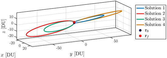
Figure 2. Transfer ellipses for Case 2 ($n_{\mathrm{rev}}=1$, $\Delta t=1500$ TU).

Case 3 ($n_{rev}={10}^5$, $\Delta t=1.5\times {10}^7$ TU). In spite of the very high number of revolutions, the ITA-method converges and finds all four solutions (cf. Table 8), with negligible degradation in accuracy. Final-position errors do not exceed $2\times {10}^{-5}$ DU. OL is able to detect only two out of four solutions, with greater accuracy, whereas ME identifies all four solutions (cf. Table 9), yet with lower accuracy compared to ITA (cf. Table 10). The four transfers ellipses are shown in Figure 3.

Table 8. Case 3 ($n_{rev}={10}^5$, $\Delta t=1.5\times {10}^7$ TU): orbit elements of transfer ellipses (ITA-method).

Solution	a [DU]	e	i [deg]	$\mathsf{\Omega }$ [deg]	$\mathit{\omega }$ [deg]	${\mathit{\theta }}_{\ast ,0}$ [deg]
1	8.291	0.9878	94.417	73.772	191.540	143.367
2	8.291	0.8946	94.417	73.772	12.660	322.247
3	8.291	0.8946	85.583	253.772	167.340	37.753
4	8.291	0.9878	85.583	253.772	348.460	216.633

Table 9. Case 3. Comparison of ITA with OL and ME: orbit elements displacements.

Method-Solution	$\Delta \mathit{a}$ [DU]	$\Delta \mathit{e}$	$\Delta \mathit{i}$ [deg]	$\Delta \mathsf{\Omega }$ [deg]	$\Delta \mathit{\omega }$ [deg]	$\Delta {\mathit{\theta }}_{\ast ,0}$ [deg]
OL-3	$1.2\times {10}^{-12}$	$1.6\times {10}^{-14}$	$1.4\times {10}^{-14}$	$2.8\times {10}^{-14}$	$8.5\times {10}^{-14}$	$1.0\times {10}^{-13}$
OL-4	$3.9\times {10}^{-12}$	$6.0\times {10}^{-15}$	$1.4\times {10}^{-14}$	$2.8\times {10}^{-14}$	$<{10}^{-16}$	$2.8\times {10}^{-14}$
ME-1	$1.5\times {10}^{-10}$	$2.3\times {10}^{-13}$	$<{10}^{-16}$	$<{10}^{-16}$	$1.4\times {10}^{-13}$	$1.4\times {10}^{-13}$
ME-2	$2.3\times {10}^{-9}$	$2.9\times {10}^{-11}$	$<{10}^{-16}$	$<{10}^{-16}$	$1.9\times {10}^{-11}$	$1.9\times {10}^{-11}$
ME-3	$1.5\times {10}^{-9}$	$1.9\times {10}^{-11}$	$1.4\times {10}^{-14}$	$2.8\times {10}^{-14}$	$1.2\times {10}^{-11}$	$1.2\times {10}^{-11}$
ME-4	$5.2\times {10}^{-10}$	$8.0\times {10}^{-13}$	$1.4\times {10}^{-14}$	$2.8\times {10}^{-14}$	$4.0\times {10}^{-13}$	$4.3\times {10}^{-13}$

Table 10. Case 3. Accuracy $\Delta r_f$ [DU] on the final position.

Method	Solution 1	Solution 2	Solution 3	Solution 4
ITA	$1.9\times {10}^{-5}$	$3.0\times {10}^{-6}$	$5.1\times {10}^{-6}$	$1.5\times {10}^{-5}$
OL	—	—	$3.8\times {10}^{-7}$	$5.2\times {10}^{-7}$
ME	$5.8\times {10}^{-4}$	$8.7\times {10}^{-3}$	$5.6\times {10}^{-3}$	$2.0\times {10}^{-3}$

Figure 3. Transfer ellipses for Case 3 ($n_{\mathrm{rev}}={10}^5$, $\Delta t=1.5\times {10}^7$ TU).

Case 4 ($n_{rev}={10}^6$, $\Delta t=1.5\times {10}^8$ TU). With an extremely high number of revolutions, the ITA-method still converges and finds all four solutions, with modest degradation in accuracy (cf. Table 11) in comparison with the preceding case. Final-position errors do not exceed $2\times {10}^{-4}$ DU. OL is able to detect only three out of four solutions, though with higher accuracy, whereas ME identifies all four transfer ellipses, yet with reduced accuracy compared to ITA (cf. Table 12 and Table 13). In particular, ME exhibits low accuracy for three out of four solutions (namely, 2, 3, and 4). The four transfers ellipses found with the ITA-method are indistinguishable from those depicted in Figure 3.

Table 11. Case 4 ($n_{rev}={10}^6$, $\Delta t=1.5\times {10}^8$ TU): orbit elements of transfer ellipses (ITA-method).

Solution	a [DU]	e	i [deg]	$\mathsf{\Omega }$ [deg]	$\mathit{\omega }$ [deg]	${\mathit{\theta }}_{\ast ,0}$ [deg]
1	8.291	0.9878	94.417	73.772	191.540	143.367
2	8.291	0.8946	94.417	73.772	12.660	322.247
3	8.291	0.8946	85.583	253.772	167.340	37.753
4	8.291	0.9878	85.583	253.772	348.460	216.633

Table 12. Case 4. Comparison of ITA with OL and ME: orbit elements displacements.

Method-Solution	$\Delta \mathit{a}$ [DU]	$\Delta \mathit{e}$	$\Delta \mathit{i}$ [deg]	$\Delta \mathsf{\Omega }$ [deg]	$\Delta \mathit{\omega }$ [deg]	$\Delta {\mathit{\theta }}_{\ast ,0}$ [deg]
OL-1	$2.0\times {10}^{-11}$	$3.1\times {10}^{-14}$	$<{10}^{-16}$	$1.4\times {10}^{-14}$	$5.7\times {10}^{-14}$	$<{10}^{-16}$
OL-2	$4.0\times {10}^{-12}$	$5.1\times {10}^{-14}$	$<{10}^{-16}$	$<{10}^{-16}$	$3.6\times {10}^{-15}$	$<{10}^{-16}$
OL-4	$9.4\times {10}^{-12}$	$1.5\times {10}^{-14}$	$1.4\times {10}^{-14}$	$2.8\times {10}^{-14}$	$<{10}^{-16}$	$2.8\times {10}^{-14}$
ME-1	$1.5\times {10}^{-9}$	$2.3\times {10}^{-12}$	$1.4\times {10}^{-14}$	$<{10}^{-16}$	$1.3\times {10}^{-12}$	$1.3\times {10}^{-12}$
ME-2	$3.7\times {10}^{-9}$	$4.7\times {10}^{-11}$	$<{10}^{-16}$	$<{10}^{-16}$	$3.1\times {10}^{-11}$	$3.1\times {10}^{-11}$
ME-3	$7.1\times {10}^{-9}$	$9.1\times {10}^{-11}$	$1.4\times {10}^{-14}$	$2.8\times {10}^{-14}$	$6.0\times {10}^{-11}$	$6.0\times {10}^{-11}$
ME-4	$2.8\times {10}^{-9}$	$4.3\times {10}^{-12}$	$1.4\times {10}^{-14}$	$2.8\times {10}^{-14}$	$2.3\times {10}^{-12}$	$2.3\times {10}^{-12}$

Table 13. Case 4. Accuracy $\Delta r_f$ [DU] on the final position.

Method	Solution 1	Solution 2	Solution 3	Solution 4
ITA	$7.5\times {10}^{-4}$	$1.5\times {10}^{-4}$	$4.1\times {10}^{-5}$	$3.6\times {10}^{-4}$
OL	$1.4\times {10}^{-5}$	$6.4\times {10}^{-7}$	—	$2.2\times {10}^{-6}$
ME	$5.5\times {10}^{-2}$	$1.4\times {10}^{-1}$	$2.8\times {10}^{-1}$	$1.1\times {10}^{-1}$

Case 5 ($n_{rev}={10}^4$, $\Delta t=1.5\times {10}^7$ TU). This scenario corresponds to a transfer angle equal to 179.97°, very close to the antipodal configuration. The ITA-method is able to detect all four solutions with great accuracy, never exceeding ${10}^{-11}$ DU (cf. Table 14). OL and ME are able to identify all solutions as well (cf. Table 15 and Table 16), with satisfactory—though much lower—accuracy (of order ${10}^{-8}$ DU and ${10}^{-6}$ DU, respectively).

Table 14. Case 5 ($n_{rev}=300$, $\Delta t={10}^4$ TU): orbit elements of transfer ellipses (ITA-method).

Solution	a [DU]	e	i [deg]	$\mathsf{\Omega }$ [deg]	$\mathit{\omega }$ [deg]	${\mathit{\theta }}_{\ast ,0}$ [deg]
1	3.040	0.4495	98.049	45.000	144.633	276.113
2	3.037	0.4486	98.049	45.000	336.842	83.904
3	3.040	0.4497	81.951	225.000	203.172	276.081
4	3.037	0.4484	81.951	225.000	35.382	83.872

Table 15. Case 5. Comparison of ITA with OL and ME: orbit elements displacements.

Method-Solution	$\Delta \mathit{a}$ [DU]	$\Delta \mathit{e}$	$\Delta \mathit{i}$ [deg]	$\Delta \mathsf{\Omega }$ [deg]	$\Delta \mathit{\omega }$ [deg]	$\Delta {\mathit{\theta }}_{\ast ,0}$ [deg]
OL-1	$3.1\times {10}^{-12}$	$2.1\times {10}^{-13}$	$8.0\times {10}^{-13}$	$1.4\times {10}^{-12}$	$1.0\times {10}^{-10}$	$1.0\times {10}^{-10}$
OL-2	$3.1\times {10}^{-12}$	$2.1\times {10}^{-13}$	$8.0\times {10}^{-13}$	$1.4\times {10}^{-12}$	$1.0\times {10}^{-10}$	$1.0\times {10}^{-10}$
OL-3	$3.2\times {10}^{-12}$	$2.2\times {10}^{-13}$	$8.0\times {10}^{-13}$	$1.5\times {10}^{-12}$	$1.0\times {10}^{-10}$	$1.0\times {10}^{-10}$
OL-4	$3.1\times {10}^{-12}$	$2.1\times {10}^{-13}$	$8.0\times {10}^{-13}$	$1.5\times {10}^{-12}$	$1.0\times {10}^{-10}$	$1.0\times {10}^{-10}$
ME-1	$7.5\times {10}^{-10}$	$6.0\times {10}^{-11}$	$1.6\times {10}^{-12}$	$2.3\times {10}^{-12}$	$2.3\times {10}^{-8}$	$2.3\times {10}^{-8}$
ME-2	$7.4\times {10}^{-10}$	$5.8\times {10}^{-11}$	$8.8\times {10}^{-13}$	$1.6\times {10}^{-12}$	$2.3\times {10}^{-8}$	$2.3\times {10}^{-8}$
ME-3	$7.6\times {10}^{-10}$	$6.0\times {10}^{-11}$	$4.9\times {10}^{-12}$	$8.8\times {10}^{-12}$	$2.4\times {10}^{-8}$	$2.4\times {10}^{-8}$
ME-4	$7.6\times {10}^{-10}$	$6.1\times {10}^{-11}$	$2.1\times {10}^{-13}$	$4.0\times {10}^{-13}$	$2.4\times {10}^{-8}$	$2.4\times {10}^{-8}$

Table 16. Case 5. Accuracy $\Delta r_f$ [DU] on the final position.

Method	Solution 1	Solution 2	Solution 3	Solution 4
ITA	$4.3\times {10}^{-12}$	$4.6\times {10}^{-12}$	$1.1\times {10}^{-11}$	$8.6\times {10}^{-13}$
OL	$1.1\times {10}^{-8}$	$1.1\times {10}^{-8}$	$1.1\times {10}^{-8}$	$1.0\times {10}^{-8}$
ME	$2.5\times {10}^{-6}$	$2.5\times {10}^{-6}$	$2.5\times {10}^{-6}$	$2.5\times {10}^{-6}$

From inspection of Table 3, Table 6, Table 9, Table 12 and Table 15, it is apparent that the orbit elements yielded by the three different methods are very close, even when the related accuracy is rather different (in particular, cf. Table 12 and Table 13). This can be explained by the high sensitivity of the results to the orbit semimajor axis, especially in the case of extremely large number of revolutions (e.g., in case 4). In particular, scenarios 3 and 4 also exhibit a typical property of solutions with an extremely high number of revolutions: direct and retrograde transfer ellipses tend to become indistinguishable in pairs as $n_{rev}$ increases. In fact, from inspection of Table 8 and Table 11 it is apparent that semimajor axis and eccentricity are identical (up to the third figure), for pairs (i) 1 and 4 and (ii) 2 and 3, while the angular momentum vectors of each pair are opposite. For this reason, in Figure 3, only two ellipses are clearly distinguishable. However, each of them corresponds to two distinct orbits, traveled in opposite directions. With regard to case 5, the near-antipodal boundary conditions lead to finding 4 ellipses that are again nearly indistinguishable in pairs. This is apparent in Figure 4 and from inspection of Table 14, and it is consistent with the degeneracy that occurs with antipodal terminal positions (cf. Section 3.1).

Figure 4. Transfer ellipses for Case 5 ($n_{\mathrm{rev}}=300$, $\Delta t={10}^4$ TU).

In summary, the five test cases investigated in this section show that

• ITA is able to identify all four ellipses in all cases, as well as ME; OL yields an incomplete set of solutions in four out of five cases;
• ITA yields solutions with very satisfactory accuracy across all scenarios, and
  • outperforms ME in both ultra-revolution regimes (i.e., cases 3 and 4) and the near-antipodal configuration (scenario 5), while ME exhibits superior accuracy in cases 1 and 2;
  • outperforms OL in scenarios 1 and 5, while accuracy of OL is superior in the incomplete set of solutions found in cases 3 and 4 (ultra-revolution regimes).

As a final remark, for the ITA-method the capability of detecting all solutions is clearly related to the effectiveness of the search process for all the solutions of Equation (15) over the entire interval of admissible values for the true anomaly, identified by Equations (26) and (33).

4.3. Earth–Mars Interplanetary Transfer

The ITA-method can also be applied to investigating feasibility and performance of interplanetary transfers. As an illustrative example, this subsection considers Earth-Mars mission opportunities, i.e., the feasible interplanetary transfer paths that drive a spacecraft from Earth to Mars, leveraging the patched conics approximation [44], a well-established technique widely used for preliminary interplanetary mission analysis. The positions of the two planets are obtained from planetary ephemeris, using the interpolation provided by Curtis [44]. Only the interplanetary transfer arc is investigated, which means that planetocentric trajectories (within the spheres of influence of either Earth or Mars) are not considered, because the latter arcs are traveled in very short time intervals, compared to the interplanetary transfer trajectory.

Four different study cases are introduced: (i) direct transfer ($n_{rev}=0$), (ii) single-revolution transfer ($n_{rev}=1$), (iii) two-revolution transfer ($n_{rev}=2$), and (iv) three-revolution transfer ($n_{rev}=3$). For each case, a specific range for the time of flight ($\Delta t$) is considered, namely,

• $n_{rev}=0$: $\Delta t\in [200,600]$ days;
• $n_{rev}=1$: $\Delta t\in [600,1200]$ days;
• $n_{rev}=2$: $\Delta t\in [1000,1900]$ days;
• $n_{rev}=3$: $\Delta t\in [1600,2500]$ days.

while the departure date is sought over a 6-year interval, i.e., $t_0\in [2026,2032]$.

Figure 5, Figure 6, Figure 7 and Figure 8 depict the porkchop plots, with departure time and time of flight along the x-axis and y-axis, respectively. These represent the contour plots of the overall velocity change $\Delta v_{tot}$ needed to travel the interplanetary trajectory, with $\Delta v_{tot}=\Delta v_1+\Delta v_2$, where (a) $\Delta v_1$ properly represents the spacecraft velocity relative to the Earth while leaving its sphere of influence, whereas (b) $\Delta v_2$ is the velocity relative to Mars while entering its sphere of influence. Values for $\Delta v_{tot}$ greater than 15 km/s are discarded. Inspection of Figure 5, Figure 6 and Figure 7 allows finding the optimal transfer option, associated with the minimum $\Delta v_{tot}$ in each scenario, together with the respective departure date, time of flight, and error at Mars encounter. It is worth remarking that in the context of the patched conic approximation [44], the spacecraft is expected to target the sphere of influence of the arrival planet. However, due to the typical (very large) distances traveled in the interplanetary transfer arc in comparison with the radius of the sphere of influence, the latter is identified with the instantaneous position of the center of Mars. Obviously, after entering this sphere, the space probe is subject to the dominating attraction of the planet. Nevertheless, in Table 17, the values of $\Delta r_f$ are reported for illustrative purposes, and turn out to be modest, which again testifies to the high accuracy of the solution method.

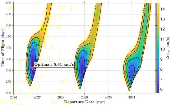
Figure 5. Earth –Mars transfer: porkchop plot ($n_{rev}=0$).

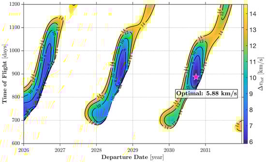
Figure 6. Earth–Mars transfer: porkchop plot ($n_{rev}=1$).

Figure 7. Earth–Mars transfer: porkchop plot ($n_{rev}=2$).

Figure 8. Earth–Mars transfer: porkchop plot ($n_{rev}=3$).

Table 17. Optimal Earth–Mars interplanetary transfer.

${\mathit{n}}_{\mathit{rev}}$	${\mathit{t}}_0$	$\Delta \mathit{t}$ [days]	$\Delta {\mathit{v}}_{\mathit{tot}}$ [km/s]	$\Delta {\mathit{r}}_{\mathit{f}}$ [km]
0	10/31/2026	311	5.608	$6.8\times {10}^{-6}$
1	09/28/2030	887	5.882	$5.6\times {10}^{-6}$
2	11/09/2027	1332	5.694	$1.4\times {10}^{-6}$
3	10/22/2031	1911	5.611	$2.2\times {10}^{-6}$

The preceding preliminary mission analysis represents a rather standard use of a Lambert solver, and definitely points out the usefulness, versatility, and effectiveness of the ITA-method in a scenario of practical interest, in the context of interplanetary trajectories.

5. Concluding Remarks

Multi-revolution Lambert solvers are intended to find the elliptic transfer orbits that are traveled multiple times and connect two prescribed positions in specified time. This study proposes and tests a new, effective multi-revolution Lambert solver, based on elementary calculus and employing the initial true anomaly along the transfer ellipse as the unknown variable. The related search interval is analyzed and identified through closed-form expressions for upper and lower bounds. Moreover, some remarkable special cases are also analyzed. The fundamental solving equation is written in explicit form, with the initial true anomaly as the only unknown. A simple numerical algorithm, based on the regula falsi, is employed, to detect all the Lambert solutions. First, the entire search interval is split in subarcs. Second, in each subarc the regula falsi is applied. Lastly, if all solutions are not detected, then the number of subarcs is increased and the process is repeated, until all transfer paths are found. The entire numerical solution process is described in detail in Section 3.5. Because orbit elements and well-established relations of Keplerian motion are utilized, the ITA-method, proposed in this research, is rather simple to understand and straightforward to implement. In fact, elementary calculus and intuitive quantities, with straighforward geometrical interpretation, are employed, unlike alternative techniques that require introducing much less intuitive variables or even contour integrals in the complex domain. The new multi-revolution solver proposed in this study is successfully tested in several challenging scenarios, corresponding to some pathological cases reported in the recent scientific literature. Comparison with alternative, up-to-date techniques regard accuracy and capability of finding all four solutions. The ITA-solver turns out to find all the feasible transfer ellipses, in all cases, with very satisfactory accuracy in terms of final position error. More specifically, the ITA-solver outperforms the Oldenhuis implementation in terms of robustness, i.e., capability of finding all solutions, and is highly competitive with the recently-introduced approach by McElreath et al. in terms of accuracy on the final position, if the number of revolutions is large. Definitely, the numerical results show that it can represent a valuable option to find all Lambert solutions, even in challenging scenarios that include a huge number of revolutions or near-antipodal terminal positions. As a further illustrative example, the ITA-method is successfully applied to determining the mission opportunities and the related minimum-fuel solutions for Earth–Mars transfers, in the context of a typical preliminary interplanetary mission analysis.

It is worth remarking that the multi-revolution solver proposed and designed in this research, as well as the counterparts considered for comparison, assume Keplerian motion, under the influence of a single attracting body. However, in some specific mission scenarios, orbit perturbations play a role (e.g., harmonics of the gravitational potential and third body gravitational pull), while the effects of general relativity may become nonnegligible, in the presence of a very massive attracting body and huge number of revolutions. This circumstance implies the need of numerically adjusting Lambert solutions. Nevertheless, the latter paths, Keplerian in nature, can represent suitable first-attempt solutions, extremely useful to get numerical results adherent to the perturbed (non-Keplerian) dynamical environment of interest.

References

- De Lagrange, J.L. Mecanique Analytique; Académie des Sciences: Paris, France, 1788; Volume 2. [Google Scholar]
- Gauss, C.F. Theory of the Motion of the Heavenly Bodies Moving About the Sun in Conic Sections: A Translation of Carl Frdr. Gauss “Theoria Motus”; Little, Brown and Company: New York, NY, USA, 1857. [Google Scholar]
- de la Torre Sangrà, D.; Fantino, E. Review of Lambert’s problem. ISSFD 2015, 2015, 25. [Google Scholar]
- MacLellan, S.J. Orbital Rendezvous using an Augmented Lambert Guidance Scheme. Ph.D. Thesis, Massachusetts Institute of Technology, Cambridge, MA, USA, 2005. [Google Scholar]
- Thorne, J.D.; Bain, R.D. Series reversion/inversion of Lambert’s time function. J. Astronaut. Sci. 1995, 42, 277–287. [Google Scholar]
- Thorne, J.D. Convergence behavior of series solutions of the Lambert problem. J. Guid. Control. Dyn. 2015, 38, 1821–1826. [Google Scholar] [CrossRef]
- Prussing, J.E. A class of optimal two-impulse rendezvous using multiple-revolution Lambert solutions. J. Astronaut. Sci. 2000, 48, 131–148. [Google Scholar] [CrossRef]
- Chen, T.; Van Kampen, E.; Yu, H.; Chu, Q. Optimization of time-open constrained Lambert rendezvous using interval analysis. J. Guid. Control. Dyn. 2013, 36, 175–184. [Google Scholar] [CrossRef]
- Bate Roger, R.; Mueller Donald, D.; Jerry, E. Fundamentals of Astrodynamics; Dover: Mineola, NY, USA, 1971. [Google Scholar]
- Wailliez, S.E. On Lambert’s problem and the elliptic time of flight equation: A simple semi-analytical inversion method. Adv. Space Res. 2014, 53, 890–898. [Google Scholar] [CrossRef]
- Herrick, S.; Liu, A. Two body orbit determination from two positions and time of flight. Append. A Aeronutronic 1959, 365. [Google Scholar]
- Boltz, F.W. Second-order p-iterative solution of the Lambert/Gauss problem. J. Astronaut. Sci. 1984, 32, 475–485. [Google Scholar]
- Avanzini, G. A simple Lambert algorithm. J. Guid. Control Dyn. 2008, 31, 1587–1594. [Google Scholar] [CrossRef]
- He, Q.; Li, J.; Han, C. Multiple-revolution solutions of the transverse-eccentricity-based lambert problem. J. Guid. Control Dyn. 2010, 33, 265–269. [Google Scholar] [CrossRef]
- Zhang, G.; Mortari, D.; Zhou, D. Constrained multiple-revolution Lambert’s problem. J. Guid. Control Dyn. 2010, 33, 1779–1786. [Google Scholar] [CrossRef]
- Zhang, G.; Zhou, D.; Mortari, D. Optimal two-impulse rendezvous using constrained multiple-revolution Lambert solutions. Celest. Mech. Dyn. Astron. 2011, 110, 305–317. [Google Scholar] [CrossRef]
- Wen, C.; Zhao, Y.; Shi, P. Derivative analysis and algorithm modification of transverse-eccentricity-based Lambert problem. J. Guid. Control Dyn. 2014, 37, 1195–1201. [Google Scholar] [CrossRef]
- Simó, C. Solución del problema de Lambert mediante regularización. Collect. Math. 1973, 24, 231–248. [Google Scholar]
- Kriz, J. A uniform solution of the Lambert problem. Celest. Mech. 1976, 14, 509–513. [Google Scholar] [CrossRef]
- Lancaster, E.R. Solution for Lambert Problem for Short Arcs; Technical Report; NASA Goddard Space Flight Center: Greenbelt, MD, USA, 1969.
- Gooding, R.H. On the Solution of Lambert’s Orbital Boundary-Value Problem; Technical Report; Royal Aerospace Establishment: Farnborough, UK, 1988. [Google Scholar]
- Gooding, R.H. A procedure for the solution of Lambert’s orbital boundary-value problem. Celest. Mech. Dyn. Astron. 1990, 48, 145–165. [Google Scholar] [CrossRef]
- Izzo, D. Revisiting Lambert’s problem. Celest. Mech. Dyn. Astron. 2015, 121, 1–15. [Google Scholar] [CrossRef]
- Vallado, D.A. Fundamentals of Astrodynamics and Applications; McGraw-Hill Companies: Columbus, OH, USA, 1997. [Google Scholar]
- Luo, Q.; Meng, Z.; Han, C. Solution algorithm of a quasi-Lambert’s problem with fixed flight-direction angle constraint. Celest. Mech. Dyn. Astron. 2011, 109, 409–427. [Google Scholar] [CrossRef]
- Thompson, B.F. Enhancing lambert targeting methods to accommodate 180-degree orbital transfers. J. Guid. Control Dyn. 2011, 34, 1925–1929. [Google Scholar] [CrossRef]
- Arora, N.; Russell, R.P. A fast and robust multiple revolution Lambert algorithm using a cosine transformation. Adv. Astronaut. Sci. 2014, 150, 411–430. [Google Scholar]
- Battin, R.H.; Vaughan, R.M. An elegant Lambert algorithm. J. Guid. Control Dyn. 1984, 7, 662–670. [Google Scholar] [CrossRef]
- Loechler, L.A. An elegant Lambert algorithm for multiple revolution orbits. PhD Thesis, Massachusetts Institute of Technology, Cambridge, MA, USA, 1988. [Google Scholar]
- Shen, H.; Tsiotras, P. Using Battin’s Method To Obtain Multiple-Revolution Lambert’ S Solutions. Adv. Astronaut. Sci. 2004, 116, 1–18. [Google Scholar]
- Battin, R.H. Lambert’s problem revisited. Aiaa J. 1977, 15, 707–713. [Google Scholar] [CrossRef]
- Battin, R.H. An Introduction to the Mathematics and Methods of Astrodynamics; AIAA: Reston, VA, USA, 1999. [Google Scholar]
- Jezewski, D.J. K/S two-point-boundary-value problems. Celest. Mech. 1976, 14, 105–111. [Google Scholar] [CrossRef]
- Lancaster, E.R.; Blanchard, R.C. A Unified form of Lambert’s Theorem; Technical Report, NASA TN D-5368; NASA: Greenbelt, MD, USA, 1969.
- Arora, N.; Russell, R.P.; Strange, N.; Ottesen, D. Partial derivatives of the solution to the Lambert boundary value problem. J. Guid. Control. Dyn. 2015, 38, 1563–1572. [Google Scholar] [CrossRef]
- Der, G.J. The Superior Lambert Algorithm; AMOS: Maui, HI, USA, 2011. [Google Scholar]
- Mahajan, B.; Vadali, S.R. Two-body orbital boundary value problems in regularized coordinates. J. Astronaut. Sci. 2020, 67, 387–426. [Google Scholar] [CrossRef]
- Ochoa, S.I.; Prussing, J.E. Multiple revolution solutions to Lambert’s problem. Adv. Astronaut. Sci. 1992, 79, 1205–1216. [Google Scholar]
- Russell, R.P. On the solution to every Lambert problem. Celest. Mech. Dyn. Astron. 2019, 131, 50. [Google Scholar] [CrossRef]
- Russell, R.P. Complete Lambert solver including second-order sensitivities. J. Guid. Control Dyn. 2022, 45, 196–212. [Google Scholar] [CrossRef]
- Negrete, A.; Abdelkhalik, O.O. Exact solution to lambert’s problem using contour integrals. J. Guid. Control Dyn. 2025, 48, 771–780. [Google Scholar] [CrossRef]
- McElreath, J.; Down, I.M.; Majji, M. A universal approach for solving the multi-revolution Lambert’s problem. Celest. Mech. Dyn. Astron. 2025, 137, 22. [Google Scholar] [CrossRef]
- Oldenhuis, R. Robust Solver for Lambert’s Orbital-Boundary Value Problem. Available online: https://github.com/rodyo/FEX-Lambert/releases/tag/v1.4 (accessed on 19 October 2025).
- Curtis, H.D. Orbital Mechanics for Engineering Students; Butterworth-Heinemann: Oxford, UK, 2019. [Google Scholar]
- Prussing, J.E.; Conway, B.A. Orbital Mechanics; Oxford University Press: Oxford, UK, 1993. [Google Scholar]
- McElreath, J. A Universal Multi-Revolution Lambert Solver. Available online: https://it.mathworks.com/matlabcentral/fileexchange/181322-a-universal-multi-revolution-lambert-solver (accessed on 19 October 2025).
Disclaimer/Publisher’s Note: The statements, opinions and data contained in all publications are solely those of the individual author(s) and contributor(s) and not of MDPI and/or the editor(s). MDPI and/or the editor(s) disclaim responsibility for any injury to people or property resulting from any ideas, methods, instructions or products referred to in the content. |
© 2026 by the authors. Licensee MDPI, Basel, Switzerland. This article is an open access article distributed under the terms and conditions of the Creative Commons Attribution (CC BY) license.