Abstract
In this study, we develop and analyze an extended SEIR-type compartmental model that incorporates vaccination and treatment to describe the dynamics of acute respiratory infection transmission. The model subdivides the infectious population into several symptomatic stages and an asymptomatic class, which allows the evaluation of control strategies across different levels of infection severity. The basic reproduction number is analytically derived, and its sensitivity to vaccination and treatment rates is examined to assess the impact of public health interventions on epidemic control. Numerical simulations demonstrate that the joint implementation of vaccination and treatment can markedly reduce disease prevalence and lead to infection elimination when . The results emphasize the critical role of parameter interactions in determining disease persistence and show that combining both interventions produces stronger epidemiological effects than either one alone. Machine learning techniques, specifically Support Vector Machines (SVMs), are employed to classify epidemiological outcomes and support parameter estimation. The biological markers evaluated were not effective discriminants of infection status, underscoring the importance of integrating mechanistic modeling with data-driven approaches. This combined framework enhances the understanding of epidemic dynamics and improves the predictive capacity for decision-making in public health.
1. Introduction
Mathematical epidemiology has emerged as a central discipline for understanding the spread, control, and prediction of infectious diseases. By integrating concepts from biology, medicine, and mathematics, it enables the formulation and analysis of models that provide both qualitative insights and quantitative guidance for public health. The foundational work of Kermack and McKendrick in 1927 [1] introduced the classical SIR (Susceptible–Infected–Removed) model, describing the spread of infection in a homogeneous, closed population with permanent immunity and no vital dynamics. Their seminal analysis highlighted the role of a threshold parameter, defined as the ratio of transmission to recovery rates, which determines whether an epidemic outbreak occurs, thereby laying the conceptual foundation of threshold dynamics in epidemiology.
Over the decades, compartmental models have been extensively refined to incorporate greater biological realism and intervention strategies, notably vaccination and treatment. SEIR-type models, which explicitly include a latent or exposed class, have become a standard framework for analyzing epidemic dynamics and evaluating control measures [2,3]. For instance, Ledder [4] developed a SEIRV model to study how vaccination coverage modifies the basic reproduction number and epidemic peaks, demonstrating that partial immunization can substantially reduce outbreak size even when herd immunity is not achieved. Antonelli et al. [5] extended this approach through a hybrid SEIRDV framework for COVID-19 in Italy, showing how vaccination campaigns alter epidemic trajectories over time. Hou and Bidkhori [6] incorporated multi-feature population heterogeneity to optimize vaccine allocation at subregional levels, emphasizing the importance of prioritization strategies. Similarly, Li et al. [7] and Kiselev et al. [8] studied the synergistic effects of treatment and preventive strategies, highlighting how antiviral therapies and vaccination can jointly reduce transmission and accelerate recovery.
Recent advances in mathematical epidemiology have highlighted the importance of incorporating vaccination, treatment, and immunity loss into epidemic models to describe the persistence and recurrence of infectious diseases. For example, Lacy et al. (2023) [9] developed a compartmental model that integrates vaccination effects and behavioral dynamics to evaluate the impact of immunization campaigns on COVID-19 transmission in St. Louis. Their results emphasize that even high vaccination coverage may not completely suppress disease resurgence if contact patterns remain unchanged, reflecting the intricate interplay between immunity and human behavior. Similarly, Han et al. (2022) [10] proposed a VSEIR framework that explicitly includes vaccination efficacy and immune decline, demonstrating how reduced vaccine protection over time can lead to oscillatory or endemic dynamics. These findings underscore the need to incorporate waning immunity in realistic models of long-term disease persistence. Extending this perspective, Pathak and Kota (2025) [11] introduced a time-delayed epidemic model combining vaccination and treatment interventions, accounting for delays in vaccine preparation, administration, and the progression from infection to recovery. Their study analytically examined both local and global stability conditions through the basic reproduction number and Lyapunov functionals, providing insight into the complex temporal feedback mechanisms that influence disease control. Altogether, these recent models illustrate that integrating vaccination, treatment, and temporal delays into mathematical formulations can capture richer epidemic behaviors, particularly in systems where viral load dynamics or internal infection states drive transitions between infection, recovery, and reinfection.
Complementary works have examined nonlinear saturation, age-structured immunity, and combined pharmaceutical and non-pharmaceutical interventions [12,13,14], collectively forming a rich literature on SEIR-based epidemic control.
In parallel, multiscale modeling has provided a powerful lens to bridge in-host pathogen dynamics and population-level transmission. Studies of influenza and COVID-19 have shown that immune responses, co-infections, and within-host progression critically shape disease kinetics and transmission [15,16,17]. These approaches also enable the derivation of macroscopic epidemic models from individual-based or kinetic perspectives [18,19,20,21], incorporating contact heterogeneity and behavioral variability. For instance, Della Marca et al. (2023) derived an SIR model from a microscopic formulation where each agent possesses an internal infection state modulating transmissibility [18], while Dimarco et al. (2021) demonstrated how epidemic waves emerge from agent interactions with heterogeneous contact rates [19]. Dimarco, Toscani, and collaborators further investigated optimal control in socially heterogeneous populations [20], and Bondesan et al. (2025) proposed a multiscale framework linking individual-level disease progression with observable epidemic indicators [22]. These developments justify measurable differences in transmission across symptomatic stages and support the stratified compartmental structures adopted here.
While multiscale approaches provide valuable theoretical insight into the interplay between biological and social timescales [15,16,17,18,19,20,21,22], their direct application to epidemic control is often secondary to compartmental interventions such as vaccination, treatment, and behavioral modulation. Nevertheless, evidence from immunological studies and host–pathogen interactions supports the stratification of infectious stages and the inclusion of asymptomatic carriers in population-level models [23,24,25,26,27]. This motivates the adoption of multiple symptomatic stages and an asymptomatic class in the present work, ensuring that transmission heterogeneity and stage-specific intervention effects are explicitly captured.
Concurrently, machine learning (ML) has become increasingly important in epidemic analysis, particularly when coupled with mechanistic models. ML algorithms enhance parameter estimation, outbreak forecasting, and classification of epidemic regimes, complementing the predictive power of compartmental frameworks [28,29,30]. Among ML approaches, Support Vector Machines (SVMs) stand out for their robustness in high-dimensional, limited-sample contexts [31,32,33,34]. SVMs identify optimal separating boundaries between outcome classes using support vectors, enabling nonlinear classification of clinical or epidemiological data. In infectious disease research, SVMs have been successfully employed for early risk stratification, epidemic phase classification, and identifying dominant transmission drivers [35,36].
The present study introduces a hybrid framework that couples a mechanistic SEIR-type model with data-driven SVM analysis. The model subdivides the infectious population into three symptomatic stages and an asymptomatic class, incorporating vaccination and treatment processes. This structure allows a detailed assessment of intervention effects at different infection stages and supports analytical derivation of the basic reproduction number and its sensitivity to control parameters. Simultaneously, SVM is applied to classify epidemic outcomes based on simulated and observed data, enhancing interpretability and offering a practical tool for decision support in epidemic response. The novelty of this work lies in integrating mechanistic and data-driven perspectives within a unified analytical framework that captures both theoretical and empirical dimensions of epidemic dynamics. This approach bridges mathematical epidemiology with computational intelligence, enabling more accurate prediction and adaptive control of infectious diseases.
Finally, in the Peruvian context, acute respiratory infections (ARIs) remain one of the leading causes of morbidity and mortality in children and older adults in Peru [37]. ARIs affect the upper and lower respiratory tract, are caused by viruses and bacteria, and typically last fewer than 15 days [38]. Common diseases include colds, influenza, bronchitis, pneumonia, and COVID-19, with etiological agents such as AH1N1, SARS-CoV-2, and Haemophilus influenzae. Clinically, ARIs present across a severity spectrum ranging from asymptomatic to critical infection. Given this national context, the present work develops a mathematical model for acute respiratory diseases and analyzes the effects of pharmacological treatment and vaccination in a population stratified according to disease severity.
2. Materials and Methods
2.1. Compartmental Model
The present model is characterized by the presence of four infected compartments according to the presence or absence of symptoms. The epidemiological states were asymptomatic (A, i.e., without clinical symptoms), infected with mild symptoms (), infected with moderate symptoms (), and infected with severe or severe symptoms (). The existence of a population of latent individuals (L), who are infected but do not transmit the disease, is considered. Once the incubation or latency time () has ended, we have complementary probabilities and for developing a disease with mild, moderate, severe, or no symptoms, respectively. On the other hand, the three types of symptomatic and asymptomatic infectious individuals can spread the disease with different intensity. Transition rate () also reflect symptom worsening. Infected populations recover their health with a recovery rate . With respect to those removed, these are divided into recovered (R) and dead by the disease (M) subpopulations. Moreover, asymptomatic individuals recover and do not die of the disease. The model incorporates life dynamics (: constant growth rate; : death rate) and assumes that there is no loss of immunity (total immunity), considering a dynamic of 4 months. In addition, exogenous factors, such as vaccination and symptomatological treatment (pharmacological, for example) are incorporated and affect the dynamics of the system. In the same context, immunization is performed with a vaccination rate () and at the same time a symptomatic infected person under treatment can reduce its severity (this effect is captured by the reversion rate , which are the inverse of the number of days needed for symptoms to decrease in severity owing to the effect of the treatment). Finally, we considered three different transmission rates per each symptomatic population ( for mildly, for moderately, and for severely infected populations), based on the assumption that moderately and severely infected have less effective propagation into the population; we also assumed that asymptomatic individuals can transmit the disease with less intensity than the mildly infected, which is represented by an attenuation rate .
All rates are constant because they are considered average values within the dynamic system. In addition, the recovery rates were similar for all the infected compartments. However, different mortality rates () were assumed for each compartment with symptomatic infection. In addition, for the total population at any instant of time t it is satisfied that: , where is the susceptible population. The flowchart of the model is shown in Figure 1:
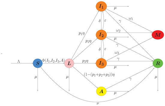
Figure 1.
Compartmental model.
Based on the above hypotheses and the dynamics described by the compartmental model, the dynamic system is formalized as follows.
We uncouple the system from the disease dead population (because its dynamics is determined by the compartments of symptomatic infected individuals) and replace the incidence given by in the system (1), with the infection rates , , and , by which we obtain a reduced system shown in the Appendix A.1.
2.2. Support Vector Machines (SVMs)
Support Vector Machines (SVMs) are supervised learning algorithms widely used for classification tasks in biomedical and epidemiological research [31,32]. The basic idea is to find an optimal separating hyperplane that maximizes the margin between two classes of data in a feature space. Given a set of training data with input vectors and class labels , the SVM constructs a decision function of the form
where is a kernel function, are nonnegative Lagrange multipliers, and b is the bias term. Only a subset of the training data contributes to the decision function; these are called support vectors, and they lie closest to the decision boundary. The optimization problem solved by SVM can be written as
where w is the normal vector to the separating hyperplane, are slack variables allowing some misclassification, is a regularization parameter controlling the trade-off between margin maximization and classification error, and is a nonlinear mapping of the data induced by the kernel function. In our case we used the radial basis function (RBF) kernel,
which allows nonlinear decision boundaries suitable for complex biomedical data [34].
An advantage of SVMs is their robustness in high-dimensional settings with relatively small sample sizes, making them particularly attractive for clinical biomarker analysis. In this work, we applied SVMs to classify patients into moderate or severe COVID-19 cases based on immunological markers (CD, IL-6, and TRPV-1). This approach is consistent with prior applications of SVMs in medical diagnostics, where they have been successfully used for tasks ranging from cancer detection to infectious disease classification [32,33].
2.3. Clinical Data
To exemplify the use of the proposed model, the following workflow was followed: First, patients were classified according to the severity of their symptoms using support vector machines (SVMs), and the flow of cases was recorded over a period of approximately four months (Supplementary Material S1). Second, the accumulated symptomatic case data (Supplementary Material S2) were used to estimate the parameters of the mathematical model (considering that there was no treatment or vaccination). Finally, we simulated the effect of treatment and vaccination on the development of infection using the estimated parameters on a population of susceptible individuals taken ad hoc.
To develop a classification model using SVM, a database of patients with COVID-19 provided by the Molecular Biology Unit of the Guillermo Almenara Irigoyen National Hospital (HNGAI) was used with respect to the privacy and confidentiality of the data in accordance with Law 29733 on Personal Data Protection (https://www.gob.pe/institucion/congreso-de-la-republica/normas-legales/243470-29733, accessed on 12 June 2025) and the principles of the Declaration of Helsinki (https://www.wma.net/es/policies-post/declaracion-de-helsinki-de-la-amm-principios-eticos-para-las-investigaciones-medicas-en-seres-humanos/, accessed on 12 June 2025). Patients clinically classified according to the technical document “Prevention and care of people affected by COVID-19 in Peru” [39] of the Peruvian Ministry of Health (https://www.gob.pe/institucion/minsa/normas-legales/465962-139-2020-minsa, accessed on 12 June 2025) corresponded to the period 01/07/2021 to 04/23/2021. However, due to the small sample size for mild cases (five cases), only moderate and severe cases were analyzed (Supplementary Material S1).
2.4. Integration of Epidemiological Modeling and SVM Classification
Our analysis explicitly emphasizes the complementarity between the epidemic modeling and SVM classification frameworks. The compartmental model captures the temporal dynamics of infection across symptomatic stages, whereas the SVM provides a data-driven stratification of patients based on clinical biomarkers. This correspondence allows for mapping the SVM-derived classes (moderate and severe) to the epidemic compartments and , respectively, linking individual-level heterogeneity with population-level transmission.
The outputs of the compartmental model, such as incidence trajectories and the estimated basic reproduction number , contextualize the observed patient distributions and the epidemiological stage in which classification occurs. Conversely, the SVM feature contributions—particularly those of IL-6, TRPV-1, and CD—inform the biological interpretation of transitions between disease stages in the model.
This integrative approach ensures conceptual coherence between the mechanistic and data-driven components: the epidemic model explains how infection propagates through a population, while the SVM clarifies how host-level immunological variation manifests across clinical categories. Together, they provide a unified multiscale perspective on the epidemic process.
3. Results
3.1. Derivation of the Basic Reproduction Number
In the study of mathematical models in epidemiology, a critical epidemiological parameter has been determined, which is the basic reproduction number () defined as the average number of secondary infections that an infected individual can carry out when in contact with a population susceptible to contracting the disease [40], the calculation of this parameter allows us to determine deterministically whether an epidemic is endemic () or not ().
This parameter was calculated using the next generation matrix method [41,42] and we found the following (calculation details can be reviewed in Appendix A.2):
where
3.2. Analytical Solvability
Several classical SIR-type epidemic models admit exact or semi-analytic solutions under restrictive structural assumptions. For instance, Harko et al. [43] and Schlickeiser and Kröger [44,45] derived closed-form solutions for the standard SIR formulation and certain extensions with time-dependent infection or recovery rates. These analytical constructions rely on the low dimensionality of the SIR system and on its reducibility to a single separable differential equation or to integrable forms via conserved quantities. By contrast, the model developed in the present study includes a latent class (L), three symptomatic infectious classes (), an asymptomatic class (A), vaccination, and pharmacological treatment terms that allow both progression and reversion of symptoms. The infection process couples multiple infectious subpopulations through the nonlinear incidence term , which prevents any analytical decoupling of the system into one or two scalar equations. In addition, class-specific recovery and mortality rates further break the separability conditions required for analytic integrability. For these reasons, the current model cannot be solved in closed form following the methods used for classical SIR-type systems. Consequently, we focused on analytical–numerical methods, including the derivation of , sensitivity and numerical simulations. Future work could, however, investigate local stability, conduct a bifurcation analysis, and approximate analytical reductions under suitable simplifying assumptions such as aggregation of infectious stages or time-scale separation.
3.3. Theoretical Results
3.3.1. Simulations for Disease-Free and Endemic Scenarios
To illustrate the disease-free and endemic scenarios, the initial conditions vector the populations considered were: (Figure 2 and Figure 3). The ranges of parameter values listed in Table 1 are based on COVID-19 and the specific parameter values are shown in each figure.
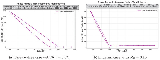
Figure 2.
Phase portraits for infected vs. non-infected populations in two possible scenarios.
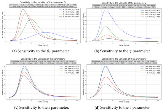
Figure 3.
Sensitivity to some parameters for the moderately infected curve. Initial conditions , and the rest of initial populations equal to zero.

Table 1.
Parameters of the SLIIIARM model.
The simulations whereas the computational sensitivity analysis were performed using Scipy 1.16.3, Numpy 1.26.4 and Matplotlib 3.3.4 packages and they were implemented in Python version 3.8. Figure 2a,b show the disease-free and endemic cases, respectively, where the infected populations tended to disappear or remain constant, which is corroborated by the simulated phase diagrams for 720 days in both cases. The tornado plot was developed using a Shiny application built with R language.
3.3.2. Computational Sensitivity
For the sensitivity analysis of the numerical solutions, the effect of varying the parameters on the moderately infected population was analyzed because it represents a critical stage between a better diagnosis (mild symptoms) or a worse stage (severe symptoms). We chose the main transmission () and the recovery rates (). We observe that as increases (Figure 3a), there is a more pronounced peak in the number of infected, and in a shorter time since the beginning of the epidemic, it also shifts us from disease-free () to endemic equilibrium (). In contrast, an increase in (Figure 3b) reduces the infected peak and slightly dilates their onset over time, the net effect being that it allows us to transition to a disease-free equilibrium. By improving the efficiency of treatment (increasing ), that is, by decreasing the time in which symptoms reverse and increasing the vaccination rate, moderate cases decreased (Figure 3c,d), but only allows us to get the disease-free equilibrium, indicating that this is a relevant factors in disease control.
3.3.3. Sensitivity Analysis of the Basic Reproductive Number
For the study of the sensitivity of , the partial rank correlation coefficients (PRCC) were used with Latin hypercube sampling (LHS) getting a sample of 5000 input parameters, where a normal distribution was assumed with a mean of 0.5, and a standard deviation of 0.2 for ; in the case of , the selected mean was 0.16975 and the standard deviation was 0.14275; for , the mean and standard deviation were 0.4 and 0.3, respectively; while for the rest of the parameters, a uniform distribution (see Appendix C) was used with the ranges given in Table 1 (Figure 4a). The results of this analysis show a negative correlation for (PRCC index absolute value: 0.41335) and , , and (PRCC index absolute value: 0.18551, 0.18079 and 0.11997, respectively), as well as a positive correlation for (PRCC index absolute value: 0.44715) and (PRCC index absolute value: 0.26998).
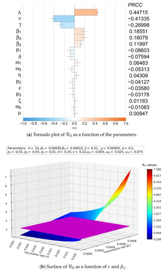
Figure 4.
Sensitivity of with respect to the parameters.
In addition, a decision surface of as a function of and was constructed, together with the plane (Figure 4b, plane in purple), to exemplify the analysis of the joint effect of two parameters with antagonistic effects on . There is a wide control region (blue shades) where we can combine vaccination strategies and trying to control the transmission rate (for example, using pharmaceutical interventions to diminish cough and sneezing, or isolating healthy people) to avoid endemic disease and lead us to the disease-free equilibrium point.
3.4. Study Case in a Peruvian Hospital
3.4.1. Classification Model Using Support Vector Machine
SARS-CoV-2 infection affects the neuroimmune system, causing microglial activation, cytokine storm, and adecrease in CD4 T cells (CD4+), resulting in an increase in the production of proinflammatory cytokines such as interleukin 6 (IL-6) and an increase in the expression of transient receptor potential vanilloid 1 (TRPV-1). TRPV-1 is expressed in neuronal cells, immune cells and respiratory sensory fibers, and its expression is increased in infections such as respiratory syncytial virus infections. An increase in TRPV-1 expression also increased IL-6 production. The activation of the neuroimmune pathway involving TRPV-1 expression and IL-6 production forms a positive feedback loop, and the increased concentrations of these biomarkers are related to the severity of symptoms in patients with COVID-19 [51].
Under this working hypothesis, biomarkers such as the CD4+ cell count (cells/), IL-6 concentration (pg/mL) and relative TRPV-1 expression levels were considered for the classification of patients according to severity.
The information was processed using statistical packages such as “Pandas 2.0.3” [52] developed in Python 3.8. For the construction and study of the classification model based on the development of support vector machines (SVMs), the libraries of the “Sklearn” package were used [53].
In addition, an accuracy metric and confusion matrix were used to determine the best classification model. Accuracy represents the proportion of correct predictions over the total predictions made, whose formula is given by: , which interprets the fraction of correct model predictions. The confusion matrix is a table that shows the performance of the model in terms of actual and predicted classes. It consists of the following four measures:
- True Positives (TP): Correct predictions of the positive class. In these cases, the model correctly predicted the positive classes.
- True Negative (TN): Correct predictions of the negative class. In these cases, the model correctly predicted the negative class.
- False Positive (FP): Incorrect predictions of the positive class. In such cases, the model incorrectly predicted the positive class, when the true class was negative.
- False Negative (FN): Incorrect predictions of the negative class. They represent cases in which the model predicted the negative class incorrectly, but the true class was positive.
The confusion matrix is usually represented as
This matrix helps to identify how predictions are made in each class and provides detailed information on the specific types of errors that the model is making.
The results of two models built with support vector machines (SVMs) are shown below. In the first one, the values of the variables (IL-6, CD4+ and TRPV-1) were standardized with a mean equal to zero and standard deviation equal to unity, prior to the construction of the model; in the second one, the variables were not standardized and the model was constructed directly.
In both cases, we considered building a separation hyperplane and decision frontier (classification) using a radial basis function (RBF) kernel, which allows us to build nonlinear decision frontiers in high-dimensional spaces with more complex curves. The RBF function is defined as [54,55]:
where and are two samples in the data set, while is a parameter that control the extent of the influence of each sampling, and is the Euclidean distance between and . Parameter C controls the smoothness of the decision boundary [32,56], whereas controls the flexibility or complexity of the model.
For each pair of features (IL-6, TRPV-1, and CD4+ levels) and classes (moderately and severely infected populations), an individual search for the optimal C and hyperparameters was performed using the GridSearchCV function. These optimal values may differ between the models generated for each pair of variables owing to variations in the distribution and relationship of the feature sets. For the construction of a mesh and subsequent search for optimal parameters to improve the accuracy of the model and smooth the decision limits, the following values were used: , and 1000 and , and 10.
Regarding the amount of data used for training, a random seed was selected with the option “random_state = 42” in the function “train_test_split”, and the cross-validation technique was used with a value of “cv = 10” in the “GridSearchCV” function. This implies that the training set is divided into 10 subsets, where the model is trained on nine of them and evaluated on the tenth. This process was repeated ten times, and the results of the ten validations were averaged to obtain a more robust performance metric. Table 2 and graphs (Figure 5, Figure 6 and Figure 7) of the optimized radial kernel SVMs models and their respective metrics are presented below. Additionally, Figure 5, Figure 6 and Figure 7 show the classification boundaries (red lines) and patients classified as moderate (purple) and severe (yellow).

Table 2.
Optimized metrics and shape parameters for support vector machines for each pair of variables.
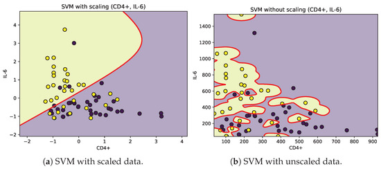
Figure 5.
Decision boundaries (red) for SVM classification of moderate (purple) and severe (yellow) patients according to CD4+ and IL-6.
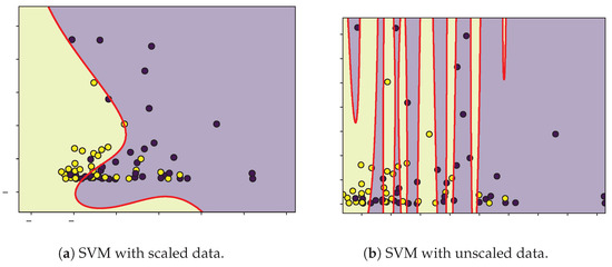
Figure 6.
Decision boundaries (red) for SVM classification of moderate (purple) and severe (yellow) patients according to CD4+ and TRPV-1.
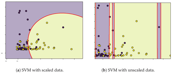
Figure 7.
Decision boundaries (red) for SVM classification of moderate (purple) and severe (yellow) patients according to TRPV-1 and IL-6.
The SVM analysis identified IL-6, TRPV-1, and CD as relevant variables for classifying patients according to the severity of their symptoms. However, given the limited sample size, the decision boundaries were narrow, and the contributions of these features showed considerable overlap between moderate and severe groups. Biologically, IL-6 is a pro-inflammatory cytokine associated with cytokine storm and unfavorable COVID-19 outcomes [57], yet its temporal fluctuations and context-dependent expression may weaken its discriminative ability in small datasets. TRPV-1, a non-selective cation channel implicated in neuroimmune modulation and inflammatory process [58,59], displayed inconsistent separation patterns, suggesting its role may be secondary or influenced by comorbidities and medication. Similarly, CD T-cell counts, which often decrease in severe infections, exhibited large intra-group variability, reflecting transient immune exhaustion rather than a reliable biomarker of severity.
These findings suggest that within our dataset, IL-6, TRPV-1, and CD alone may not serve as robust predictors of disease severity when analyzed independently. The SVM decision surface likely reflects partial correlations among these biomarkers rather than distinct mechanistic pathways. Expanding the feature set to include systemic inflammation and tissue-damage markers such as C-reactive protein, ferritin, or viral load could strengthen model generalizability and biological interpretability.
From a modeling perspective, these patient-level results complement the epidemiological component by illustrating biological variability within the infection compartments. The moderate and severe SVM groups correspond approximately to compartments and in the epidemic model, while less symptomatic or asymptomatic cases correspond to and A (whose data were not taken into account due to their small numbers compared to the patients who reached the hospital). The overlap among SVM classes thus parallels the gradual rather than discrete transition of infection severity in the mechanistic model.
3.4.2. Parameter Estimation
Once the patients were classified according to their symptomatology, the model was adjusted by estimating the parameters using the accumulated data of patients with moderate or severe infections (Supplementary Material S2). The accumulated flows used in the fitting were not obtained simply by summing the model incidences, but rather by reconstructing them from the daily infection flows generated by the model (see Appendix B). In the bootstrap procedure, daily incidences of new moderate and severe cases were first simulated under a Poisson distribution with mean equal to the model-predicted flows, and then accumulated to obtain synthetic datasets consistent with the observational format. This approach ensures that the variability of daily counts is realistically incorporated, while the accumulated structure of the data is preserved. In addition, certain demographic and biological parameters were fixed according to values reported in the literature (e.g., natural mortality rate , recruitment , and latency period ), while the transmission rates, progression probabilities, and recovery/mortality rates were estimated.
To perform parameter estimation, the ranges of values stipulated in Table 1 were used, and the initial estimates used in the initial conditions and parameters are listed in Table 3. The natural mortality rate was fixed as , consistent with a mean life expectancy of 75 years [2]. The recruitment rate was defined as with a constant reference population size , following the demographic equilibrium approach commonly used in epidemiological models [2,14]. The latent-to-infectious rate was fixed at , corresponding to a mean latent period of 5 days, in line with estimates of incubation and viral shedding for SARS-CoV-2 [60,61]. The package used for data processing was “Pandas 2.0.3” and for parameter fitting “lmfit 1.3.3” [62] was used together with the “minimize” function and the selected optimization method was “lbfgsb” (L-BFGS-B). In this implementation, the objective function minimized by the optimizer corresponds to the L2-norm of the relative residuals between model predictions and observed data, together with a penalty term that enforces the biological constraint . Explicitly, the functional is given by
where represents the vector of parameters to be estimated (without vaccination or treatment ()), N is the number of data points, is the cumulative number of infected individuals in stage k (, for moderate and severe cases, respectively) predicted by the model at time for parameters ; denotes the corresponding cumulative number of observed cases at time , and is a small constant introduced to avoid division by zero and to reduce the dominance of large counts in the residuals. Meanwhile, represents the penalty function associated with the vector of probabilities , which allows us to disregard cases where the total probability of passing to a symptomatological stage is greater than one. Moreover, the penalty considered is given by

Table 3.
Parameter estimation and bootstrap confidence intervals for the model without vaccination or treatment.
Therefore, penalizes with times the excess over 1 if ; otherwise, there is no penalty. In expanded terms, can be written as to implement in the computational language used, considering the accumulated dates for the model and real cases. Thus, the first term in corresponds to the weighted least squares criterion (L2-norm of relative residuals), while the second term discards parameter combinations that are biologically infeasible by imposing a large quadratic penalty whenever the sum of transition probabilities exceeds one. The term prevents division by very small denominators and ensures numerical stability. In this study, we set , following a data-scaled normalization approach that balances the relative weighting of early and late observations. Alternative formulations, such as fixing or a small constant, were tested but resulted in less stable optimization when case counts varied by several orders of magnitude.
The results of the parameter estimation are listed in Table 3, and the population values were rounded. In addition, model fit plots for patients with moderate (Figure 8a) and severe symptoms (Figure 8b) are shown, in which we applied a parametric bootstrap on daily flows (Poisson noise, , seed = 12345) to obtain 95% CI for parameters and the bootstrap correlation matrix (Figure 9). The coefficients of determination () for moderately and severely infected patients were 0.9330 and 0.9471, respectively. Moreover, for the overall fit (considering both populations) the coefficients of Akaike and Bayesian information criteria were −1005.78595 and −958.662284, respectively.
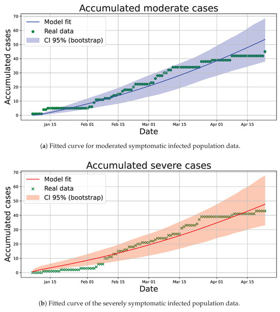
Figure 8.
Fitted curves and confidence intervals (CIs) to accumulated data for infected populations used to perform the parameter estimation.
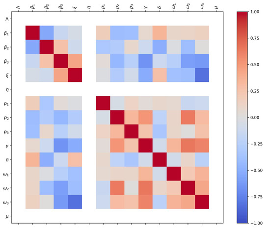
Figure 9.
Parameter correlation matrix obtained from the bootstrap analysis. The color bar on the right indicates the Pearson correlation coefficient ranging from (blue) to (red). White tones denote weak or absent correlations, often corresponding to fixed parameters during estimation.
Parameter estimation was performed with the accumulated data instead of the daily data because the presence of many days where no new moderate or severe patients were admitted (zero values in the daily records) tends to fit an estimated curve decreasing asymptotically to zero, which does not reflect the existence of peaks of infected patients in the sampling time.
The parameter correlation matrix obtained from the bootstrap analysis (Figure 9) summarizes the pairwise relationships between estimated parameters. The color scale on the right represents the Pearson correlation coefficient, ranging from (strong negative correlation, blue) to (strong positive correlation, red). White or near-neutral tones correspond to weak or absent correlation, which in some cases reflects parameters that were fixed during estimation (e.g., , , or ). The upper-left block shows strong positive correlations among transmission parameters (, , ), suggesting that changes in one transmission pathway may be partially compensated by others. Similarly, moderate correlations appear between symptom-progression probabilities (, , ) and recovery or lethality rates (, ), indicating coupled effects between clinical severity and removal processes. These structured correlation patterns confirm that the model captures biologically consistent relationships among transmission, progression, and recovery parameters while maintaining overall identifiability.
3.4.3. Impact of Exogenous Factors
Once the parameters have been estimated, the subsequent analysis of the effect of treatment is exemplified individually on the severely infected (Figure 10), as they are of special interest because of the costs associated with their care and the risk of loss of life. Considering an initial ad hoc population composed of 100 000 susceptibles and one symptomatic infected of each type (mild, moderate and severe); the remaining epidemiological sub-populations were considered null.
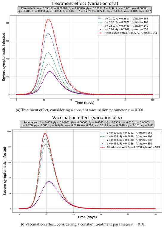
Figure 10.
Exogenous factor effect on severely symptomatic population dynamics . The population dynamics in red, considering the estimated parameters shown in the Table 3.
Figure 10a shows that increasing the rate of symptom reversal, that is, reducing the time in which the treatment affects the patient, allows us to decrease the maximum number of infections () appreciably. In our simulations, we used the range shown for from 0.10 to 0.70, which allowed decreases of 19.025% to 69.560% in , respectively. These reductions were estimated considering the without treatment and vaccination over the corresponding to the variational limits of ; for example, the reduction . Moreover, its effect over is not significant and tends to increase slightly (Figure 4a); therefore, it tends to decrease the peak of infected, but it does not reduce significantly over the disease-free scenario as shown in the Figure 10a.
In Figure 10b, we observed an increase in the vaccination rate, that is, increasing the vaccination speed in the range of , also allowed a slight decrease in the maximum number of infected () population without vaccination or treatment. In this case, we used a range for from 0.001 to 0.05, which caused a decrease from 0.822% to 63.962%, as well as a unique case in which the vaccination had a great impact over the infected peak when we assumed the maximum value ( = 0.05)—comparable with the maximum effect of the treatment. In contrast to the treatment scenario, the vaccination drastically reduces the , and it means that this strategy should be implemented as soon as possible when a outbreak is emerging in order to avoid endemic scenarios.
4. Discussion
The model assumes that asmptomatics can transmit the disease [3,24,63] and transmission rates follow the order , reflecting the assumptions that asymptomatic individuals () are less infectious than symptomatic individuals () due to lower viral load and less frequent coughing, while moderate () and severe () cases have limited mobility or are isolated. This aligns with studies indicating lower average transmission by asymptomatic individuals [3,25,50,60]. However, considering mobility alongside biological factors could alter the order to with , suggesting that high mobility among asymptomatic individuals increases their contact frequency with susceptible populations, resulting in a greater net transmissibility than mildly symptomatic individuals [27,63,64]; meanwhile, the order between moderate and severe cases is maintained due to isolation, zero mobility, and care by protected health personnel, minimizing their transmission. It is corroborated by our parameter estimation results, we found that ; however, , where this relation could have been due to the lack of data on mild symptomatic cases, although if later confirmed with data from such cases, it could be justified as a consequence of the high viral load in moderately and severely infected patients compared to mild ones, in addition to the social movement restriction measures implemented in Peru at that time, and also because the data collection was carried out in a hospital that mostly treated patients with more severe conditions.
The sensitivity results for (Figure 4a) indicate that decreasing the inflow and/or transmission rates () and increasing the vaccination and/or recovery rate allow us to decrease and control the development of an epidemic.
From the results in Table 2, we can state that the unscaled classification model exhibits better performance and fit than the model with scaled data. Because the optimized parameter C in the unscaled model is lower than that in the scaled model, overfitting can be avoided by having a wider separation margin and greater tolerance to misclassifications, while the lower values are close to zero in the case of the unscaled model with respect to the scaled model. It can be interpreted that in this case, the model behaves as a quasilinear separator. The positive and negative true values indicate that the unscaled model is the best qualifier. We consider that because of the limited data and because the data do not show an unambiguous separation in each class, it is not possible to generalize the application of the optimized unscaled model to any group of patients to be classified.
From an epidemiological standpoint, the SVM-based classification contributes to understanding the heterogeneity of infection within the modeled population. Patients classified as “severe” correspond to higher-risk compartments within the epidemic model (e.g., and ), whereas moderate or asymptomatic individuals relate to and A. The limited separability of IL-6, TRPV-1, and CD profiles supports the notion that biological variability within these compartments is high, particularly during early epidemic phases when host response markers fluctuate and sample sizes remain small.
While IL-6 has been consistently reported as a marker of inflammation and severe COVID-19 outcomes [57,65], our results highlight that its discriminatory capacity may depend on the timing of measurement and co-expression of immune mediators. TRPV-1 expression may modulate inflammatory signaling but appears context-dependent, potentially varying with comorbid conditions or pharmacological treatment [58,59]. CD depletion, a hallmark of immune dysfunction, also displayed variability that may reflect transient immune exhaustion rather than irreversible damage.
The observed overlap in biomarker-based classification reinforces the idea that biological processes underlying COVID-19 severity exist on a continuum rather than in distinct categories. IL-6 elevation, CD depletion, and TRPV-1 signaling interact through inflammatory and immune feedback loops, which may fluctuate during disease progression. Therefore, while SVMs can detect these multidimensional patterns, their predictive value is constrained by sample size and the timing of biomarker measurement. Future studies combining longitudinal immune profiling and epidemic modeling could help disentangle these intertwined mechanisms and clarify how host-level responses shape transmission dynamics at the population scale.
These observations underscore the complexity of linking individual-level biomarkers to population-level epidemic outcomes. By integrating both modeling layers, our framework illustrates how mechanistic epidemiological parameters and clinical biomarkers jointly inform disease progression and population health dynamics.
In the parameter estimation process, the residuals were normalized using a constant equal to the mean of the observed data. This adaptive normalization helped prevent the optimization from being dominated by large cumulative values and reduced sensitivity to noise in the early stages of the epidemic curve. Choosing mean(data) effectively scales the fitting process to the overall magnitude of the outbreak, leading to more robust and interpretable estimates. In contrast, a fixed constant such as would have imposed equal weighting across all time points, potentially underrepresenting early fluctuations or overemphasizing late dynamics.
We note that the model estimated a relatively high number of asymptomatic agents. This finding reflects uncertainties in the initial estimates of infected individuals, especially under limited testing capacity during outbreak phases. Similar results have been reported in the literature [64]. From the results obtained in Table 3, it is observed that the probability of being asymptomatic (P = 0.8642) is high with respect to developing any type of symptom, which has been corroborated both for cases of COVID-19 and for cases of respiratory syncytial virus infection. In the case of COVID-19, estimates have been reported in small samples of hospital populations of 41.8% of asymptomatic patients, with a higher frequency of these cases in the age range of 20–29 years and predominantly in the female sex [66]; another study also reported the presence of 40.7% of asymptomatic patients with a higher predominance in young people with an average age of 37.2 years but without a significant difference between sexes [67]. In the specific case of Peru, there are reports of a prevalence of 56% of asymptomatic patients in the general population in the city of Lima [68]. Worldwide, the existence of reported cases of asymptomatic cases for COVID-19 varies from 4% to more than ∼80% [69,70,71].
Similarly, in the case of respiratory syncytial virus (RSV) infection, the frequency of asymptomatic infected patients has been reported to be between ∼25% and 80% [72] and in cases of influenza with percentages higher than ∼50% [73]. These results reflect a myriad of results due to population heterogeneity and immunological and genetic characteristics of human populations; however, it makes the high frequencies of asymptomatic patients feasible, similar to those estimated in our case.
Recent studies have emphasized that large estimated proportions of asymptomatic individuals often arise from a combination of epidemiological and methodological factors rather than purely biological ones. In particular, Albi et al. [74] demonstrated through a multiscale modeling framework that under conditions of limited testing and delayed symptom onset, the apparent prevalence of asymptomatic cases can be significantly overestimated due to observational bias and structural identifiability issues. These biases tend to be most pronounced during early epidemic phases, when diagnostic coverage is low and detection probabilities differ between symptomatic and asymptomatic infections.
Meta-analyses have reported wide variability in the true proportion of asymptomatic SARS-CoV-2 infections, ranging from 17% to 81% across populations and study designs [75,76]. Such heterogeneity stems from differences in testing frequency, population age structure, viral variants, and immune history [77]. Consequently, our estimated value (P = 0.8642) should not be interpreted as a precise prevalence but rather as an emergent property of the model calibration given limited and hospital-centered data. This reinforces the importance of integrating seroprevalence surveys and systematic testing data in future parameter estimations to improve identifiability and avoid conflating unobserved infections with true asymptomatic proportions.
In Figure 8a,b, we observe that there is an acceptable fit between the data collected on the cumulative incidence of patients in the study period and the fit curve with the estimated parameters, which is reflected by the values of the metrics mentioned above, it is also pertinent to mention that the constant cumulative collected values are due to the fact that in the daily data collection no new severe or moderate patients were recorded on those days (Supplementary Material S2).
The correlation structure between parameters highlights the interdependence of epidemiological processes within the model. The positive association between parameters reflects that transmission rates are not independently identifiable when infection compartments overlap in their epidemiological roles, a phenomenon typical of multistage infectious models [78]. Meanwhile, moderate correlations between progression () and removal (, ) parameters suggest that the observed dynamics can be equally well explained by compensatory changes in disease severity or recovery rates—an issue also reported in sensitivity analyses of compartmental COVID-19 models [14,60]. The weak or null correlations observed for fixed parameters indicate stability of the estimation framework, reinforcing the robustness of the bootstrap approach in capturing uncertainty structure while avoiding overparameterization.
Increasing vaccination rates decreases the peak number of infected individuals and slightly delays infection onset (Figure 10b). Conversely, antiviral or pharmacological cough therapy that reduces symptom severity significantly decreases the peak number of infected individuals and advances the onset of the peak (Figure 10a). While the impact of the treatment on infection dynamics is appreciable on the population, it slightly increases , whereas vaccination dramatically decreases it. Considering these results, and the sensitivity to changes in transmission rates (Figure 3a), effective strategies could combine transmission containment measures like isolation or quarantine with slightly faster vaccination and early treatment.
A limitation of this study is the relatively small and homogeneous dataset used for SVM classification. This restricts the generalizability of the patient-level predictions and may underrepresent population heterogeneity. To partially mitigate this, we conducted an exploratory feature-importance analysis of the SVM, which revealed distinctive variables influencing classification performance. These findings provide interpretable insights despite the sample size constraint, and highlight avenues for improvement with larger and more diverse datasets.
This exploratory evaluation does not overcome the sample-size constraint but rather offers an interpretable framework for identifying candidate biomarkers whose discriminative capacity can be validated in larger, more heterogeneous populations.
We expanded the discussion to highlight the novelty of combining epidemic modeling and patient-level classification. This integration provides both a macroscopic and microscopic view of the pandemic. The epidemic model informs understanding of the transmission dynamics, while the SVM contributes to identifying high-risk patients. This dual perspective, supported by references [29,30,36], offers a more comprehensive framework that may be extended to other infectious diseases.
For future studies, a more in-depth qualitative study of the proposed mathematical model is recommended, examining the stability of the solutions. It is also advisable to increase the number of characteristics considered in the classification model, as well as to evaluate its applicability to other populations and/or acute respiratory diseases such as influenza. In parameter estimation, the population of deaths from the disease could be used to increase the accuracy of the values found, provided the database used is well-built. In addition, some limitations of the model should be addressed, such as considering multilinear incidence rates, considering similar recovery rates, not considering isolation or quarantine, and not considering the loss of immunity.
5. Conclusions
The mathematical model developed in this study integrates symptom-based stratification of infected individuals and the effects of exogenous interventions such as vaccination and treatment. The system exhibits both a disease-free equilibrium for and an endemic equilibrium for , consistent with classical epidemic thresholds. Sensitivity analyses and dynamic simulations showed that increasing the vaccination rate effectively reduces the basic reproduction number and can drive the system toward disease elimination. Conversely, enhancing the symptom reversion rate (representing faster treatment efficacy) mainly mitigates the infection peak without substantially reducing , suggesting that treatment acts as a stabilizing but not eradicating mechanism. These results emphasize that vaccination remains the most influential parameter in modulating the long-term epidemiological dynamics.
The bootstrap analysis of parameter estimation confirmed model identifiability and revealed biologically consistent correlations among transmission, progression, and recovery parameters. Strong associations between transmission coefficients indicate compensatory mechanisms among infectious stages, while moderate correlations between severity progression and removal rates highlight coupled clinical and epidemiological effects. This structure validates the internal coherence of the model and supports the robustness of the fitted parameter set.
In parallel, the integration of a Support Vector Machine (SVM) classifier with the mechanistic model provided complementary insights at the individual level. Using IL-6, TRPV-1, and CD markers without scaling improved classification performance, highlighting their discriminant power in differentiating moderate from severe infections. This dual modeling framework—linking population-level epidemic behavior with patient-level immunological profiles—offers a coherent and interpretable bridge between mechanistic and data-driven approaches. In the studied hospital population, vaccination strategies proved capable of shifting the system from an endemic to a disease-free state, while treatment strategies, although reducing the infection burden, are insufficient alone to suppress long-term transmission. Together, these findings provide quantitative guidance for optimizing intervention strategies in acute respiratory infections within similar epidemiological contexts.
Supplementary Materials
The following supporting information can be downloaded from https://www.mdpi.com/article/10.3390/covid5110190/s1, Table S1: Patient classification and biomarkers using to develop Support Vector Machines; Table S2: Time series data of moderate and severe patients using in the parameter estimation.
Author Contributions
Conceptualization, P.I.P.-G., E.C.-M., E.H.C.-V., L.A.-G. and R.L.-C.; methodology, P.I.P.-G., E.C.-M., E.H.C.-V., L.A.-G. and R.L.-C.; software, P.I.P.-G. and R.L.-C.; validation, P.I.P.-G., E.C.-M., D.T.G., G.T.P., E.C.C., C.L.Q. and R.L.-C.; formal analysis, P.I.P.-G. and R.L.-C.; investigation, P.I.P.-G., E.H.C.-V., L.A.-G., D.T.G., G.T.P., E.C.C., C.L.Q., E.E.A.-S. and E.R.-R.; resources, E.H.C.-V.; data curation, P.I.P.-G., E.C.-M., D.T.G., G.T.P., E.C.C. and C.L.Q.; writing—original draft preparation, P.I.P.-G. and R.L.-C.; writing—review and editing, P.I.P.-G., E.C.-M., E.H.C.-V., L.A.-G., D.T.G., G.T.P., E.C.C., C.L.Q., E.E.A.-S., E.R.-R. and R.L.-C.; visualization, P.I.P.-G., E.C.-M. and R.L.-C.; supervision, P.I.P.-G., E.C.-M., E.H.C.-V., L.A.-G., D.T.G., E.C.C., C.L.Q., E.E.A.-S., E.R.-R. and R.L.-C.; project administration, E.H.C.-V.; funding acquisition, E.H.C.-V. All authors have read and agreed to the published version of the manuscript.
Funding
This research was supported by Universidad Nacional Mayor de San Marcos—R.R. N° 016238-2020-R/UNMSM and project number B2010002m—PMULTIS 2020.
Institutional Review Board Statement
The study was conducted in accordance with the Declaration of Helsinki, and approved by Ethics Committee of Specific Studies for COVID-19 of the Social Health Security—ESSALUD (Code EI00001623, 12/22/2020).
Informed Consent Statement
Informed consent was obtained from all subjects involved in the study. Written informed consent has been obtained from the patient(s) to publish this paper.
Data Availability Statement
The original contributions about patient classification by symptoms severity presented in this study are included in Supplementary Materials Tables S1 and S2.
Acknowledgments
The authors thank the Universidad Nacional Mayor de San Marcos for funding this study. This research is part of the project “Study of the neuroimmune relationship in COVID-19 by identifying proinflammatory cytokines and neuropeptides released by TRPV1 activation. Bases for a proposal in the treatment of moderate and severe cases of the disease, funded by the Multidisciplinary Research Programme for research groups in COVID-19 (code B2010002m) and with the support of the Molecular Biology Unit of the HNGAI for the development of the experimental part.
Conflicts of Interest
The authors declare no conflicts of interest.
Abbreviations
The following abbreviations are used in this manuscript:
| SVMs | Support vector machines |
| IL-6 | Interleukin-6 |
| TRPV-1 | Transient Receptor Potential Vanilloid 1 |
| CD4+ | Helper T cells or T4 lymphocytes |
Appendix A. Reduced System of Ordinary Differential Equations and the Next-Generation Matrix
Appendix A.1. Proposed Reduced Mathematical Model
Appendix A.2. Derivation of the Basic Reproduction Number
First, the disease-free equilibrium point for the system (A1). In the disease-free equilibrium, the following condition must be met:
Replacing this condition in the system in equilibrium, we obtain:
After that, the calculations were performed using a next generation matrix. This methodology allows for the direct evaluation of the subsystem of the infected compartments:
The transition matrices between infected and uninfected states are defined as:
- : Matrix representing the flow of new infections in infected compartments. Epidemiologically, it represents the flow by direct or contact transmission of the disease.
- : Matrix formed by the transfer of individuals to infected compartments for reasons other than infection.
- : Matrix formed by outflows from infected compartments for reasons other than infection (infected outflow matrix).
- : Represents the net flow of the various infected compartments related to disease progression (transitions between infected compartments due to symptom progression and recovery, etc.), demographic phenomena (births, natural or disease-related death, migration, etc.), and exogenous factors (such as vaccination and treatment).
From the system (A3), the column vector for the occurrence of new infections and the transfer matrix are formed. In the present case, they take the following forms:
We proceed to calculate the Jacobian of the matrices and , evaluating (A4) and (A5) at the disease-free equilibrium point (A2).
We proceeded to calculate the inverse matrix of V (A7) and using (A6); subsequently, we determined the matrix product , which is called the next generation matrix. Following this estimation methodology, the basic reproductive number for an epidemic outbreak is defined as the spectral radius of the next-generation matrix [41,42]:
By performing the relevant algebraic simplifications, the following basic reproductive number is obtained:
where
Appendix B. Theoretical Formulation of the Cost Functional
In this section, we provide a mathematical description of the cost functional used in the parameter estimation procedure. Let denote the cumulative number of infected individuals in class (moderate and severe cases, respectively) predicted by the model with parameter vector , and let represent the corresponding observed data at discrete times , .
The cumulative infection flows for each class are defined as
where denotes the transition rate from the latent compartment L to the infectious compartment . These integrals capture the total number of individuals that have progressed into the respective symptomatic states up to time t.
To estimate parameters, we minimize the discrepancy between model predictions and observed data using a weighted least-squares criterion. The standard (absolute) norm of residuals is defined as
which measures the total squared deviation between model outputs and observations. However, this absolute formulation can overemphasize classes or time points with large case counts, especially when data are unbalanced.
To overcome this, we employ the relative -norm, normalizing each residual by its corresponding observed value plus a small positive constant , yielding
where is a penalty function enforcing the biological constraint . This relative normalization ensures that each data point contributes proportionally to the objective function, regardless of scale or magnitude, and enhances numerical stability when fitting to cumulative epidemic data spanning several orders of magnitude.
From a functional-analytic perspective, defines a weighted least-squares problem over the data space endowed with the inner product
Minimizing thus corresponds to finding the projection of model outputs onto the data space under this weighted inner product, balancing the influence of each infected class. The inclusion of prevents division by zero and improves conditioning of the optimization problem, following the regularization principles described in [79,80].
This formulation is consistent with data-scaling practices in inverse problems and epidemiological model fitting [81,82]. The resulting cost functional achieves a compromise between absolute and relative error minimization, ensuring robust parameter estimation even when the observed data are heterogeneous or sparse. A graphical summary is showed in the following scheme (Figure A1):
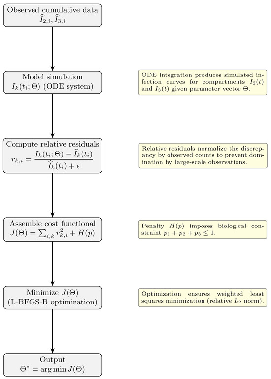
Figure A1.
Flowchart of the parameter estimation methodology. In the output, represents the vector of optimal parameters estimated by the methodology presented.
Appendix C. Probability Distributions for the PRCC Results
All uniformly distributed parameters were sampled within biologically and epidemiologically plausible ranges derived from Table 1. Normal sampling was used when prior estimates from the literature provided a central mean value and associated variability, following the Latin Hypercube approach implemented in the PRCC analysis. For , the mean and standard deviation (mean = 0.16975, sd = 0.14275) were chosen to reflect reported heterogeneity in recovery rates across COVID-19 cohorts [60,64,70]. Similarly, and were drawn from normal distributions emphasizing their expected central tendency (0.5 and 0.4, respectively) with moderate dispersion to capture behavioral and biological variability. This mixed sampling scheme (Uniform and Normal) ensures adequate exploration of the parameter space while preserving biological interpretability. A graphical summary of the PRCC workflow is showed in the following scheme (Figure A2):
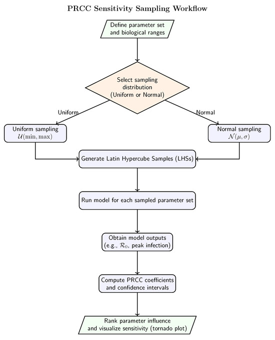
Figure A2.
Schematic representation of the PRCC sensitivity analysis procedure, illustrating the generation of parameter samples using Uniform or Normal distributions, model evaluation for each parameter set, and subsequent computation of partial rank correlation coefficients.

Table A1.
Sampling distributions and baseline values used for the PRCC (Partial Rank Correlation Coefficient) sensitivity analysis. Parameters with Normal distributions were sampled using truncated normal laws to ensure biological plausibility.
Table A1.
Sampling distributions and baseline values used for the PRCC (Partial Rank Correlation Coefficient) sensitivity analysis. Parameters with Normal distributions were sampled using truncated normal laws to ensure biological plausibility.
| Parameter | Distribution Type | Lower Bound | Upper Bound | Parameters (mean, sd) |
|---|---|---|---|---|
| Uniform | — | |||
| Uniform | — | |||
| Uniform | — | |||
| Uniform | — | |||
| Uniform | 10 | — | ||
| Uniform | — | |||
| Uniform | — | |||
| Uniform | — | |||
| Uniform | — | |||
| Uniform | — | |||
| Uniform | — | |||
| Uniform | — | |||
| Uniform | — | |||
| Uniform | — | |||
| Normal | 0 | 1 | mean = , sd = | |
| Normal | 0 | 1 | mean = , sd = | |
| Normal | 0 | 1 | mean = , sd = |
References
- Kermack, W.O.; McKendrick, A.G. A contribution to the mathematical theory of epidemics. Proc. R. Soc. Lond. Ser. A Contain. Pap. A Math. Phys. Character 1927, 115, 700–721. [Google Scholar]
- Anderson, R.M.; May, R.M. Infectious Diseases of Humans: Dynamics and Control; Oxford University Press: Oxford, UK, 1992. [Google Scholar]
- Arino, J.; Portet, S. A simple model for COVID-19. Infect. Dis. Model. 2020, 5, 309–315. [Google Scholar] [CrossRef]
- Ledder, G. Incorporating mass vaccination into compartment models for infectious diseases. Math. Biosci. Eng. 2022, 19, 9457–9480. [Google Scholar] [CrossRef] [PubMed]
- Antonelli, E.; Piccolomini, E.L.; Zama, F. Switched forced SEIRDV compartmental models to monitor COVID-19 spread and immunization in Italy. Infect. Dis. Model. 2022, 7, 1–15. [Google Scholar] [CrossRef]
- Hou, Y.; Bidkhori, H. Multi-feature SEIR model for epidemic analysis and vaccine prioritization. PLoS ONE 2024, 19, e0298932. [Google Scholar] [CrossRef] [PubMed]
- Li, R.; Song, Y.; Qu, H.; Li, M.; Jiang, G.P. A data-driven epidemic model with human mobility and vaccination protection for COVID-19 prediction. J. Biomed. Inform. 2024, 149, 104571. [Google Scholar] [CrossRef] [PubMed]
- Kiselev, I.N.; Akberdin, I.R.; Kolpakov, F.A. Delay-differential SEIR modeling for improved modelling of infection dynamics. Sci. Rep. 2023, 13, 13439. [Google Scholar] [CrossRef]
- Lacy, A.; Igoe, M.; Das, P.; Farthing, T.; Lloyd, A.L.; Lanzas, C.; Odoi, A.; Lenhart, S. Modeling impact of vaccination on COVID-19 dynamics in St. Louis. J. Biol. Dyn. 2023, 17, 2287084. [Google Scholar] [CrossRef]
- Han, X.; Liu, H.; Lin, X.; Wei, Y.; Ming, M. Dynamic analysis of a VSEIR model with vaccination efficacy and immune decline. Adv. Math. Phys. 2022, 2022, 7596164. [Google Scholar] [CrossRef]
- Pathak, S.; Kota, V.R. An influential study of a time-delayed epidemic model incorporating vaccination and treatment interventions. Adv. Contin. Discret. Models 2025, 2025, 57. [Google Scholar] [CrossRef]
- Zephaniah, O.C.; Nwaugonma, U.I.R.; Chioma, I.S.; Adrew, O. A mathematical model and analysis of an SVEIR model for streptococcus pneumonia with saturated incidence force of infection. Math. Model. Appl. 2020, 5, 16–38. [Google Scholar] [CrossRef]
- Chen, T.M.; Rui, J.; Wang, Q.P.; Zhao, Z.Y.; Cui, J.A.; Yin, L. A mathematical model for simulating the phase-based transmissibility of a novel coronavirus. Infect. Dis. Poverty 2020, 9, 24. [Google Scholar] [CrossRef] [PubMed]
- Ferguson, N.M.; Cummings, D.A.; Fraser, C.; Cajka, J.C.; Cooley, P.C.; Burke, D.S. Strategies for mitigating an influenza pandemic. Nature 2006, 442, 448–452. [Google Scholar] [CrossRef] [PubMed]
- Boianelli, A.; Nguyen, V.K.; Ebensen, T.; Schulze, K.; Wilk, E.; Sharma, N.; Stegemann-Koniszewski, S.; Bruder, D.; Toapanta, F.R.; Guzmán, C.A.; et al. Modeling influenza virus infection: A roadmap for influenza research. Viruses 2015, 7, 5274–5304. [Google Scholar] [CrossRef]
- Hernandez-Vargas, E.A.; Velasco-Hernandez, J.X. In-host modelling of COVID-19 kinetics in humans. medRxiv 2020, 20044487. [Google Scholar] [CrossRef]
- Smith, A.M. Host-pathogen kinetics during influenza infection and coinfection: Insights from predictive modeling. Immunol. Rev. 2018, 285, 97–112. [Google Scholar] [CrossRef]
- Della Marca, R.; Loy, N.; Tosin, A. An SIR model with viral load–dependent transmission. J. Math. Biol. 2023, 86, 61. [Google Scholar] [CrossRef]
- Dimarco, G.; Perthame, B.; Toscani, G.; Zanella, M. Kinetic models for epidemic dynamics with social heterogeneity. J. Math. Biol. 2021, 83, 4. [Google Scholar] [CrossRef]
- Dimarco, G.; Toscani, G.; Zanella, M. Optimal control of epidemic spreading in the presence of social heterogeneity. Philos. Trans. R. Soc. A 2022, 380, 20210160. [Google Scholar] [CrossRef]
- Almocera, A.E.S.; Nguyen, V.K.; Hernandez-Vargas, E.A. Multiscale model within-host and between-host for viral infectious diseases. J. Math. Biol. 2018, 77, 1035–1057. [Google Scholar] [CrossRef]
- Bondesan, A.; Piralla, A.; Ballante, E.; Pitrolo, A.M.G.; Figini, S.; Baldanti, F.; Zanella, M. Predictability of viral load dynamics in the early phases of SARS-CoV-2 through a model-based approach. Math. Biosci. Eng. 2025, 22, 725–743. [Google Scholar] [CrossRef]
- DeVincenzo, J.P.; Wilkinson, T.; Vaishnaw, A.; Cehelsky, J.; Meyers, R.; Nochur, S.; Harrison, L.; Meeking, P.; Mann, A.; Moane, E.; et al. Viral load drives disease in humans experimentally infected with respiratory syncytial virus. Am. J. Respir. Crit. Care Med. 2010, 182, 1305–1314. [Google Scholar] [CrossRef] [PubMed]
- Rasmussen, A.L.; Popescu, S.V. SARS-CoV-2 transmission without symptoms. Science 2021, 371, 1206–1207. [Google Scholar] [CrossRef]
- Johansson, M.A.; Quandelacy, T.M.; Kada, S.; Prasad, P.V.; Steele, M.; Brooks, J.T.; Slayton, R.B.; Biggerstaff, M.; Butler, J.C. SARS-CoV-2 transmission from people without COVID-19 symptoms. JAMA Netw. Open 2021, 4, e2035057. [Google Scholar] [CrossRef]
- Ip, D.K.; Lau, L.L.; Leung, N.H.; Fang, V.J.; Chan, K.H.; Chu, D.K.; Leung, G.M.; Peiris, J.M.; Uyeki, T.M.; Cowling, B.J. Viral shedding and transmission potential of asymptomatic and paucisymptomatic influenza virus infections in the community. Clin. Infect. Dis. 2017, 64, 736–742. [Google Scholar] [CrossRef]
- Gandhi, M.; Yokoe, D.S.; Havlir, D.V. Asymptomatic transmission, the Achilles’ heel of current strategies to control COVID-19. N. Engl. J. Med. 2020, 382, 2158–2160. [Google Scholar] [CrossRef] [PubMed]
- D’Agostino McGowan, L.; Grantz, K.H.; Murray, E. Quantifying uncertainty in infectious disease mechanistic models. Am. J. Epidemiol. 2021. [Google Scholar] [CrossRef] [PubMed]
- Dat, T.T.; Protin, F.; Nguyen, T.T.H.; Martel, J.; Nguyen, D.T.; Piffault, C.; Rodríguez, W.; Figueroa, S.; Lê, H.V.; Tuschmann, W.; et al. Epidemic Dynamics via Wavelet Theory and Machine Learning with Applications to COVID-19. Biology 2020, 9, 477. [Google Scholar] [CrossRef]
- Cheng, Y.Y.; Cheng, R.; Xu, T.; Tan, X.; Bai, Y. Machine Learning Techniques Applied to COVID-19 Prediction: A Systematic Literature Review. Bioengineering 2025, 12, 514. [Google Scholar] [CrossRef]
- Cortes, C.; Vapnik, V. Support-vector networks. Mach. Learn. 1995, 20, 273–297. [Google Scholar] [CrossRef]
- Noble, W.S. What is a support vector machine? Nat. Biotechnol. 2006, 24, 1565–1567. [Google Scholar] [CrossRef]
- Byvatov, E.; Schneider, G. Support vector machine applications in bioinformatics. Appl. Bioinform. 2003, 2, 67–77. Available online: http://europepmc.org/abstract/MED/15130823 (accessed on 21 August 2025).
- Ben-Hur, A.; Ong, C.S.; Sonnenburg, S.; Schölkopf, B.; Rätsch, G. Support vector machines and kernels for computational biology. PLoS Comput. Biol. 2010, 6, e1000173. [Google Scholar] [CrossRef] [PubMed]
- Aktar, S.; Ahamad, M.M.; Rashed-Al-Mahfuz, M.; Azad, A.K.; Uddin, S.; Kamal, A.H.; Alyami, S.A.; Lin, P.I.; Islam, S.M.; Quinn, J.M.; et al. Machine Learning Approach to Predicting COVID-19 Disease Severity. JMIR Med. Inform. 2021, 4, e25884. [Google Scholar] [CrossRef] [PubMed]
- Santosh, K. AI-Driven Tools for Coronavirus Outbreak: Need of Active Learning and Cross-Population Train/Test Models on Multitudinal/Multimodal Data. J. Med. Syst. 2020, 44, 93. [Google Scholar] [CrossRef]
- Rivera-Tafur, E. Situación epidemiológica de las infecciones respiratorias agudas (IRA) en el Perú hasta la SE 06–2022. Bol. Epidemiol. 2022, 28, 374–377. [Google Scholar]
- Muñoz, C.M.M.; Basurto, V.A.D.; Anchundia, J.P.C.; Martinetti, G.G.H. Descripción y análisis de infecciones respiratorias agudas en niños menores de 5 años. Polo Del Conoc. 2021, 6, 1108–1123. [Google Scholar]
- MINSA. Resolución Ministerial-139-2020-Minsa: Documento Técnico—Prevención y Atención de Personas Afectadas por COVID-19 en el Perú; Documento Técnico; MINSA: Lima, Peru, 2020. [Google Scholar]
- Hethcote, H.W. The mathematics of infectious diseases. SIAM Rev. 2000, 42, 599–653. [Google Scholar] [CrossRef]
- Diekmann, O.; Heesterbeek, J.; Roberts, M.G. The construction of next-generation matrices for compartmental epidemic models. J. R. Soc. Interface 2010, 7, 873–885. [Google Scholar] [CrossRef]
- Van den Driessche, P.; Watmough, J. Reproduction numbers and sub-threshold endemic equilibria for compartmental models of disease transmission. Math. Biosci. 2002, 180, 29–48. [Google Scholar] [CrossRef]
- Harko, T.; Lobo, F.S.; Mak, M.K. Exact analytical solutions of the Susceptible-Infected-Recovered (SIR) epidemic model and of the SIR model with equal death and birth rates. Appl. Math. Comput. 2014, 236, 184–194. [Google Scholar] [CrossRef]
- Schlickeiser, R.; Kröger, M. Analytical modeling of the temporal evolution of epidemics outbreaks accounting for vaccinations. Physics 2021, 3, 386–426. [Google Scholar] [CrossRef]
- Schlickeiser, R.; Kröger, M. Analytical Solution of the Susceptible-Infected-Recovered/Removed Model for the Not-Too-Late Temporal Evolution of Epidemics for General Time-Dependent Recovery and Infection Rates. Covid 2023, 3, 1781–1796. [Google Scholar] [CrossRef]
- Cilloniz, C.; Luna, C.M.; Hurtado, J.C.; Marcos, M.Á.; Torres, A. Respiratory viruses: Their importance and lessons learned from COVID-19. Eur. Respir. Rev. 2022, 31, 220051. [Google Scholar] [CrossRef]
- Xin, H.; Li, Y.; Wu, P.; Li, Z.; Lau, E.H.; Qin, Y.; Wang, L.; Cowling, B.J.; Tsang, T.K.; Li, Z. Estimating the latent period of coronavirus disease 2019 (COVID-19). Clin. Infect. Dis. 2022, 74, 1678–1681. [Google Scholar] [CrossRef] [PubMed]
- Abrams, S.; Wambua, J.; Santermans, E.; Willem, L.; Kuylen, E.; Coletti, P.; Libin, P.; Faes, C.; Petrof, O.; Herzog, S.A.; et al. Modelling the early phase of the Belgian COVID-19 epidemic using a stochastic compartmental model and studying its implied future trajectories. Epidemics 2021, 35, 100449. [Google Scholar] [CrossRef]
- Aguilar, J.B.; Faust, J.S.; Westafer, L.M.; Gutierrez, J.B. Modeling the Impact of Asymptomatic Carriers on COVID-19 Transmission Dynamics During Lockdown. medRxiv 2020. [Google Scholar] [CrossRef]
- Arino, J.; Brauer, F.; van den Driessche, P.; Watmough, J.; Wu, J. Simple models for containment of a pandemic. J. R. Soc. Interface 2006, 3, 453–457. [Google Scholar] [CrossRef]
- Aguirre-Siancas, E.E.; Colona-Vallejos, E.; Ruiz-Ramirez, E.; Becerra-Bravo, M.; Alzamora-Gonzales, L. Sustancia P, citocinas proinflamatorias, receptor de potencial transitorio vaniloide tipo 1 y COVID-19: Una hipótesis de trabajo. Neurología 2021, 36, 184. [Google Scholar] [CrossRef]
- McKinney, W. Data Structures for Statistical Computing in Python. In Proceedings of the 9th Python in Science Conference, Austin, TX, USA, 28 June–3 July 2010; Volume 445, pp. 56–61. [Google Scholar] [CrossRef]
- Pedregosa, F.; Varoquaux, G.; Gramfort, A.; Michel, V.; Thirion, B.; Grisel, O.; Blondel, M.; Prettenhofer, P.; Weiss, R.; Dubourg, V.; et al. Scikit-learn: Machine learning in Python. J. Mach. Learn. Res. 2011, 12, 2825–2830. [Google Scholar]
- Wilson, M. Support Vector Machines. In Encyclopedia of Ecology; Jørgensen, S.E., Fath, B.D., Eds.; Academic Press: Oxford, UK, 2008; pp. 3431–3437. [Google Scholar] [CrossRef]
- Adankon, M.M.; Cheriet, M. Support vector machine. In Encyclopedia of Biometrics; Springer: Berlin/Heidelberg, Germany, 2009; pp. 1303–1308. [Google Scholar]
- El Bouchefry, K.; de Souza, R.S. Learning in big data: Introduction to machine learning. In Knowledge Discovery in Big Data from Astronomy and Earth Observation; Elsevier: Amsterdam, The Netherlands, 2020; pp. 225–249. [Google Scholar]
- Del Valle, D.M.; Kim-Schulze, S.; Huang, H.H.; Beckmann, N.D.; Nirenberg, S.; Wang, B.; Lavin, Y.; Swartz, T.H.; Madduri, D.; Stock, A.; et al. An inflammatory cytokine signature predicts COVID-19 severity and survival. Nat. Med. 2020, 26, 1636–1643. [Google Scholar] [CrossRef]
- Silverman, H.A.; Chen, A.; Kravatz, N.L.; Chavan, S.S.; Chang, E.H. Involvement of neural transient receptor potential channels in peripheral inflammation. Front. Immunol. 2020, 11, 590261. [Google Scholar] [CrossRef]
- Munjuluri, S.; Wilkerson, D.A.; Sooch, G.; Chen, X.; White, F.A.; Obukhov, A.G. Capsaicin and TRPV1 channels in the cardiovascular and inflammatory response. Cells 2021, 11, 18. [Google Scholar] [CrossRef]
- He, X.; Lau, E.H.; Wu, P.; Deng, X.; Wang, J.; Hao, X.; Lau, Y.C.; Wong, J.Y.; Guan, Y.; Tan, X.; et al. Temporal dynamics in viral shedding and transmissibility of COVID-19. Nat. Med. 2020, 26, 672–675. [Google Scholar] [CrossRef] [PubMed]
- Lauer, S.A.; Grantz, K.H.; Bi, Q.; Jones, F.K.; Zheng, Q.; Meredith, H.; Azman, A.S.; Reich, N.G.; Lessler, J. The incubation period of coronavirus disease 2019 (COVID-19) from publicly reported confirmed cases: Estimation and application. Ann. Intern. Med. 2020, 172, 577–582. [Google Scholar] [CrossRef]
- Newville, M.; Stensitzki, T.; Allen, D.B.; Rawlik, M.; Ingargiola, A.; Nelson, A. LMFIT: Non-linear least-square minimization and curve-fitting for Python. Astrophys. Source Code Libr. 2016, ascl–1606. [Google Scholar]
- Byrne, A.W.; McEvoy, D.; Collins, A.B.; Hunt, K.; Casey, M.; Barber, A.; Butler, F.; Griffin, J.; Lane, E.A.; McAloon, C.; et al. Inferred duration of infectious period of SARS-CoV-2: Rapid scoping review and analysis of available evidence for asymptomatic and symptomatic COVID-19 cases. BMJ Open 2020, 10, e039856. [Google Scholar] [CrossRef] [PubMed]
- Li, R.; Pei, S.; Chen, B.; Song, Y.; Zhang, T.; Yang, W.; Shaman, J. Substantial undocumented infection facilitates the rapid dissemination of novel coronavirus (SARS-CoV-2). Science 2020, 368, 489–493. [Google Scholar] [CrossRef]
- Chen, T.; Wu, D.I.; Chen, H.; Yan, W.; Yang, D.; Chen, G.; Ma, K.; Xu, D.; Yu, H.; Wang, H.; et al. Clinical characteristics of 113 deceased patients with coronavirus disease 2019: Retrospective study. BMJ 2020, 368, m1091. [Google Scholar] [CrossRef] [PubMed]
- Ruiz Nápoles, J.B.; Ruiz Nápoles, K. Pacientes asintomáticos positivos a la COVID-19. Rev. Cuba. De Med. Mil. 2021, 50, 1. Available online: http://scielo.sld.cu/scielo.php?script=sci_arttext&pid=S0138-65572021000100011&nrm=iso (accessed on 29 October 2025).
- Ruiz Nápoles, J.B.; Ruiz Nápoles, K. Comparación de las características clínicas y epidemiológicas entre pacientes asintomáticos y sintomáticos con la COVID-19. Rev. Cuba. De Med. Mil. 2021, 50, 2. Available online: http://scielo.sld.cu/scielo.php?script=sci_arttext&pid=S0138-65572021000200007&nrm=iso (accessed on 29 October 2025).
- Reyes-Vega, M.F.; Soto-Cabezas, M.G.; Cárdenas, F.; Martel, K.S.; Valle, A.; Valverde, J.; Vidal-Anzardo, M.; Falcón, M.E.; Munayco, C.V. SARS-CoV-2 prevalence associated to low socioeconomic status and overcrowding in an LMIC megacity: A population-based seroepidemiological survey in Lima, Peru. EClinicalMedicine 2021, 34, 100801. [Google Scholar] [CrossRef] [PubMed]
- Petersen, I.; Phillips, A. Three quarters of people with SARS-CoV-2 infection are asymptomatic: Analysis of English household survey data. Clin. Epidemiol. 2020, 12, 1039–1043. [Google Scholar] [CrossRef]
- Byambasuren, O.; Cardona, M.; Bell, K.; Clark, J.; McLaws, M.L.; Glasziou, P. Estimating the extent of asymptomatic COVID-19 and its potential for community transmission: Systematic review and meta-analysis. Off. J. Assoc. Med. Microbiol. Infect. Dis. Can. 2020, 5, 223–234. [Google Scholar]
- Oran, D.P.; Topol, E.J. Prevalence of asymptomatic SARS-CoV-2 infection: A narrative review. Ann. Intern. Med. 2020, 173, 362–367. [Google Scholar] [CrossRef]
- Cohen, C.; Kleynhans, J.; Moyes, J.; McMorrow, M.L.; Treurnicht, F.K.; Hellferscee, O.; Wolter, N.; Martinson, N.A.; Kahn, K.; Lebina, L.; et al. Incidence and transmission of respiratory syncytial virus in urban and rural South Africa, 2017–2018. Nat. Commun. 2024, 15, 116. [Google Scholar] [CrossRef]
- Cohen, C.; Kleynhans, J.; Moyes, J.; McMorrow, M.L.; Treurnicht, F.K.; Hellferscee, O.; Mathunjwa, A.; von Gottberg, A.; Wolter, N.; Martinson, N.A.; et al. Asymptomatic transmission and high community burden of seasonal influenza in an urban and a rural community in South Africa, 2017–18 (PHIRST): A population cohort study. Lancet Glob. Health 2021, 9, e863–e874. [Google Scholar] [CrossRef]
- Albi, G.; Bongini, M.; Cristiani, E.; Kalise, D. Asymptomatic Transmission and Testing Limitations in Epidemic Outbreaks. J. Math. Biol. 2021, 83, 617–635. [Google Scholar] [CrossRef]
- Sah, P.; Fitzpatrick, M.C.; Zimmer, C.F.; Abdollahi, E.; Juden-Kelly, L.; Moghadas, S.M.; Singer, B.H.; Galvani, A.P. Asymptomatic SARS-CoV-2 infection: A systematic review and meta-analysis. Proc. Natl. Acad. Sci. USA 2021, 118, e2109229118. [Google Scholar] [CrossRef]
- Buitrago-García, D.; Egli-Gany, D.; Counotte, M.J.; Hossmann, S.; Imeri, H.; Ipekci, A.M.; Salanti, G.; Low, N. Occurrence and transmission potential of asymptomatic and presymptomatic SARS-CoV-2 infections: A living systematic review and meta-analysis. PLoS Med. 2020, 17, e1003346. [Google Scholar] [CrossRef] [PubMed]
- Boyton, R.J.; Altmann, D.M. The immunology of asymptomatic SARS-CoV-2 infection: What are the key questions? Nat. Rev. Immunol. 2021, 21, 762–768. [Google Scholar] [CrossRef] [PubMed]
- Champredon, D.; Dushoff, J.; Earn, D.J. Equivalence of the Erlang-distributed SEIR epidemic model and the renewal equation. SIAM J. Appl. Math. 2018, 78, 3258–3278. [Google Scholar] [CrossRef]
- Tikhonov, A.N.; Arsenin, V.Y. Solutions of Ill-Posed Problems; Wiley: New York, NY, USA, 1977. [Google Scholar]
- Hansen, P.C. Discrete Inverse Problems: Insight and Algorithms; SIAM: Philadelphia, PA, USA, 2010. [Google Scholar] [CrossRef]
- Banks, H.T.; Hu, S.; Thompson, W.C. Modeling and Inverse Problems in the Presence of Uncertainty; CRC Press: Boca Raton, FL, USA, 2014. [Google Scholar]
- Chowell, G. Fitting dynamic models to epidemic outbreaks with quantified uncertainty: A primer for parameter uncertainty, identifiability, and forecasts. Infect. Dis. Model. 2017, 2, 379–398. [Google Scholar] [CrossRef] [PubMed]
Disclaimer/Publisher’s Note: The statements, opinions and data contained in all publications are solely those of the individual author(s) and contributor(s) and not of MDPI and/or the editor(s). MDPI and/or the editor(s) disclaim responsibility for any injury to people or property resulting from any ideas, methods, instructions or products referred to in the content. |
© 2025 by the authors. Licensee MDPI, Basel, Switzerland. This article is an open access article distributed under the terms and conditions of the Creative Commons Attribution (CC BY) license (https://creativecommons.org/licenses/by/4.0/).